GIS Framework for Spatiotemporal Mapping of Urban Flooding

Abstract

This research aims to develop a framework using the Geographic Information System (GIS) to perform modeling and mapping of flood spatiotemporal variation in urban micro-watersheds. The GIS-framework includes a workflow of several methods and processes including delineation of urban watershed, generation of runoff hydrographs, and time series mapping of inundation depths and flood extent. This framework is tested in areas previously known to have experienced flooding at the University of Nevada, Las Vegas main campus, including Black Parking Lot (Blacklot) and East Mall. Calibration is performed by varying Digital Elevation Model (DEM) resolution, rainfall temporal resolution, and clogging factor whereas validation is performed using flood information from news reports and photographs. The testing at the Blacklot site resulted in calibration at 5 m DEM resolution and clogging factor of 0.83. The flood model resulted in an error of 24% between the estimated (26 inches/66 cm) and actual (34 inches/86.36 cm) flood depths. The estimated flood extents are consistent with the reported conditions and observed watermarks in the area. The flood beginning time estimated from the model is also consistent with the news reports. The testing at East Mall site also shows consistent results. The GIS framework provides spatiotemporal maps of flood inundation for visualization of flood dynamics. This research provides insight into flood modeling and mapping for a storm drain inlet-based watershed.

1. Introduction

Urban flooding is a complex phenomenon due to inhomogeneous nature of urban surfaces [1,2]. The intensity of urban flooding has increased throughout the world over the last few decades due to two main factors including urbanization (internal factor) and climate change (external factor) [3]. However, the effect of urbanization is more significant than climate change on local urban flooding [4]. Urban floods can occur due to a variety of reasons such as overtopping of flows in neighboring rivers and creeks, reservoir failure, and structural failure of drainage infrastructure. In general, urban flooding occurs when heavy rainfall is accompanied by limited capacity of drainage infrastructure. Urban floods can cause structural damages, environmental damages, affect the daily lives of people, and in extreme cases, can be fatal. The consequences of such damages can be high given that around 50% of the world’s population lives in urban areas ( 80% in United States) [5]. Therefore, it is of not a surprise that the authorities worldwide are investing in flood control and research to deal with this disastrous phenomenon.

Urban landscape is very dynamic and it therefore modulates the spatio-temporal behavior of flooding, further complicating its progression. Understanding urban flooding can help plan effective flood remediation measures and thus, a comprehensive approach should be developed to model flooding in urban watersheds. Generally, the process of developing a flood model is complex and time consuming. An urban flood model can either be simulated as a lumped model or a spatially distributed model. A distributed model requires more computational resources than a lumped model; however, it is considered to be more accurate than a lumped model to estimate floods in urban watersheds [6,7]. A large urban watershed can contain many micro-watersheds that individually, contribute stormwater to nearby drain inlets. Flooding in these micro-watersheds is typically affected by rainfall, drainage capacity of the inlet, land cover type, and surface depressions. Thus, these factors are conventionally used as input for flood modeling. These factors can be used for calibration, validation, and simulation of the flood models. To achieve accurate results, it is important to understand the impact of such factors on the hydrologic response of study sites [8].

An urban flood model, whether it is lumped or distributed, is an integration of hydrologic and hydraulic models. In case of urban flooding, hydrologic equations are used to produce runoff from rainfall whereas hydraulic equations are used to route the runoff. Hydraulic equations (e.g., Saint Venant equations) can either be implemented as one-dimensional (1D) or two-dimensional (2D) models. In case of flow in open channels and sewer system, 1D hydraulic equations provide reasonable approximation with less computational effort. However, in case of overland flow (sheet flow), 2D equations provide better approximation [9]. With the advancement of computational technology, 1D and 2D equations have also been combined as 1D/2D coupled numerical models to better predict the complex nature of flooding in urban watersheds [9,10,11]. Although flow routing in channels can be achieved using 1D models, overland sheet flow routing in urban watersheds can be challenging due to the existence of fixed obstacles (e.g., buildings) impacting the flow pattern. Buildings act as diversions of the flow path and inundation results vary based on the treatment of buildings in a model. Since there is no unique guideline on how to treat buildings, various researchers have adopted different strategies to include the impact of buildings in models such as Urban Inundation Model (UIM), 2D Cellular Automata (2D-CA) model, and Cellular Automata Dual-DraInagE Simulation (CADDIES) [12,13,14].

There are numerous established software applications (e.g., SWMM and MIKE-Urban) available for urban flood modeling [15]. Such applications have either a built-in Geographic Information System (GIS) data handler or they depend on an external GIS application for spatial data processing. GIS applications such as ArcGIS and QGIS provide the capability of integrating remote sensing information with GIS as well as ability to program workflow for spatially distributed modeling on a watershed scale. These applications have been used successfully in areas other than flooding including land use modeling [16]. These application provide the capabilities for both vector and raster data processing as well as Python scripting for model automation. In particular, being ubiquitous in academia, public, and private sector, ArcGIS is a convenient choice for urban flood modeling.

In this paper, we develop a GIS-based framework for flood modeling and mapping the spatiotemporal behavior of floods in urban micro-watersheds draining to storm drain inlets. This framework includes a workflow of several steps, programmed in ArcGIS computing environment, leading to spatio-temporal mapping and analysis of flooding in urban watersheds. The GIS-based framework couples the processes of watershed delineation, distributed flood modeling, visualization, and calibration and validation. To accomplish our research objective, a GIS framework is developed and tested to study flood events at two study sites at the University of Nevada, Las Vegas (UNLV) main campus.

This paper is organized as follows. Section 2 explains methods to develop the GIS-framework and Section 3 describes the study area and data used and highlights test results. Section 4 explains the test results at the study sites and Section 5 provides the conclusions of this research.

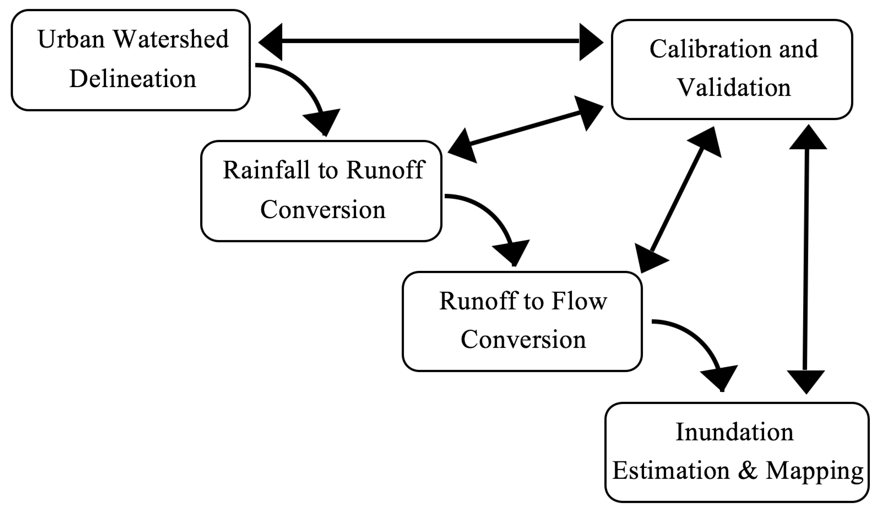
2. GIS Framework Development

This section describes the GIS-framework developed for modeling and mapping of flooding in urban micro-watersheds. The framework is divided into five components, namely: (i) urban watershed delineation; (ii) rainfall to runoff conversion; (iii) runoff to flow conversion; (iv) inundation estimation and mapping; and (v) calibration and validation as shown in Figure 1. The arrows show process flow where the calibration and validation can influence or be influenced by all other components. Watershed is delineated by constructing stream network for a point of interest (pour point), which can be a drain inlet or a low elevation point. Consequently, the inundation is mapped at this point of interest for a given rainfall event. In this framework, rainfall is first converted to runoff and subsequently to flow, which generates a runoff hydrograph at the pour point. In the case of a drain inlet, this runoff hydrograph is compared with the discharge hydrograph of the inlet to determine flooding characteristics. The flood depth is contoured over the elevation of the watershed surface to map flood extent. Finally, the calibration and validation of a flood model is performed by comparing the model output with observed data. The following subsections describe various components of the GIS framework.

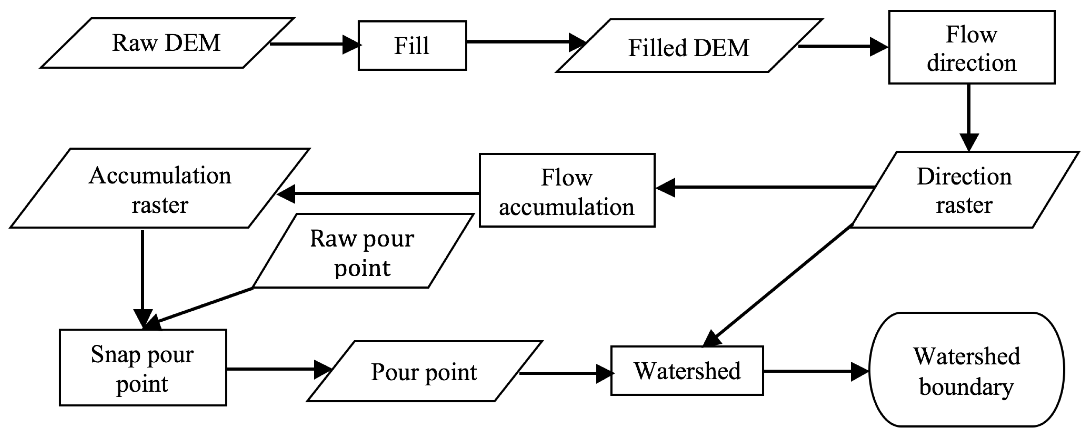
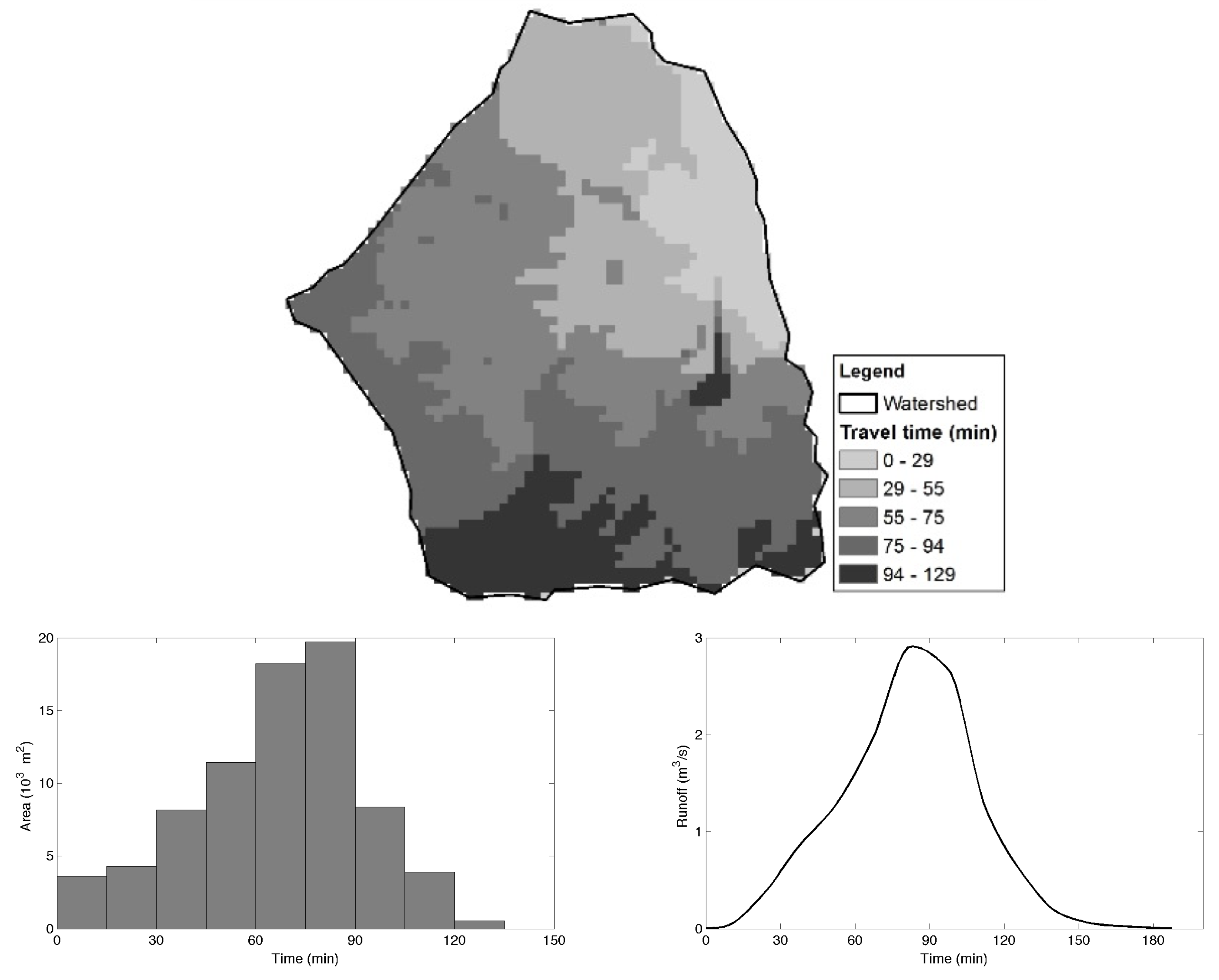
2.1. Urban Watershed Delineation

The watershed delineation component constructs a stream network using surface elevation. The streams that converge to the point of interest are used to delineate watershed boundary. This point of interest, which can be a depression or drain inlet, is considered to be the outlet point of the watershed. Typically, a Digital Terrain Model (DTM) is used to estimate flow directions, identify watershed divides, and flow concentration points. There are several ways to represent the terrain, such as in raster grid format that can be Digital Elevation Model (DEM), in vector format that can be Triangulated Irregular Network (TIN), as point cloud such as LiDAR data, and as isohypes called contours. Typically, point cloud and contours are converted to a DEM or TIN, and can be used for mapping landforms. Among the two, DEM is more convenient for distributed hydrologic models for its inherent advantage of raster processing. DEM can help find points of flow convergence (stream network) and divergence (watershed divide). Figure 2 shows a general process of delineating watershed in GIS adopted from Zhang et al. [17]. It illustrates a general process of building stream network and delineating watershed inside a GIS computing environment. It is noted that this process can be changed for specific needs, for example, the filtering and filling processes can be omitted if DEM has already been reconditioned by the data provider. The accumulation raster is typically thresholded to identify stream cells used to create a stream network. Moreover, DEM spatial resolution impacts the accuracy of stream network delineation and thus subsequent model output [18,19,20].

DEM data can have some inherent issues that need to be considered. Typically, it is reconditioned by removing elevation abnormalities, filling data gaps, and raising depressed pixels. Low-pass filtering is usually done to smooth the data, which in turn helps to remove abnormal peaks and flat areas, i.e., irregularities in elevation data [21]. The filling process results in depression removal by raising localized sink elevations to match the adjacent cell in order to ensure a continuous stream network. The reconditioned elevation data is further processed to estimate flow direction and accumulation in each cell. The cells exceeding a certain threshold of accumulation (typically 1% of maximum accumulation) are identified to form streams [22]. Often, threshold values can be based on the length of sheet flow (overland flow) in a watershed [22]. The flow accumulation greater than the threshold is considered to be stream network that is used to delineate watershed for a specific pour point. It is imperative that a given pour point is snapped to the stream network to ensure proper watershed delineation [23].

2.2. Rainfall to Runoff Conversion

An important step in urban flood modeling is estimating runoff. Runoff is the excess rainfall that remains on the surface after infiltration, depression storage, absorption and evaporation. There are several methods available to convert rainfall into runoff. A few examples of these methods include Green-Ampt method [24], Horton’s perceptual model [25], Road Research laboratory (RRL) method [26], and Soil Conservation Service (SCS)-Curve Number (CN) method [27]. These methods have varying user criteria and suitability issues. The method of choice depends on available data, study site, and computational resources. However, the GIS framework should be capable of using any choice of distributed models.

In this research, we use SCS-CN method for estimating surface runoff. This method is also known as SCS rainfall-runoff model. In this method, runoff depends on the surface curve number that is an empirical parameter used to characterize the runoff properties for a particular soil and land cover [27]. For example, buildings, trees, water bodies land covers have varying curve numbers that also depend on the underlying soil [27]. The SCS rainfall runoff equation is given by [27]

$$q(x,y)=\frac{{\left[R(x,y)-I(x,y)\right]}^2}{R(x,y)-I(x,y)+S(x,y)}$$

(1)

where $q(x,y)$ is runoff (inches) at a grid cell at $(x,y)$ coordinates, $R(x,y)$ is rainfall (inches), $I(x,y)$ is initial abstraction (inches), and $S(x,y)$ is maximum soil retention (inches). Initial abstraction, the amount of initial rainfall retained by the watershed soil before the runoff begins [28], has a linear relationship with soil retention given by

$$I(x,y)=\gamma (x,y)S(x,y)$$

(2)

where $\gamma (x,y)$ is the initial abstraction ratio at each grid cell, and SCS considers a standard value of 0.2 for $\gamma$ [29]. The only unknown parameter in the equation is S which is estimated from curve number using

$$S(x,y)=\frac{1000}{CN(x,y)}-10$$

(3)

where $CN(x,y)$ is curve number of the cell. The curve numbers used in the research are for average Antecedent Moisture Condition (AMC) II since AMC II represents a typical situation, while AMC I (dry condition) and AMC III (wet condition) result in lesser runoff and greater runoff respectively [29]. A $CN$ values of various land covers are adopted from the data provided in [27].

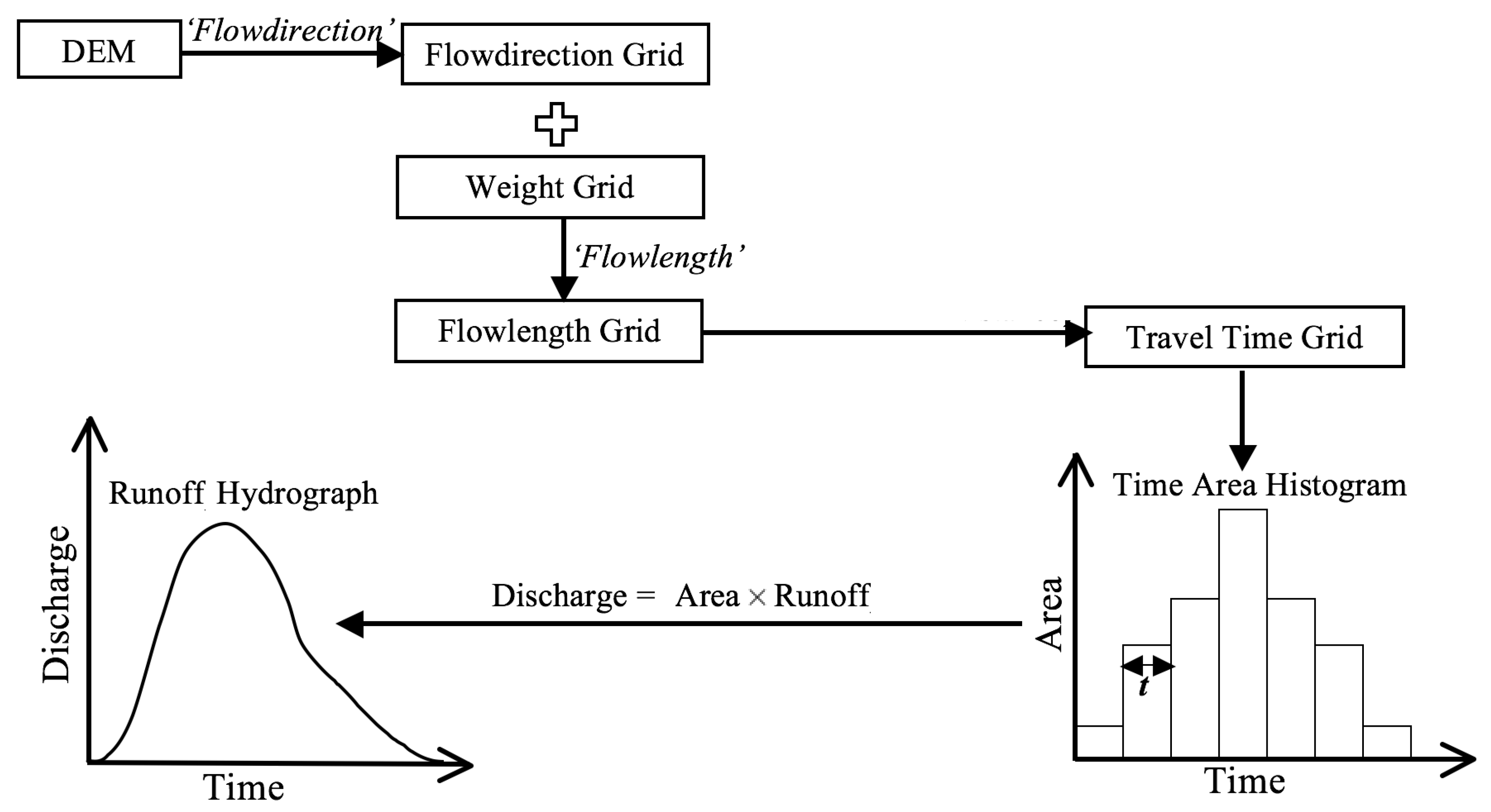
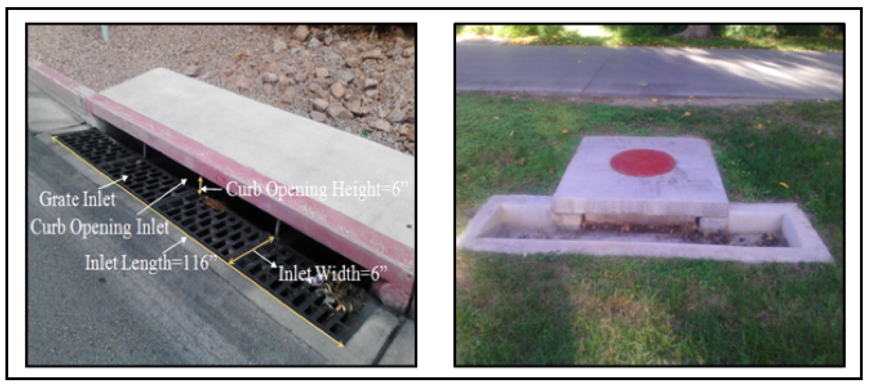
2.3. Runoff to Flow Conversion

The runoff generated through the hydrological model flows to the pour point. There are two mathematical approaches for routing runoff i.e., stochastic method [30,31] and deterministic method [32,33]. Both approaches have been successfully investigated for runoff routing. It is generally considered that stochastic methods are more complex than the deterministic methods. This GIS framework can be plugged-in with any approach of choice and in this research, deterministic approach using travel time is used.

Flow routing involves estimating travel time of runoff from each point in the watershed to the point of interest [27]. Travel time ($T_t$) is difficult to estimate, and can be subjective [22]. There are various methods for estimating travel time, such as the SCS Watershed Lag method [22], SCS Velocity method [27], segmental approaches of Time-Area method [22], Kirpich method [34], and Kerby-Hatheway method [34]. The GIS framework should be applicable to any method for runoff to flow conversion. In this research, time-area histogram method is used to estimate flow at the outlet of selected study sites.

The time-area method method estimates the travel-time of each cell, and groups them into regions of equal travel-time called isochrones. Figure 3 shows the time-area approach for creating runoff hydrograph at the watershed outlet (modified from [33]).

The travel-time of each cell is estimated from flow velocity and flow length, i.e., distance between the cell and the watershed outlet. Flow velocity is estimated using a variant of Manning’s equation [35] given by

$$V(x,y)=0.3048\times K(x,y)\times \sqrt{M(x,y)}$$

(4)

where $V(x,y)$ (m/s) is the velocity at each cell that depends on velocity coefficient $K(x,y)$ and surface slope $M(x,y)$ (%). The value of K depends on the type of flow. According to Sorrell and Hamilton [35], there are three types of flow regimes including small tributary ($K=2.1$), waterway ($K=1.2$), and sheet flow ($K=0.48$). Since the K values were developed to provide velocity in ft/s, $0.3048$ is multiplied to convert into m/s units. The travel time is estimated using weighted flow direction algorithm in GIS, where weights are given to each cell based on the local velocity. In this algorithm, cell length weighted by inverse of local velocity gives cell-to-cell travel time which is integrated along the flow path. The resulting value at each cell is the time required by water to travel from the cell to the outlet. The resulting travel time grid is used to construct isochrones, which are regions with same travel time. The area of each isochrone plotted against their respective travel time is called the time-area histogram, which translates a given rainfall into a hydrograph at the outlet (see Figure 3). This hydrograph is also referred to as runoff hydrograph i.e., flows that are plotted at the midpoint of time intervals of the histogram.

This time-area histogram is applied to compute runoff hydrograph for each time step of input rainfall event (represented as hyetograph). The total hydrograph of the complete rainfall event is generated by appropriately shifting and summing all the individual runoff hydrographs.

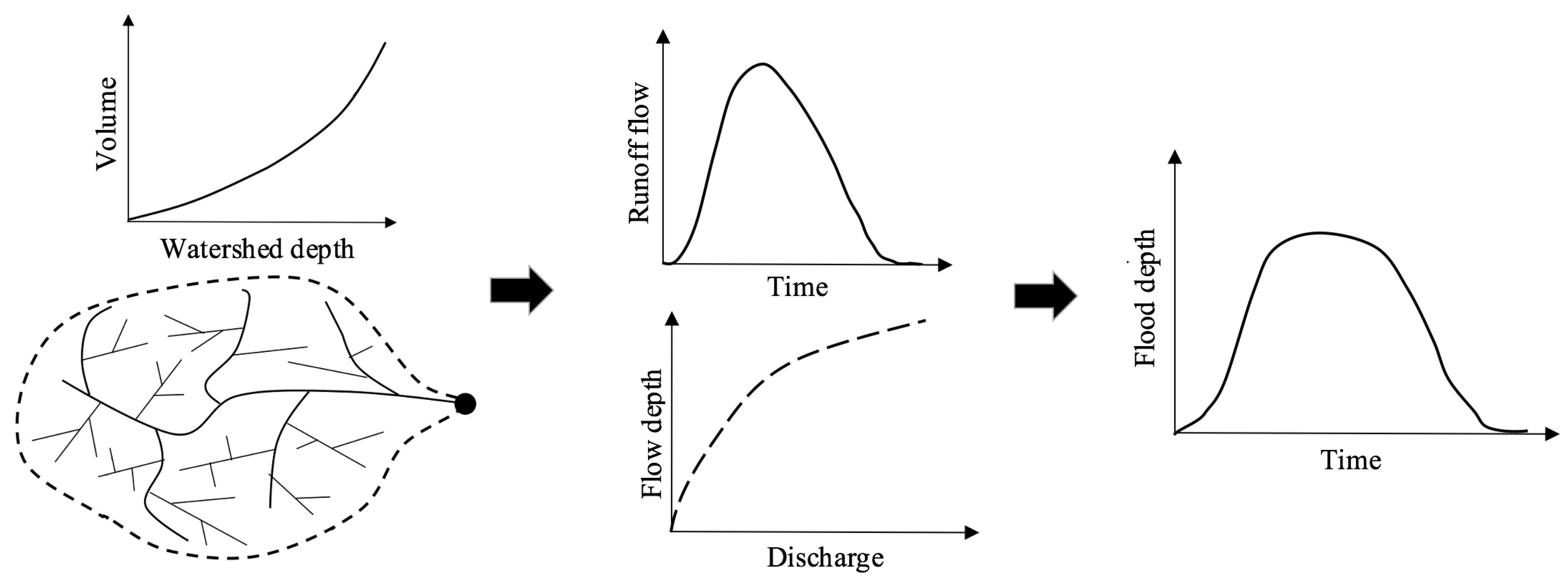
2.4. Inundation Estimation and Mapping

There exist numerous studies on urban flood modeling to estimate inundation characteristics (flood depth, extent, and duration) from a runoff hydrograph [1,5,36,37,38,39]. The most common theme in estimating inundation or ponding is through the application of mass balance. Ponding occurs relatively in low laying areas with no drainage or at the drain inlets with limited discharge capacity. For a given time step, if watershed discharge is greater than the drain inlet discharge capacity, then inundation or ponding occurs. In this process, the low lying areas are first inundated followed by the higher elevations in the proximity. In case of a pour point formed due to no-outlet depression, all runoff contributes to inundation or ponding.

To accurately estimate ponding, it is important to estimate the discharge capacity of the inlet. The discharge capacity of the inlet is estimated by constructing a stage discharge curve also referred to as a rating curve. It exhibits the relationship between the drain inlet’s discharge capacity and upstream flow depth. This rating curve acts as the discharge hydrograph of the inlet. This research follows the processes and equations provided by Guo et al. [40] and UDFCD [41] to estimate the drain inlet capacity. Guo et al. [40] has provided a series of equations applied to estimate discharge capacity of sump type inlets. A sump inlet is any inlet that is located at the lowest point of a drainage area [41]. The operation of an inlet is subject to the clogging due to urban debris that can obstruct the drainage system. It is noted the the equations provided by [40] do not consider clogging effect. In real situation, all the inlets are affected by clogging [41], and hence, a clogging factor should be applied to adjust the inlet capacity. A clogging factor quantifies the effect of obstruction on discharge capacity ranging between 0 (no clogging) and 1(fully clogged) [41]. In this research, the equations of [40] are modified to include clogging factor estimated from [41] for effective discharge capacity of the inlets.

Any flow exceeding the inlet discharge capacity is converted into inundation. Figure 4 shows the inundation estimation process. During a given time interval, the runoff flow arriving at the drain inlet is converted into depth using the stage-volume curve developed from DEM. A stage-volume curve provides information about how much water a watershed can hold for a given depth. To develop the curve, the watershed is treated as a reservoir. The elevation of the watershed cells relative to that of the inlet cell (location) are estimated. The equal-height cells (contours) are used to estimate corresponding storage volume which is plotted against the height to generate stage-volume curve. The flow from the watershed discharge hydrograph is compared to the discharge capacity of the inlet and the flows that exceed the capacity are converted to inundation volume. The inundation volume is converted to depth using the stage-volume curve that are contoured onto the DEM to determine the areal extent of flood.

2.5. Calibration and Validation

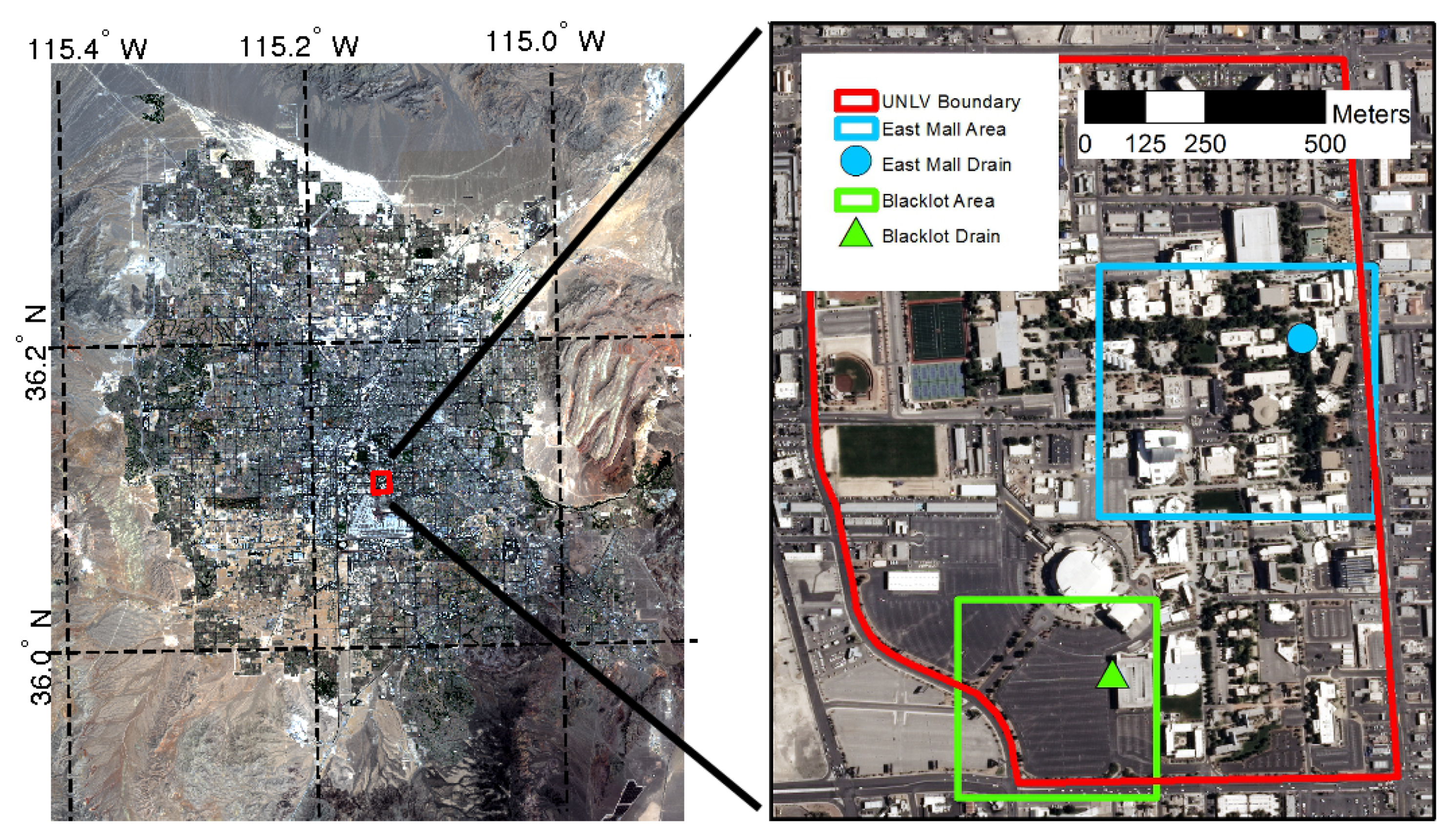
The GIS framework incorporates calibrating and validating the flood mapping model. The flood mapping is achieved through the steps of rainfall to runoff process, runoff to flow process, and inundation estimation process. Calibration and validation generally use observational flow and depth data to adjust parameters of a flood model, and once calibrated, to test the robustness of the model. The parameter calibration can be carried out in two ways, i.e., either by optimizing model performance or through expert knowledge [42]. In both cases, optimization of calibrating parameters is conducted by following a trial and error procedure, where the errors are estimated by various statistical measures, e.g., root mean squared error, mean absolute error, and absolute percent error. The most frequently used approach is the optimization of model performance, which is more appropriate for gauged watersheds. This direct method uses historical flow and depth records for calibration and validation. With an increasing availability of information, various new calibration and validation techniques have been developed such as [43] has used GLUE method combined with Monte Carlo approach. It may not always be feasible to calibrate and validate a model in ungaged watersheds due to lack of historic data. Since many urban micro-watersheds are ungaged lacking sufficient information for calibration and validation, a simple and parsimonious approach can be applied using the local and physical information such as the one reported by [44]. Since flooding in urban areas often occurs rapidly and lasts for short time durations, it is difficult to obtain good historical observations [13]. The calibration in ungauged basins can be achieved through expert knowledge with reasonably good solution [42]. In this case, the visual information of flooding (e.g., satellite images, aerial images, and images captured by a camera) can be used to crosscheck model results. In this indirect method, soft calibration and validation is achieved with data gathered from photographs, newspaper reports, online articles and field visits. These information, if possible, can be divided into two groups where one group of information can be used for calibration and the other one can be used for validation [13].

The five components described above form the GIS-framework. These can be implemented in any GIS application capable of raster processing. In this research, the proposed GIS-based framework is implemented in ArcGIS software, and tested with two flooding cases at UNLV.

3. Case Studies

The two sites, Blacklot and East Mall (Figure 5), located at UNLV main campus experienced flooding on 11 September 2012. Both of the sites discharge runoff to nearby storm inlets shown in the figure. Although there is no historic observational data available, some information about the flood depth and extent at Blacklot is available from photographs and news reports. Therefore, these sites are good candidates to implement the proposed GIS-framework. We implemented the framework inside the computing environment of ArcGIS, and used its embedded Python scripting language for automation. Though this framework uses ArcGIS Python scripting for automation, it can also be built using either the ModelBuilder component or by creating an extension or add-in. Arcmap add-in is a customization including a collection of tools (e.g., plug-ins on the toolbar of ArcGIS Desktop) that provide supplemental functionality to the Arcmap software [45]. In this research, Arcmap add-ins were created using Python interface in the form of library of functions and executable codes. The library builds upon the hydrological processing algorithms in Arcmap Spatial Analyst toolbox and provides tools for the GIS-framework used in this research. Additionally, various executable codes are developed that apply the GIS-framework to a chosen site (e.g., Blacklot or East Mall) with the appropriate choice of algorithms. It is noted that this framework can also be implemented as add-in to the Opensource QGIS software, similar to the implementation of FloodRisk reported by [46].

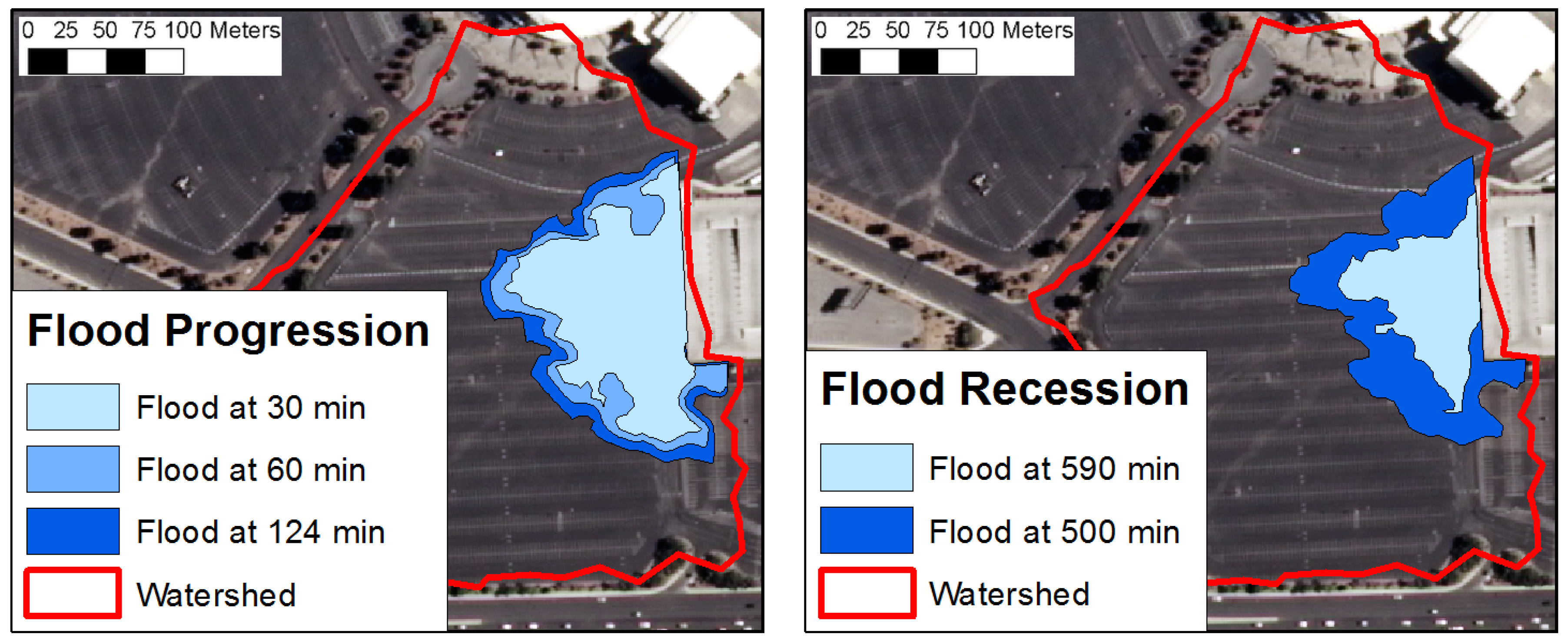
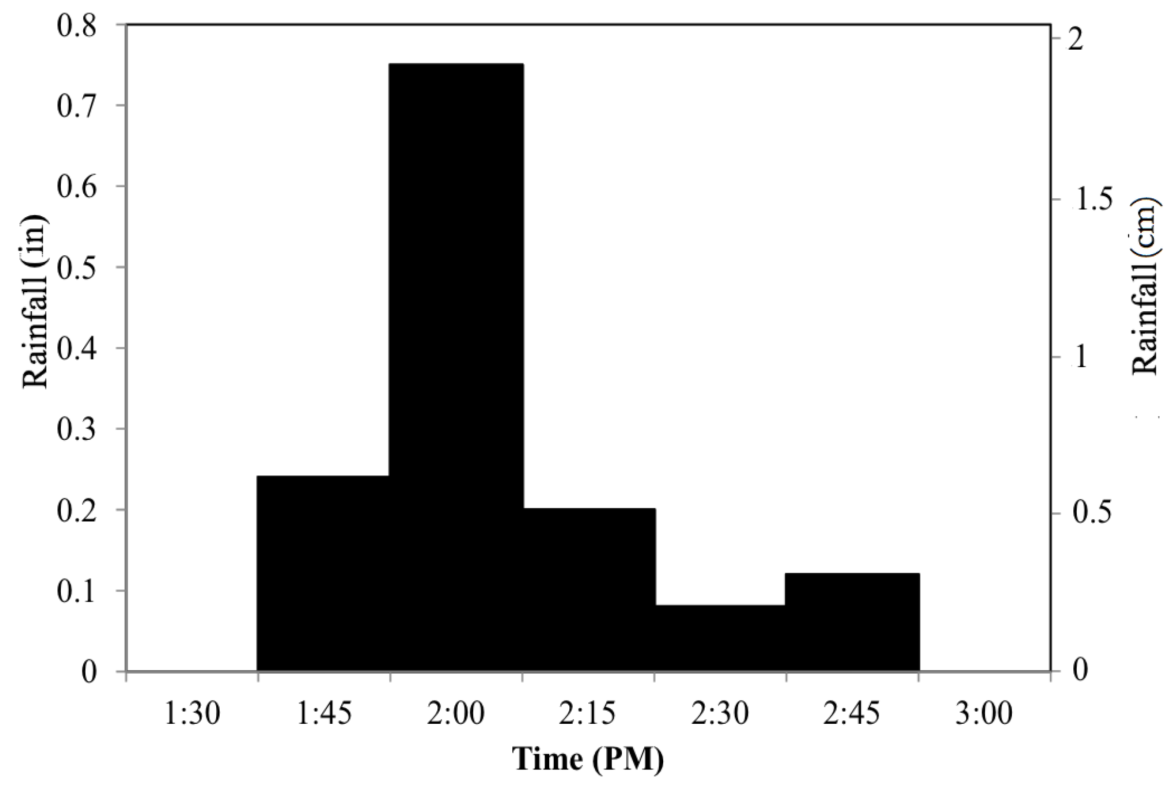
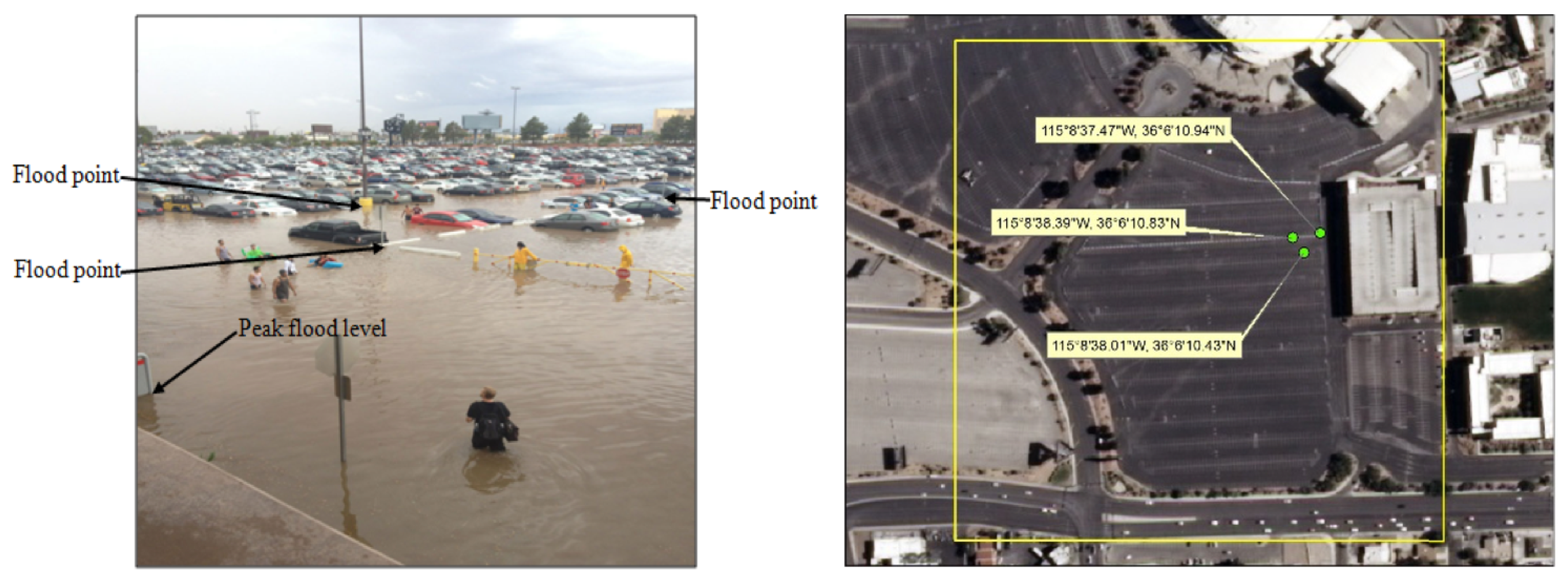
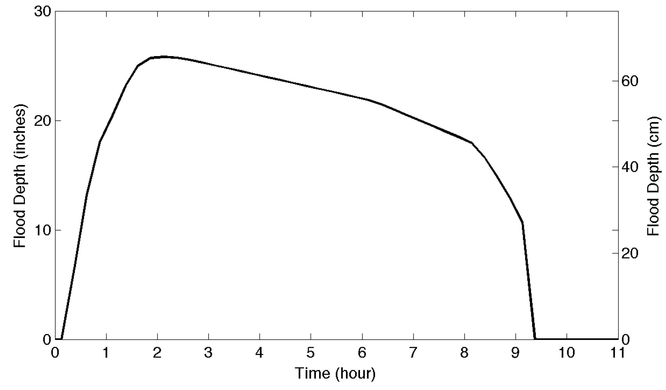
3.1. GIS Framework Testing at Blacklot Study

The Blacklot has a single drainage outlet in the low elevation area, and thus is prone to flooding due to clogging of the inlet or exceedance of design discharge. The surface of the parking lot is asphalt (impervious), and runoff velocity is relatively higher over an impervious surface. With a single drain prone to clogging and high speed runoff, such an area is vulnerable to flash flooding.

The Blacklot storm drain inlet is a street sump type installed along the side of the access road as shown in Figure 6 (left). Figure 6 (right) shows East Mall drain. The Blacklot drain inlet has equal length combination of grate and curb-opening with 116 inches (294.68 cm) length, 18 inches (45.72 cm) width, and 6 inches (15.24 cm) of curb-opening height. This inlet is also a combination type 16 as each segment consists of a vane grate and a curb opening [40]. The following paragraphs describe the specifics of the GIS-based framework for this area.

Watershed Delineation of Blacklot is done using rasterized LiDAR data. The LiDAR point cloud has an average sample spacing of 1.66 m, which was rasterized and analyzed at various spatial resolutions to find the optimal resolution. The LiDAR point cloud consists of multiple returns which are useful when the ground cell contains multiple targets of varying elevation. In this case, we chose the first return which effectively represented surface with sporadic presence of parked vehicles. The erroneous elevations due to these parked vehicles were removed through filtering. LiDAR data was rasterized to create DEM tested at various spatial resolutions. Stream network was constructed and watershed was delineated for each of the DEM resolution. Figure 7 (left) shows the stream network constructed for 1 m resolution DEM, and some watersheds that were delineated by varying the resolution are shown in Figure 7 (right). From the stream network it is apparent that the Blacklot site is separated from the streets by higher ground divides suggesting that the streets have their own stream network for drainage. The watershed boundaries confirm the contributing area of drainage towards the inlet.

Rainfall to runoff conversion is done using SCS-CN method as described in USDA TR-55 manual [27]. In this method, runoff depends on the surface curve number based on soil hydrological group and the land cover class. The hydrological soil group (HSG) data for the study sites were collected from Soil Survey Geographic Database (SSURGO) [47], and the land cover data was collected from National Land Cover Dataset published in 2011 [48]. It is found that the study area has a hydrologic soil group type A, and considered to have developed-medium intensity and developed-high intensity land cover characteristics. The curve number is determined using the conversion table in USDA-TR 55 manual with typical average antecedent moisture condition (AMC II). Blacklot area consists of 86 and 95 curve number surfaces, and thus most of the rainfall becomes runoff. Rainfall data were collected for the flooding day from Clark County Regional Flood Control District (CCRFCD) (http://www.ccrfcd.org/raingauges.htm). The rainfall hyetograph from the nearest station (Station ID: 4574) is used, and shown in Figure 8. This station is also closest to the East Mall study site. It should be mentioned that the total rainfall recorded at this station was 1.38 inches (3.5 cm) which is approximately 35% of the average annual rainfall of the Las Vegas Valley (approximately 4 inches/10.16 cm).

Runoff to flow conversion is done using time area-histogram approach. The hydrograph is calculated for 15-min intervals of the rainfall hyetograph, and accumulated to produce an overall hydrograph for the storm.

The surface slope in Blacklot varies from 0% to 19%, and resulting velocities of the cells range from 0.05 m/s to 0.87 m/s. The higher velocity corresponds to concentrated flow regimes. Figure 9 (top) shows the travel time map of the Blacklot watershed, and Figure 9 (bottom left) shows the corresponding time-area histogram. The longest travel-time to outlet is 129 min. Nine isochrones are produced with a temporal resolution of 15 min. Among these, the 5th isochrone has the largest area (≈30% of watershed area). This isochrone contributes at the outlet after 60 min from the onset of the storm [See Figure 9 (bottom left)]. Figure 9 (bottom right) showing the hydrograph reveals a peak of 2.91 m${}^3$/s occurring after 82 min and runoff ending after 203 min from the beginning of the rainfall. The travel times may seem high for a parking lot with an impervious surface. However, the flood starting time (after 20 min of rainfall) matches to within 5 min of the reported flood starting time at 2:00 pm (after 15 min of rainfall) [49].

Calibration of parameters for the Blacklot is done using flood depth information. In particular, elevation of watermark was collected through field visit that reflects the maximum flooding depth. Three parameters are chosen for calibration in this site including DEM resolution, rainfall temporal resolution, and clogging factor. A DEM of higher resolution captures small elevation details used in stream and watershed delineation. Goulden et al. [50] have concluded that fine-resolution LiDAR-derived DEM offer better results compared to DEM from other sources. Goulden et al. [50] investigated for optimum resolution for LiDAR-derived DEM and emphasized that an optimum DEM resolution is the one that is required for accurate watershed modeling with less computational burden. Determination of optimum DEM resolution depends on matching the resulting streams network, watershed boundaries, and discharge hydrograph to the observational field data. Wang et al. [36] concluded that a rainfall-runoff model performance is greatly influenced by the temporal resolution of hydrologic data, while Aronica et al. [51] also emphasized on considering rainfall resolution as a calibrating parameter in urban drainage modeling. Therefore, rainfall temporal distribution is also considered for calibration in this research. Clogging factor selection mainly depends on the debris and waste in an area during a rainfall event [41]. The amount of urban debris varies with location and season, and therefore clogging factor of an inlet may change every time an analysis is conducted [52]. Conservatively, a clogging factor of 0.5 is recommended for a single grate and 0.1 for a single curb-opening inlet [52]. As clogging factor can significantly impact the performance of a drain inlet, it is considered as a calibrating parameter in this research.

The observed peak flood depth at the inlet is 34 inches (86.36 cm) as observed from maximum water depth marks on signboards (collected from photographs and field visit) shown in Figure 10 (left) [49]. The flooding depth from the watermark was measured, and its location was captured using a GPS instrument. It is noted that the inlet was observed and was almost fully clogged even after the flooding had receded. To calibrate the flood model, the observed peak flood depth is compared with output from the model at various DEM resolutions, rainfall intervals, and clogging factors. The DEM at 5 m spatial resolution produced the lowest error (absolute percent error) of 24%. Moreover, rainfall hyetograph sampled at 15 min produced the lowest error of 24%. The resolutions achieved in the calibration are related to the scale of the hydrological processes captured by the model. In the more common approach, it is achieved by comparing the modeled and observed discharge hydrograph. Since such data is not available in this study site, this model achieved calibration using flooding depth. We conjecture that this choice, i.e., using flood depth for calibration, could be related to the outcome (lowest error) at 5 m DEM and 15 min hyetograph resolutions. Additionally, it may be attributed to the data reconditioning algorithms i.e., filtering and filling used for delineating watershed boundary. A higher DEM resolution may lead to watershed that represents a subcatchment (smaller than the parking lot) whereas a lower resolution may lead to the supercatchment (larger than the parking lot). Ghaffari [53] has reported that the hydrological results vary with watershed area delineated from the DEM. Therefore, a good approximation of model output also relies on accurate watershed area delineation. For this site at 5 m DEM resolution, the drain inlet is most closely aligned with the stream network compard with other DEM resolutions, and hence generates the watershed with accurate parking lot coverage. For the 5-m DEM and 15 min rainfall interval the model-clogging factor is calibrated to reduce the error to 0.72% at 0.83.

Inundation estimates were computed from the runoff hydrograph and the stage-discharge curve of the drain inlet. The effective discharge capacity of the drain inlet at the maximum allowable water depth of 6 inches (15.24 cm) is 11.82 ft${}^3$/s (0.33 m${}^3$/s). The results reveal (see Figure 11) that flooding started after ≈20 min and lasted for several hours. The areal extent is also determined from flood depth by creating contours on the DEM (See Figure 12). Inundated areas at 30, 60, 124, and 500 min are 11,172, 14,672, 17,834 (peak flood), and 13,855 m${}^2$, respectively. While the model is calibrated using the flood depth information, the validation is performed using the geographic locations of the flood points shown in Figure 10 (right) and the flood starting time information. It is found that the points are within the computed inundation extents, and the flood starting time match closely with the reported flood beginning time (≈5 min) confirming the usefulness of the model for this site.

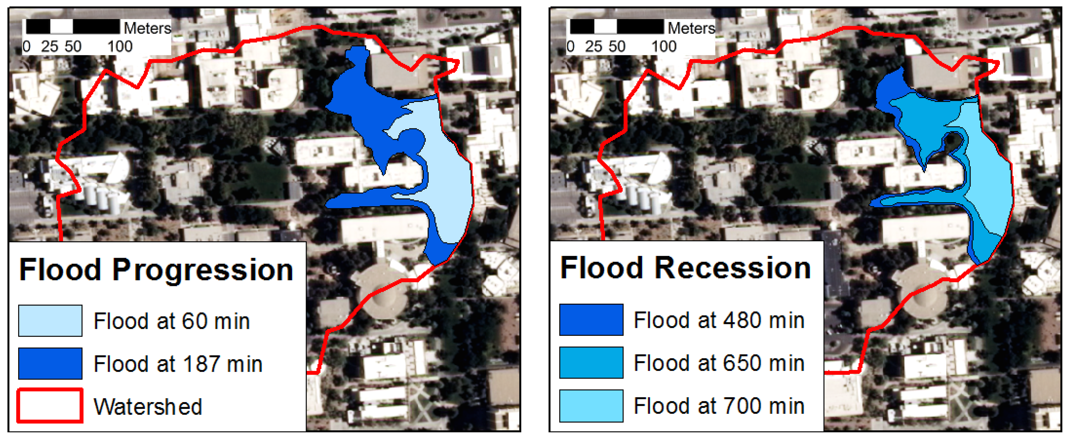
3.2. GIS Framework Testing at East Mall Study Site

The East Mall is located on the east side of the UNLV campus. The area serves as a site for many student functions as well as campus tours, receptions, and conferences. This area is dominated with vegetation as shown in Figure 5, and also has asphalt (parking areas), concrete (buildings) and gravel. The drain inlet of this study site is a curb opening sump inlet type. It is 42 inches (106.7 cm) long with a curb-opening height of 6.5 inches (16.5 cm), and is identical to the R type curb-opening inlet [52]. A GIS-based framework similar to Blacklot is applied, and some specifics are described below.

Stream networks were constructed, and watersheds were delineated for different resolutions of DEM. The DEMs were constructed from the same LiDAR data points similar to that for Blacklot. Although Blacklot does not have any effect of buildings, East Mall has several rooftop catchments contributing to the flow. The buildings in micro-watersheds are fixed obstacles that effect flow in two ways. Firstly, the flow from higher elevations upstream of the building is routed around the buildings through steets. Secondly, the rainfall on rooftop concentrates at roof drains before reaching the ground. The first effect of buildings is captured reasonably by the LiDAR-based DEM showing stream network that primarily follows street network. The second effect is difficult to capture accuratly without additional information of drainage system from roofs. In this research, DEM data captures well the flow behavior around the buildings. The flow from building rooftop is based on flow directions computed from DEM elevations only as roof drainage information is not available. The general slope and aspect of roofs are used in estimating flow behavior, and hence, captured in the stream network by connecting flow from the buildings to the street network. Thus, there is no dependence on the general topographic gradient caused by high building elevation for generating stream network; however, the high gradients can result in very high slope and velocity. Additionally, buildings cause rain shadows as well as alter the prevailing wind regimes.

The study area consists of hydrologic soil group of A, and consists of open spaces developed with high, medium, and low intensity land cover types. Thus, there exist four different curve number values of 49, 66, 86 and 95. The slope in East Mall ranges from 0% to 28%, and flow velocities from 0.15 m/s to 6.36 m/s are observed. The high slopes (that also result in high velocities in Equation (4)) are introduced from high building elevations. These high slope cells represent the flow from the buildings through roof drains. Since the roof drain information was not available and difficult to capture in the model, the slope of these cells are adjusted to match closely to the neighboring cells. The updated values are later used to estimate travel time. The time of concentration is estimated as 210 min, and there exist 14 isochrones with a temporal resolution of 15 min. Among these, the 7th isochrone has the largest area (≈10% of watershed area) that contributes at the outlet after 75 min of rainfall. The peak of the hydrograph is 0.99 m${}^3$/s, and the time to peak is 120 min from the beginning of the rainfall. For calibration, DEM of 5 m produced vey high peak depth error of 100%, and a 1 m DEM produces the lowest error of only 5%. Calibration using rainfall temporal resolution is observed to have the similar impact as for the Blacklot producing the lowest error of 5%. Calibration against clogging factor is not performed as it is a single curb opening inlet and there is an established recommended value of 0.10 [41]. In inundation estimation, the effective discharge capacity of drain inlet at the maximum allowable water depth of 6.5 inch (16.5 cm) is 4.45 ft${}^3$/s (0.126 m${}^3$/s). Flooding started after 52 min of the beginning of rainfall, and ended after 745 min of rainfall resulting in a flood duration of 690 min. Similar to the Blacklot study site, flood depths are contoured in GIS to produce the inundation extents shown in Figure 13. Since there is no reported flood beginning time information available for this site, only the flood extent points (collected using GPS) are compared with the computed inundation extents to validate the model. These GPS locations are within the inundation extent. The flow propagation of flood water is hindered by the buildings, and hence, the flow movement occurred around the buildings [36].

4. Discussion

The GIS-based modeling framework proposed has provided reasonable results at the case study sites. In this section, we discuss certain factors of observation necessary for successful implementation.

Watershed delineation for a specific drain inlet can be challenging if it is not spatially aligned to the stream network. Despite accurate stream network delineation, the drain inlet offset from a stream results in an erroneous watershed boundary. The reason for this is that the location of the drain inlet on the secondary stream is not captured in the stream network. To avoid this problem, the threshold for stream identification can be reduced to include the appropriate stream in the network. Another way, somewhat less accurate but providing reasonable results, is shifting the pour point (also called snapping) onto the closest stream in the stream network.

The rainfall to runoff conversion can be performed with any model of choice. In case of the SCS Curve Number method, care should be exercised when choosing initial abstraction which includes infiltration, evaporation and other losses. In case of an impervious surface such as Blacklot, there is no infiltration, and thus, a different value is applicable. Besides, there should only be a negligible amount of evapotranspiration losses as a very small amount of evaporation is found in such urban watersheds (only 0.003% of the total watershed area) [5]. These factors can result in an overestimation of abstraction resulting in erroneous runoff estimation.

Often it is difficult to acquire the data for model calibration and validation, and thus to assess the accuracy of spatiotemporal behavior of flooding. The post-flooding watermarks often remain intact for several days and can be used to determine the full flood extent. The inherent consistencies of the spatial nature of flooding could ensure such soft calibration and validation to produce results as observed in Blacklot and East Mall.

The analysis of results also show that the common notion that models using higher resolution DEM would provide higher accuracy is not always applicable. For the Blacklot study site it is observed that 5-m DEM produced the smallest error while 8-m DEM produced the largest error. For the East Mall study site, a 1-m DEM produced the smallest error. It is noted that the choice of DEM resolution interplays with other available geographic information such as location of the pour point and land cover in determining overall accuracy. Similarly, the rainfall hyetograph interval size was also varied and showed increasing error at higher temporal resolutions. The clogging factor for the calibrated model in Blacklot is 0.83 which may seem high. This result shows that significant clogging occurred which was also reported by another source [54].

5. Summary and Conclusions

This research develops a GIS-based framework to model and map spatiotemporal variation of flooding in urban micro-watersheds draining into storm drain inlets. A methodology is proposed that consists of five components including watershed delineation, rainfall to runoff conversion, runoff to flow conversion, inundation estimation and mapping, and calibration and validation. This framework is a workflow with steps that can be completed using physical and empirical approaches eligible to be deployed inside a GIS computing environment with raster processing capabilities. This framework was tested at two urban sites including an impervious parking lot (Blacklot) and a pervious vegetated surface (East Mall). Watershed delineation was done using DEM data from LiDAR for specific drain inlets. Rainfall is converted to runoff using the SCS-CN method using SSURGO soil data and NLCD land cover data. Runoff is converted to flow at the drain inlet using the time-area histogram method. The runoff hydrograph at the drain inlet is compared to the stage-discharge curve of the drain to estimate inundation depth, peak, and extent. These inundation results are compared with the observed data for calibration and validation. The results show that the DEM of 5 m resolution produced an accurate watershed response for the Blacklot while 1 m produced accurate results for the East Mall. A clogging factor of 0.83 and 0.10 is estimated for Blacklot and East Mall, respectively. The spatiotemporal behavior produced by the proposed GIS-framework is consistent with news reports and post-flood observations. This GIS-framework developed in the research is useful for spatiotemporal modeling and mapping of urban floods. This GIS-framework is a guideline for flood modeling and mapping with a choice of plugging-in varying methods to execute individual steps.

The proposed framework is a workflow of methods for flood modeling and mapping in urban watersheds draining to storm drain inlets. The advantage of this framework is its ease of implementation in a GIS software. The framework also provides flexibility of implementing different methods for each component. For example, the rainfall to runoff component can be implemented by other methods such as Green-Ampt infiltration model. Although the framework is implemented in ArcGIS software, it can be implemented in other compatible commercial and Opensource GIS software (e.g., Quantum GIS) as well. ArcGIS and QGIS (with GRASS) provide vector and raster toolboxes for hydrologic analysis such as computation of flow direction, flow accumulation, and flow length. Moreover, ArcGIS has capability for automation of the processing using built-in Python language scripting interface. The simplistic layout of this framework is also a limitation as it cannot capture complex models, for example feedbacks of dual drainage systems in urban flooding.

References

1. Jing, Z. GIS based urban flood inundation modeling. In Proceedings of the 2010 Second WRI Global Congress on Intelligent Systems (GCIS), Wuhan, China, 16–17 December 2010; Volume 2, pp. 140–143. [Google Scholar]
2. Zerger, A.; Smith, D.; Hunter, G.; Jones, S. Riding the storm: A comparison of uncertainty modelling techniques for storm surge risk management. Appl. Geogr. 2002, 22, 307–330. [Google Scholar] [CrossRef]
3. Genovese, E. A Methodological Approach to Land Use-Based Flood Damage Assessment in Urban Areas: Prague Case Study; Technical EUR Reports; European Commission: Luxembourg, 2006. [Google Scholar]
4. Feyen, J.; Shannon, K.; Neville, M. Water and Urban Development Paradigms: Towards an Integration of Engineering, Design and Management Approaches; CRC Press: Boca Raton, FL, USA, 2008. [Google Scholar]
5. Chen, J.; Hill, A.A.; Urbano, L.D. A GIS-based model for urban flood inundation. J. Hydrol. 2009, 373, 184–192. [Google Scholar] [CrossRef]
6. Kilgore, J.L. Development and Evaluation of a GIS-Based Spatially Distributed Unit Hydrograph Model. Ph.D. Thesis, Virginia Polytechnic Institute and State University, Blacksburg, VA, USA, 1997. [Google Scholar]
7. Shokoohi, A.R. A new approach for isochrone mapping in one dimensional flow for using in time area method. J. Appl. Sci. 2008, 8, 516–521. [Google Scholar] [CrossRef]
8. Urbonas, B. Stormwater Runoff Modeling; Is it as Accurate asWe Think? In Proceedings of the International Conference on Urban Runoff Modeling: Intelligent Modeling to Improve Stormwater Management, Arcata, CA, USA, 22–27 July 2007; p. 12. [Google Scholar]
9. Leandro, J.; Chen, A.S.; Djordjević, S.; Savić, D.A. Comparison of 1D/1D and 1D/2D coupled (sewer/surface) hydraulic models for urban flood simulation. J. Hydraul. Eng. 2009, 135, 495–504. [Google Scholar] [CrossRef]
10. Fraga, I.; Cea, L.; Puertas, J. Validation of a 1D-2D dual drainage model under unsteady part-full and surcharged sewer conditions. Urban Water J. 2017, 14, 74–84. [Google Scholar] [CrossRef]
11. Hsu, M.H.; Chen, S.H.; Chang, T.J. Inundation simulation for urban drainage basin with storm sewer system. J. Hydrol. 2000, 234, 21–37. [Google Scholar] [CrossRef]
12. Chen, A.S.; Evans, B.; Djordjević, S.; Savić, D.A. A coarse-grid approach to representing building blockage effects in 2D urban flood modelling. J. Hydrol. 2012, 426, 1–16. [Google Scholar] [CrossRef]
13. Wang, Y.; Chen, A.S.; Fu, G.; Djordjević, S.; Zhang, C.; Savić, D.A. An integrated framework for high-resolution urban flood modelling considering multiple information sources and urban features. Environ. Model. Softw. 2018, 107, 85–95. [Google Scholar] [CrossRef]
14. Ghimire, B.; Chen, A.S.; Guidolin, M.; Keedwell, E.C.; Djordjević, S.; Savić, D.A. Formulation of a fast 2D urban pluvial flood model using a cellular automata approach. J. Hydroinform. 2013, 15, 676–686. [Google Scholar] [CrossRef]
15. Bisht, D.S.; Chatterjee, C.; Kalakoti, S.; Upadhyay, P.; Sahoo, M.; Panda, A. Modeling urban floods and drainage using SWMM and MIKE URBAN: A case study. Nat. Hazards 2016, 84, 749–776. [Google Scholar] [CrossRef]
16. Ellis, J.B.; Viavattene, C. Sustainable urban drainage system modeling for managing urban surface water flood risk. CLEAN Soil Air Water 2014, 42, 153–159. [Google Scholar] [CrossRef]
17. Zhang, Y.; McBroom, M.W.; Grogan, J.; Hung, I. Snapping a Pour Point for Watershed Delineation in ArcGIS Hydrologic Analysis. The Forestry Source, 14 September 2011. [Google Scholar]
18. Horritt, M.; Bates, P. Effects of spatial resolution on a raster based model of flood flow. J. Hydrol. 2001, 253, 239–249. [Google Scholar] [CrossRef]
19. Werner, M. Impact of grid size in GIS based flood extent mapping using a 1D flow model. Phys. Chem. Earth Part B Hydrol. Oceans Atmos. 2001, 26, 517–522. [Google Scholar] [CrossRef]
20. Chen, J.; Hill, A. Modeling urban flood hazard: just how much does dem resolution matter? Pap. Proc. Appl. Geogr. Conf. 2007, 30, 372. [Google Scholar]
21. Prodanović, D.; Stanić, M.; Milivojević, V.; Simić, Z.; Arsić, M. DEM-based GIS algorithms for automatic creation of hydrological models data. J. Serb. Soc. Comput. Mech. 2009, 3, 64–85. [Google Scholar]
22. National Weather Service. Unit Hydrograph (UHG) Technical Manual. 2005. Available online: http://www.nohrsc.noaa.gov/technology/gis/uhg_manual.html (accessed on 7 September 2013).
23. Lindsay, J.B.; Rothwell, J.J.; Davies, H. Mapping outlet points used for watershed delineation onto DEM-derived stream networks. Water Resour. Res. 2008, 44. [Google Scholar] [CrossRef]
24. Craig, J.; Liu, G.; Soulis, E. Runoff—Infiltration partitioning using an upscaled Green—AMPT solution. Hydrol. Process. 2010, 24, 2328–2334. [Google Scholar] [CrossRef]
25. Beven, K.; Robert, E. Horton’s perceptual model of infiltration processes. Hydrol. Process. 2004, 18, 3447–3460. [Google Scholar] [CrossRef]
26. Stall, J.B. Storm Sewer Design—An Evaluation of the RRL Method; US Government Printing Office: Washington, DC, USA, 1972; Volume 1.
27. Cronshey, R. Urban Hydrology for Small Watersheds; Technical Report; US Department of Agriculture, Soil Conservation Service, Engineering Division: Washington, DC, USA, 1986.
28. Yuan, Y.; Nie, W.; McCutcheon, S.C.; Taguas, E.V. Initial abstraction and curve numbers for semiarid watersheds in Southeastern Arizona. Hydrol. Process. 2014, 28, 774–783. [Google Scholar] [CrossRef]
29. Ponce, V.M.; Hawkins, R.H. Runoff curve number: Has it reached maturity? J. Hydrol. Eng. 1996, 1, 11–19. [Google Scholar] [CrossRef]
30. Olivera, F.; Maidment, D. Geographic Information Systems (GIS)-based spatially distributed model for runoff routing. Water Resour. Res. 1999, 35, 1155–1164. [Google Scholar] [CrossRef]
31. De Smedt, F.; Liu, Y.; Gebremeskel, S. Hydrologic Modeling on a Catchment Scale Using GIS and Remote Sensed Land Use Information; WIT Press: Southampton, UK, 2000; pp. 295–304. [Google Scholar]
32. Ashour, R.A. Description of a simplified GIS-based surface water model for an arid catchment in Jordan. In Proceedings of the 20th Annual International ESRI User Conference, San Diengo, CA, USA, 8–12 June 2000; pp. 26–30. [Google Scholar]
33. Usul, N.; Yilmaz, M. Estimation of instantaneous unit hydrograph with Clark’s Technique in GIS. In Proceedings of the 2002 ESRI International User Conference, San Diego, CA, USA, 8–12 July 2002; ESRI On-Line. Available online: http://proceedings.esri.com/library/userconf/proc02 (accessed on 15 December 2018).
34. Thompson, D.B. The Rational Method; Civil Engineering Deptartment, Texas Tech University: Lubbock, TX, USA, 2006. [Google Scholar]
35. Sorrell, R.C.; Hamilton, D.A. Computing Flood Discharges for Small Ungaged Watersheds; Geological and Land Management Division, Michigan Department of Environmental Quality: Lansing, MI, USA, 2003.
36. Wang, Y.; He, B.; Takase, K. Effects of temporal resolution on hydrological model parameters and its impact on prediction of river discharge/Effets de la résolution temporelle sur les paramètres d’un modèle hydrologique et impact sur la prévision de l’écoulement en rivière. Hydrol. Sci. J. 2009, 54, 886–898. [Google Scholar] [CrossRef]
37. Ahmad, M.M.; Ghumman, A.R.; Ahmad, S. Estimation of Clark’s instantaneous unit hydrograph parameters and development of direct surface runoff hydrograph. Water Resour. Manag. 2009, 23, 2417–2435. [Google Scholar] [CrossRef]
38. Ahmad, S.; Simonovic, S.P. Developing runoff hydrograph using artificial neural networks. In Proceedings of the ASCE EWRI Conference-Bridging the Gap: Meeting the World’s Water and Environmental Resources Challenges, Orlando, FL, USA, 20–24 May 2001. [Google Scholar]
39. Ahmad, S.; Simonovic, S.P. An artificial neural network model for generating hydrograph from hydro-meteorological parameters. J. Hydrol. 2005, 315, 236–251. [Google Scholar] [CrossRef]
40. Guo, J.C.; MacKenzie, K.A.; Mommandi, A. Design of Street Sump Inlet. J. Hydraul. Eng. 2009, 135, 1000–1004. [Google Scholar] [CrossRef]
41. UDFCD. Urban Storm Drainage Criteria Manual-Volume 1: Management, Hydrology, and Hydraulics. 2002. Available online: http://udfcd.org/volume-one (accessed on 15 December 2013).
42. Brath, A.; Montanari, A.; Moretti, G. Assessing the effect on flood frequency of land use change via hydrological simulation (with uncertainty). J. Hydrol. 2006, 324, 141–153. [Google Scholar] [CrossRef]
43. Inam, A.; Adamowski, J.; Prasher, S.; Albano, R. Parameter estimation and uncertainty analysis of the Spatial Agro Hydro Salinity Model (SAHYSMOD) in the semi-arid climate of Rechna Doab, Pakistan. Environ. Model. Softw. 2017, 94, 186–211. [Google Scholar] [CrossRef]
44. Albano, R.; Sole, A.; Adamowski, J.; Perrone, A.; Inam, A. Using FloodRisk GIS freeware for uncertainty analysis of direct economic flood damages in Italy. Int. J. Appl. Earth Obs. Geoinf. 2018, 73, 220–229. [Google Scholar] [CrossRef]
45. ESRI. What Is a Python Add-In? 2019. Available online: http://desktop.arcgis.com/en/arcmap/latest/analyze/python-addins/what-is-a-python-add-in.htm (accessed on 13 January 2019).
46. Albano, R.; Mancusi, L.; Sole, A.; Adamowski, J. FloodRisk: A collaborative, free and open-source software for flood risk analysis. Geomat. Natl. Hazards Risk 2017, 8, 1812–1832. [Google Scholar] [CrossRef]
47. NRCS. Soil Survey Geographic Database (SSURGO). 2013. Available online: http://websoilsurvey.sc.egov.usda.gov (accessed on 9 September 2013).
48. USGS. National Land Cover Dataset (NLCD). 2011. Available online: http://www.mrlc.gov (accessed on 8 September 2013).
49. Pridgon, F. Flash Floods Hit UNLV, Many Stranded. 2012. Available online: https://www.unlvfreepress.com/flash-floods-hit-unlv-many-stranded/ (accessed on 7 September 2013).
50. Goulden, T.; Hopkinson, C.; Jamieson, R.; Sterling, S. Sensitivity of watershed attributes to spatial resolution and interpolation method of LiDAR DEMs in three distinct landscapes. Water Resour. Res. 2014, 50, 1908–1927. [Google Scholar] [CrossRef]
51. Aronica, G.; Freni, G.; Oliveri, E. Uncertainty analysis of the influence of rainfall time resolution in the modelling of urban drainage systems. Hydrol. Process. 2005, 19, 1055–1071. [Google Scholar] [CrossRef]
52. Guo, J.C.Y.; MacKenzie, K. Hydraulic Efficiency of Grate and Curb-Opening Inlets under Clogging Effect; Technical Report; Colorado Department of Transportation, DTD Applied Research and Innovation Branch: Denver, CO, USA, 2012.
53. Ghaffari, G. The impact of DEM resolution on runoff and sediment modelling results. Res. J. Environ. Sci. 2011, 5, 691–702. [Google Scholar] [CrossRef]
54. Formoso, J.A. Local Businesses on the Rebound after ‘The Great Flood’. 2013. Available online: https://www.unlvfreepress.com/local-businesses-on-the-rebound-after-the-great-flood/ (accessed on 5 September 2013).
Figure 1. GIS framework for spatiotemporal flood modeling and mapping.
Geosciences 09 00077 g001
Figure 2. Urban watershed delineation in GIS.
Geosciences 09 00077 g002
Figure 3. Runoff hydrograph construction using time-area approach.
Geosciences 09 00077 g003
Figure 4. Graphical representation of inundation estimation process; typical runoff hydrograph (upper middle side); inlet stage-discharge curve (lower middle side); stage-volume curve (upper left corner); and flood depth vs. time curve (right corner).
Geosciences 09 00077 g004
Figure 5. Map showing Blacklot and East Mall study sites.
Geosciences 09 00077 g005
Figure 6. Storm drain inlet in Blacklot study site (on the left) and East Mall study site (on the right).
Geosciences 09 00077 g006
Figure 7. Stream network constructed using 1 m DEM for the Blacklot is shown (on the left), while watersheds for the inlet generated from different DEMs are shown (on the right).
Geosciences 09 00077 g007
Figure 8. Rainfall Hyetograph for the flood event on 11 September 2012.
Geosciences 09 00077 g008
Figure 9. Figure showing travel time map (on the top), time area histogram (on the bottom left), and runoff hydrograph (on the bottom right) of the Blacklot watershed.
Geosciences 09 00077 g009
Figure 10. Imagery used for model calibration showing the location of some of the known flood points and the peak flood depth location at the inlet where watermark was still intact after flooding (on the left) verified through a field visit, and the exact geographic location of the points recorded via field visit with a GPS (on the right). Courtesy of Rebel Yell, University of Nevada Las Vegas.
Geosciences 09 00077 g010
Figure 11. Flood depth variation over time in the Blacklot watershed.
Geosciences 09 00077 g011
Figure 12. Spatiotemporal map of inundation at Blacklot.
Geosciences 09 00077 g012
Figure 13. Spatiotemporal map of inundation at East Mall.
Geosciences 09 00077 g013