1. Introduction
As the water sector moves into the digital era it is inevitable that detailed hydraulic models will be used for real-time monitoring, forecasting and real-time control purposes. Up to now, the use of real-time models in the sector is mostly limited to simplified linear models for model predictive control [
1], but as the number of sensors in the systems increases along with the available computational power, both the requirements and possibilities change. Distributed hydrodynamic urban drainage models (DUDMs), such as SWMM, MIKE URBAN and InfoWorks, can potentially relate to all observations from the system and can therefore be used to make model-based inferences about the state of the system, as well as model-based cross-validation of sensors.
The surface runoff processes in DUDMs are typically lumped-conceptual at the sub-catchment scale, while the flow and water levels in the pipe system throughout the model area are modeled in a physically distributed way by solving the full 1D St. Venant equations. Thereby, DUDMs can be used to keep track of the overall water balance of the system and to estimate overflow from the sewer system to recipients, as well as to estimate flooding in streets and basements. The complexity of the hydraulic calculations allows DUDMs to simulate the flow conditions during surcharge caused by water backing up in the pipe system. This situation occurs in most drainage systems during rain events, for example in connection with combined sewer overflow structures (CSOs) where an orifice or throttle pipe introduces a flow constraint, and the water level is allowed to increase until it reaches the crest level of the overflow weir.
Utility companies put a lot of effort into creating true-to-life detailed DUDMs, but even the best models are not perfect since the dominating inputs to the models are rainfall estimates that will always be uncertain. For an online DUDM to be useful it is required that its physical states can be updated from system measurements to match current conditions. However, the only implemented updating method that is currently available off-the-shelf for DUDMs is based on deterministic point-wise updating [
2], and this does not utilize the full potential of modern data assimilation (DA) schemes. Experimental methods have been proposed for updating the states of the hydrological parts of DUDMs [
3,
4] but these methods only indirectly update the states of the hydrodynamic part of the model, do not produce uncertainty estimates, and will be difficult to use in a general case with data from multiple gauges.
DUDMs are highly non-linear and may include thousands of physical state variables; they are therefore computationally costly. Models with such characteristics are often updated with variants of the Ensemble Kalman Filter (EnKF) [
5] within related fields such as stream flow forecasting [
6] and weather forecasting [
7], since it has proven to be robust towards non-linearities and non-Gaussian errors [
8]. Furthermore, it has been shown that the method works for DUDMs in the case of assimilating observations from a single flow or water level gauge [
9]. The EnKF is a Monte Carlo implementation of the extended Kalman filter in which the error statistics required for computing the Kalman gain (a matrix that determines how much each state in a model is corrected in response to a given deviation between the model and observations) are derived from an ensemble of models that are propagated forward in time in parallel. This approach is more efficient for large non-linear models than non-ensemble based Kalman filters [
5]. Furthermore, research has shown that the EnKF can even be used to utilize information from range-limited observations when the observed quantity is outside the observable range of the gauge [
10], which is a very common situation for gauges in urban drainage systems.
Propagating a large ensemble of DUDMs forward in time is computationally expensive and this may have hampered the breakthrough of the EnKF as a DA method for these models. In order to reduce the computational burden, the EnKF is sometimes used offline to estimate a gain that can be regarded to be constant in time, e.g., [
11,
12,
13,
14]. The constant Kalman gain can then be used in the online situation to correct the model via the standard Kalman filter state update equation, which simply implies to increment the state vector with the product of the Kalman gain and the measurement residual (the difference between observed and modeled values) whenever observations are available. This eliminates the need for an online ensemble, but it is possible only if the Kalman gain can be assumed to be approximately constant in time, which, as we show in the following, is not the case for urban drainage systems exposed to surcharge. Here, we document through a synthetic experiment for a single pipe stretch with a downstream CSO structure, that the Kalman gain varies dynamically in both time and space during backwater periods, and this critical finding should be taken into account when developing future DA schemes for DUDMs.
2. The Ensemble Kalman Filter
In the EnKF each of the ensemble members are updated using the standard Kalman filter (KF) analysis equation:
where
xa is the analyzed model state,
xb the background state (model prediction from the previously analyzed state),
d a vector containing observations, and
H a matrix that relates the model states to the observations.
K is the Kalman gain, which determines how much each state in the model (ensemble member) should be corrected from a given residual deviation between model and observation. In the standard Kalman filter
K is calculated from the forecasted error covariance matrix
Pb:
where
R is the covariance matrix of observation errors. For large models with tens or even hundreds of thousands of state variables, as will usually be the case with DUDMs, it would be extremely expensive to propagate this matrix forward in time analytically as is done in the standard KF. Therefore, the standard KF, or its non-linear equivalent the extended KF, is not an option for DUDMs. The main idea behind the EnKF is to replace the error covariance in Equation (2) with the ensemble covariance. This allows for much more efficient calculation of
K since it can be computed directly from the ensemble without explicitly calculating the ensemble covariance, as described by [
15]. The specific EnKF implementation used in the current study is part of a generic experimental data assimilation framework for all members in the MIKE simulation software family. This has previously been used to update hydraulic head in groundwater models [
16].
3. Experiment
The DUDM used in the current study is a MIKE URBAN [
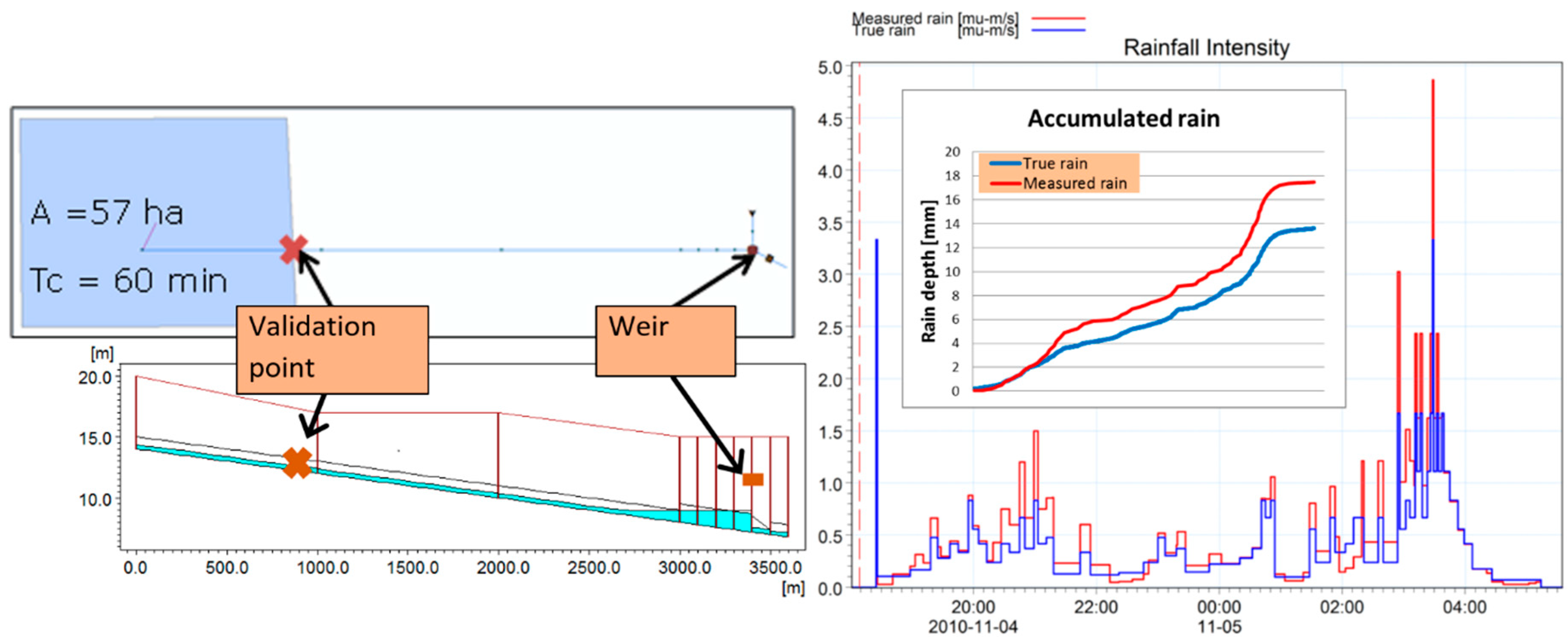
17] model of a 3.4 km pipe stretch with a 1.8‰ slope and diameters in the range of 1–1.5 m, leading to a downstream overflow structure with a 0.4 m throttle pipe and a weir-crest at 12.0 m elevation, see
Figure 1 (left). The observation point is placed at the weir and a validation point is placed 2.5 km upstream from the weir to investigate how updating affects upstream model locations. The inflow to the pipe stretch is created by a simple time-area model with an impervious area of 57 ha, a 60 min time of concentration and a wastewater flow of 10 L/s. During low flows all water runs through the throttle pipe, but when the flow into the structure supersedes the capacity of the throttle pipe, the water level rises and backs up into the pipe system until a maximum extent controlled by the crest level of the weir. A model time step size of 1 s is used, which is sufficiently small to avoid most numerical instability problems with this type of model.
Since the EnKF works by analyzing and manipulating a state vector, it is necessary to construct a suitable state vector from the variables of the model. In DUDMs the routing of water is modeled by solving the full dynamic wave formulation of the 1d Saint-Venant equations. These equations are solved using finite difference schemes of alternating water level and discharge points, which means that the full state of the model contains both water level and discharge variables. Changes to the discharge variables do not, however, change the volume or distribution of the water in the model, and we therefore decided to include the water levels only in the state vector used for the EnKF updating. The state vector consists of a total of 65 water level variables.
The experiment is a perfect model experiment in which a DUDM is used to create both a synthetic truth and synthetic measurements. A rainfall data time series is chosen to represent the true rain, from which true water level observations in the system are generated using the DUDM (blue curves in
Figure 1, right panel). The “true” rainfall time series is then perturbed in order to create synthetic rainfall measurements. The water level observations are created by adding uncorrelated white noise with a standard deviation of 0.1 m to the true water level. The sensor is assumed to have the properties of an ultrasonic level sensor, since this is the most common type of sensor in most drainage systems. The magnitude of the errors from this sort of sensor is usually not dependent on the water level, meaning that it is reasonable to represent the errors as additive noise. This makes it easier to interpret the causes to changes in the Kalman gain than if multiplicative observation noise had been used. A water level observation is created for each EnKF update which is performed at one- minute intervals.
To describe the rainfall uncertainty in the EnKF an ensemble of 20 rainfall time series is created by multiplying the true rainfall data with a random, uniformly distributed number between 0.1 and 1.9 that is drawn at random time intervals between 1 min and 60 min. This noise formulation has been chosen in order to depict something we believe resembles the errors from radar rainfall estimates which are not likely to be the Gaussian noise that is the optimal for Kalman filter implementations. The temporal persistence in the rainfall errors results in spatial correlations in the errors in the pipe system and therefore has an influence on the model updating.
The model setup replicates a very common setup in most sewer systems but is simplified to fit the purpose of this investigation. By using a single catchment only as input to the pipe system the impact of the spatial variability of the rainfall is eliminated, which otherwise could affect the Kalman gain and make it difficult to investigate the courses of the gains behavior. The models are assumed to be perfect, which implies that there are no model errors in the experiment, thus all errors arise from the rainfall and water level observation errors, and these are completely uncorrelated.
When using the EnKF, it is not necessary to compute the Kalman gain explicitly. This is, however, done in the following in order to illustrate the non-uniform dynamic behavior of the gain.
4. Results and Discussion
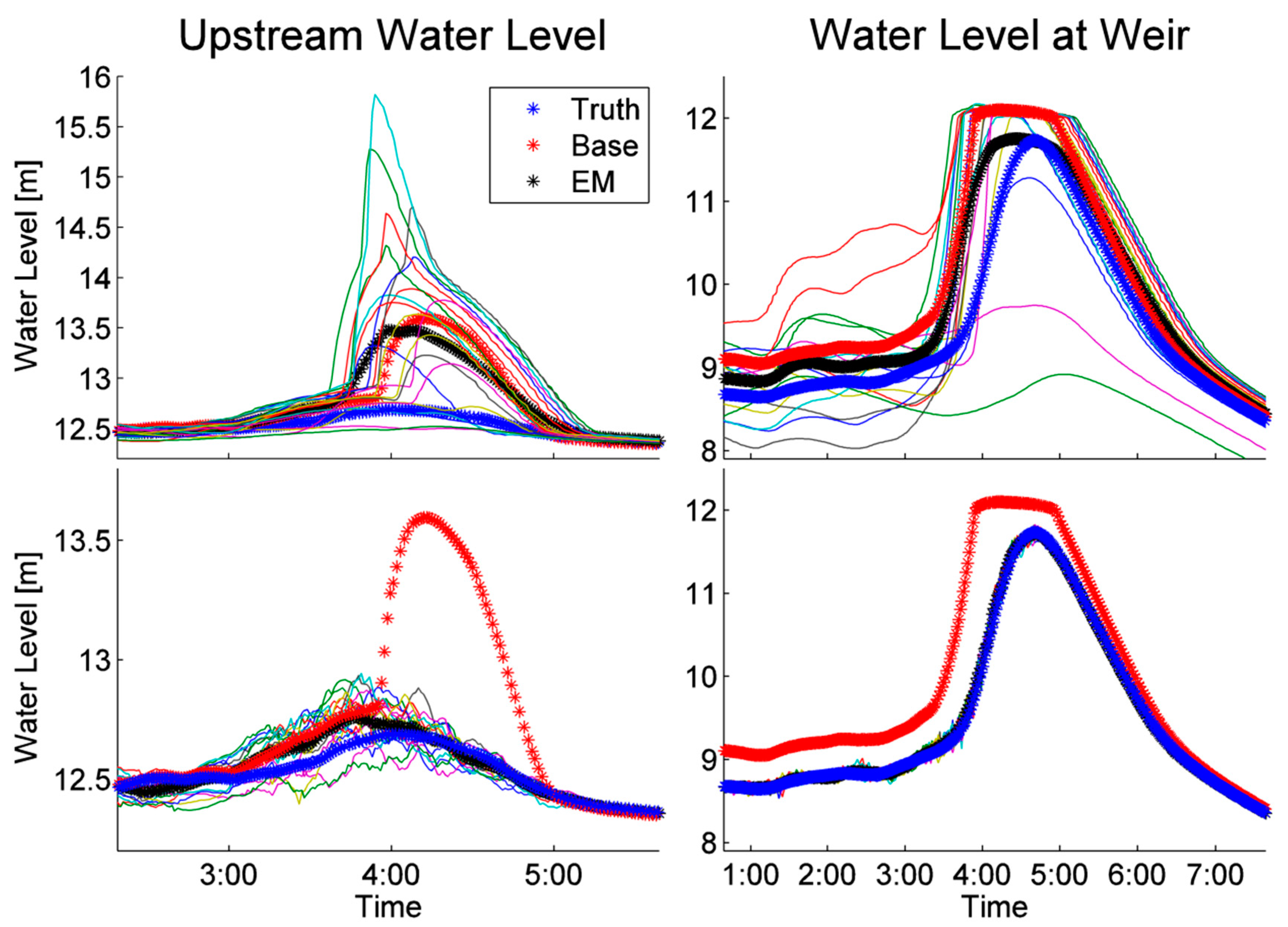
The results of propagating the true and measured rainfall, as well as the 20 realizations of the rainfall through the model, are shown in
Figure 2, in terms of modeled water levels at the weir and the upstream validation point. The model, forced with measured rainfall (base model) as well as most of the ensemble members, vastly overestimates the water levels when updating is not activated (upper panels of
Figure 2). When the ensemble members are updated (lower panels), they are closely centered around the truth at the observed location (at the weir) as well as at the upstream validation point. This shows that the updating works well, and thereby also that the Kalman gain used for the updating is appropriate.
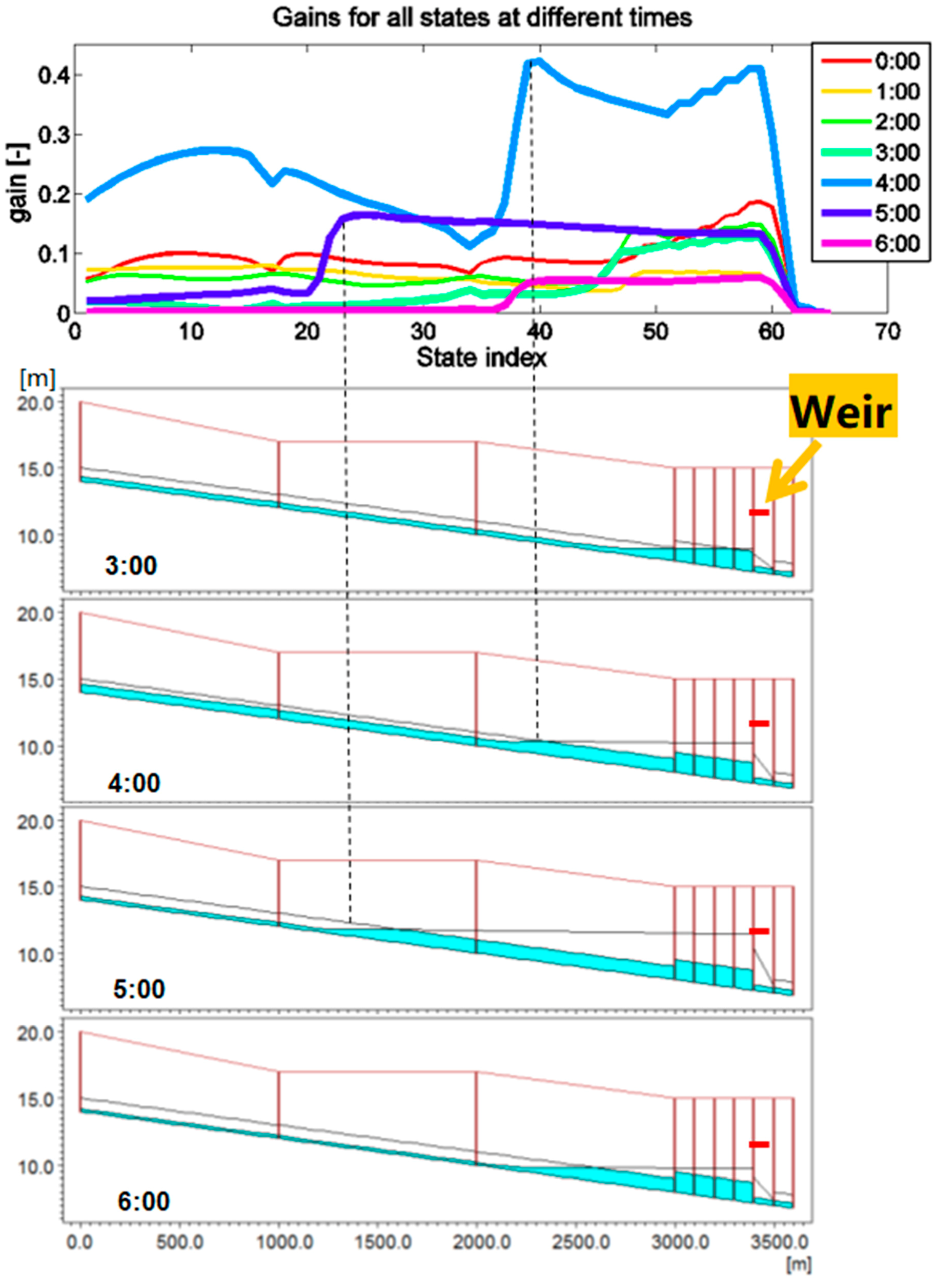
Figure 3 (upper panel) shows the computed Kalman gain for every hour from 00:00 to 06:00, i.e., a period during and after the occurrence of the most intense rainfall, cf.
Figure 1 (right).
Figure 3 (lower panels) shows the water levels/hydraulic grade line (HGL) throughout the system for some of the corresponding times. In the beginning the water level is low and there is no substantial backwater, and the shape and magnitude of the gains are similar. At 03:00 the water has started to fill the downstream pipes and at 04:00 the pipes are surcharged (HGL above the pipe top level) and water backs up into the system until state variable number 39 (as indicated by the dashed vertical line). The magnitude of the gain is at this point in time much larger than at previous time steps, and it has an elevated plateau corresponding to the extent of the backwater. The large magnitude of the gain can be explained by the fact that the Kalman gain for a given state variable essentially is the error-covariance between the state variable and the observed state variable divided by the sum of the observation error variance and the model error variance at the observed location. This implies that when the model is affected with a lot of input noise, as happens when the rainfall peaks just before 04:00, then the general level of the gain will increase once the effect of this uncertain input has propagated down to the observation point, while the rate at which the gain decreases with the distance to the observation point is determined by the covariance to the observed location.
At 05:00 the water level almost reaches the crest level and the backwater has reached its maximum at state variable number 23. Now the general level of the gain is much lower than at 04:00 since the rain has stopped, meaning the model is no longer affected by a large uncertain input. Once again there is a clear connection between the elevated part of the gain and the extent of surcharge caused by backwater. This makes sense from a hydraulic point of view since the surcharging pipe stretches are pressurized, which means that changes in hydraulic head almost immediately affect heads in both up- and downstream directions. Only the limited volumes in the manholes buffer the response. This leads to a high and uniform error covariance between the surcharged state variables, which again leads to an elevated and relatively constant gain for these state variables.
The results show that the Kalman gain is far from constant during periods with backwater, and that it changes dynamically in a non-uniform manner with up to two orders of magnitude. This shows that constant gain updating cannot be optimal for this kind of model. The results furthermore show that the gain is dependent on the hydraulic state of the system, which indicates that it might be possible to estimate the gain in an online situation without the use of an online ensemble of models. This is, however, beyond the scope of the current work but could be a subject for further research.
When using the EnKF it is often necessary to limit the spatial extent of the updating by explicitly or implicitly reducing the gain as a function of the distance to the observation points [
18]. This is done in order to counteract the negative effects of using a limit size ensemble which can lead to long-range spurious correlations. The current study suggests that such a localization scheme for DUDM’s should take the extent of surcharged pipes into consideration.
The limitation of the current work is the lack of actual sensor data. Future research should preferably be based on an actual system equipped with an abundance of sensors, which would, for example, allow for investigating in detail to what extent it is reasonable to ignore model errors when estimating the gain with the EnKF for DUDMs.
5. Conclusions
The ensemble Kalman filter was used to update a small distributed urban drainage model in a perfect model experiment, and the updating was successful in improving the state estimate 2.5 km upstream of the location of the sensor used for the updating. The Kalman gain was shown to vary in time and space in periods with sewer surcharge caused by backwater effects due to a downstream flow constraint. This shows that the Kalman gain can neither be regarded as being uniform nor stationary, which indicates that constant gain updating is not suitable for this kind of model, since surcharge conditions and backwater effects are important and frequently occurring phenomena in urban drainage systems that must be embraced by the applied DA scheme.
Author Contributions
Funding Acquisition, P.S.M., M.G. and H.M.; Conceptualization, M.B.; Methodology, M.B., H.M.; Software, H.M.; Validation, P.S.M., M.G. and H.M.; Formal Analysis, M.B, P.S.M., M.G. and H.M.; Writing-Original Draft Preparation, M.B.; Writing-Review & Editing, M.B., P.S.M., M.G. and H.M.; Visualization, M.B, P.S.M., M.G. and H.M.; Supervision, P.S.M., M.G. and H.M.
Funding
The research was financially supported by the Danish Council for Strategic Research (now Innovation Fund Denmark), Programme Commission on Sustainable Energy and Environment, as part of the Storm and Wastewater Informatics (SWI) project (
http://www.swi.env.dtu.dk).
Conflicts of Interest
The authors declare no conflict of interest.
References
- Lund, N.; Falk, A.K.; Borup, M.; Madsen, H.; Mikkelsen, P.S. Model predictive control of urban drainage systems: A review and perspective towards smart real-time water management. Crit. Rev. Environ. Sci. Technol. 2018, 48, 279–339. [Google Scholar] [CrossRef]
- Hansen, L.S.; Borup, M.; Møller, A.; Mikkelsen, P.S. Flow Forecasting using Deterministic Updating of Water Levels in Distributed Hydrodynamic Urban Drainage Models. Water 2014, 6, 2195–2211. [Google Scholar] [CrossRef]
- Borup, M.; Grum, M.; Mikkelsen, P.S. Real time adjustment of slow changing flow components in distributed urban runoff models. In Proceedings of the 12th International Conference on Urban Drainage, Porto Alegre, Brazil, 11–16 September 2011; p. 8. [Google Scholar]
- Hutton, C.J.; Kapelan, Z.; Vamvakeridou-Lyroudia, L.; Savić, D. Real-time Data Assimilation in Urban Rainfall-runoff Models. Procedia Eng. 2014, 70, 843–852. [Google Scholar] [CrossRef]
- Evensen, G. The Ensemble Kalman Filter: Theoretical formulation and practical implementation. Ocean Dyn. 2003, 53, 343–367. [Google Scholar] [CrossRef]
- Vrugt, J.A.; Gupta, H.V.H.; Nualláin, B.; Bouten, W. Real-time data assimilation for operational ensemble streamflow forecasting. J. Hydrometeorol. 2006, 7, 548–565. [Google Scholar] [CrossRef]
- Keppenne, C.L.; Rienecker, M.M. Initial testing of a massively parallel ensemble Kalman filter with the Poseidon isopycnal ocean general circulation model. Mon. Weather Rev. 2002, 130, 2951–2965. [Google Scholar] [CrossRef]
- Lawson, G.W.; Hansen, J.A. Implications of stochastic and deterministic filters as ensemble-based data assimilation methods in varying regimes of error growth. Mon. Weather Rev. 2004, 132, 1966–1981. [Google Scholar] [CrossRef]
- Borup, M.; Grum, M.; Madsen, H.; Mikkelsen, P.S. Updating distributed hydrodynamic urban drainage models. In Proceedings of the 13th International Conference on Urban Drainage, Kuching/Sarawak, Malaysia, 7–11 September 2014; p. 8. [Google Scholar]
- Borup, M.; Grum, M.; Madsen, H.; Mikkelsen, P.S. A partial ensemble Kalman filtering approach to enable use of range limited observations. Stoch. Environ. Res. Risk Assess. 2015, 29, 119–129. [Google Scholar] [CrossRef]
- Cañizares, R.; Madsen, H.; Jensen, H.R.; Vested, H.J. Developments in operational shelf sea modelling in Danish waters. Estuar. Coast. Shelf Sci. 2001, 53, 595–605. [Google Scholar] [CrossRef]
- Sørensen, J.V.T.; Madsen, H.; Madsen, H. Efficient Kalman filter techniques for the assimilation of tide gauge data in three dimensional modeling of the North Sea and Baltic Sea system. J. Geophys. Res. 2004, 109, C03017. [Google Scholar] [CrossRef]
- El Serafy, G.Y.H.; Mynett, A.E. Improving the operational forecasting system of the stratified flow in Osaka Bay using an ensemble Kalman filter—Based steady state Kalman filter. Water Resour. Res. 2008, 44, 1–19. [Google Scholar] [CrossRef]
- Karri, R.R.; Wang, X.; Gerritsen, H. Ensemble based prediction of water levels and residual currents in Singapore regional waters for operational forecasting. Environ. Model. Softw. 2014, 54, 24–38. [Google Scholar] [CrossRef]
- Houtekamer, P.; Mitchell, H. A sequential ensemble Kalman filter for atmospheric data assimilation. Mon. Weather Rev. 2001, 129, 123–137. [Google Scholar] [CrossRef]
- Zhang, D.; Madsen, H.; Ridler, M.E.; Refsgaard, J.C.; Jensen, K.H. Impact of uncertainty description on assimilating hydraulic head in the MIKE SHE distributed hydrological model. Adv. Water Resour. 2015, 86, 400–413. [Google Scholar] [CrossRef]
- DHI. MIKE 1D Reference Manual. Available online: http://manuals.mikepoweredbydhi.help/2017/Water_Resources/MIKE_1D_reference.pdf (accessed on 8 November 2018).
- Greybush, S.J.; Kalnay, E.; Miyoshi, T.; Ide, K.; Hunt, B.R. Balance and ensemble Kalman filter localization techniques. Mon. Weather Rev. 2011, 139, 511–522. [Google Scholar] [CrossRef]
© 2018 by the authors. Licensee MDPI, Basel, Switzerland. This article is an open access article distributed under the terms and conditions of the Creative Commons Attribution (CC BY) license (http://creativecommons.org/licenses/by/4.0/).


