Figure 1.
Spectrograms of fracture seismic data containing resonances. The top panel is from a Colombia thrust zone where the regional compressional stress is high. In the first 5 min of this panel, there are two styles of resonances. Note the harmonics at 5 min. The bottom panel is from the New Albany shale. It reveals a much simpler resonance signal where the highest intensity resonance is in the 50 to 60 Hz frequencies, with lower intensities at lower frequencies. Figure modified from Sicking et al. (2019) [
5,
6].
Figure 2.
Fractures extracted from the local fracture seismic intensity cloud for a single stimulation stage. The left panel shows the extracted fractures colored by the fracture seismic intensity. The intensity at the perf locations (red) are the highest because they are active the longest. The right panel shows the extracted fractures colored by the time of first emission. This shows that the fractures to the left of the well stimulated much earlier during the treatment and the fractures to the right side of the well were stimulated progressively later in time. (Figure from Sicking et al., 2015) [
24].
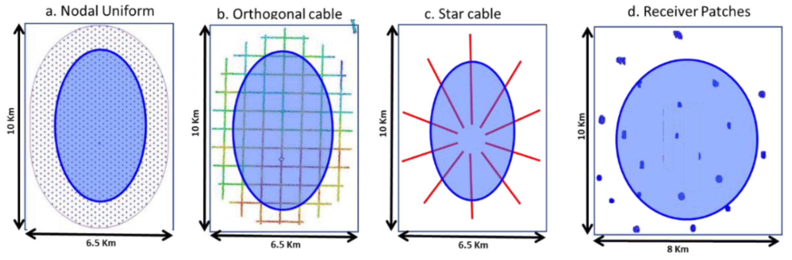
Figure 3.
Surface recording grids for fracture seismic during the monitoring of stimulations. The grid should cover the desired area around the wells being monitored plus additional area to capture the required aperture for the one-way depth migration. The ideal grid is uniform distribution of geophones as shown in (
a). The uniform layout has the minimum amount of amplitude artifacts in the fracture seismic intensity volumes. When using a cable system, the geophones are best configured in orthogonal lines (
b). The star cable layout (
c) provides good imaging in the center portion of the grid but the fracture seismic intensity volume suffers location distortions in the outer areas. The patch grid (
d) provides the lowest-quality fracture seismic intensity volumes and has very high amplitude artifacts. Figure modified from Sicking et al. (2019) [
5,
6].
Figure 4.
Buried geophone arrays are the best option if monitoring will be carried out multiple times over the same area. They are buried 30 to 100 m deep and have the advantage that they do not record the surface wave noise that is encountered on the surface arrays, so the density of geophones is reduced. Surface arrays require 30 to 60 geophones per square kilometer while buried geophone arrays require only 1 to 3 per square km. The geophones can be monitored for each new project by hooking up recorders to each geophone for the time of the project. The figure to the left is a map of the fractures extracted from the survey. Figure modified from Sicking et al. (2019) [
5,
6].
Figure 5.
Passive seismic recorded using the geophones layout for the 3D reflection seismic recording. The receiver grid is rolled with the 3D acquisition and every few days the active sources are shut down for a few hours while the geophone outputs are recorded in continuous mode. In this example, the area of interest (blue) is recorded in seven separate recording times on different days. The seven fracture seismic intensity volumes have 50% overlap and are merged after the seven final intensity volumes are computed. Merging seven independently recorded and processed volumes causes artifacts at the seams. The fracture seismic intensity volume is discussed in
Section 3.5.
Figure 6.
The patch receiver layout is designed such that there are 15 to 25 patches and within each patch there are 50 to 200 geophones. This layout allows for the suppression of surface wave noise within each patch and is focused on detecting and locating MEQs. For computing fracture seismic intensity volumes using one-way depth migration, this design is inferior. The geophone layout is shown on the left. A synthetic trace was computed for each geophone that would provide a uniform amplitude in the output fracture seismic intensity volume if a uniform grid was using the recording. When the synthetic is input to the one-way depth migration using geophone locations only at those for the patch geometry, the depth slice shown on the right is produced. The slice is for the area in the red box on the left. The patch geometry causes the short and long wavelength amplitude artifacts, and these will overprint any fracture patterns that may be imaged.
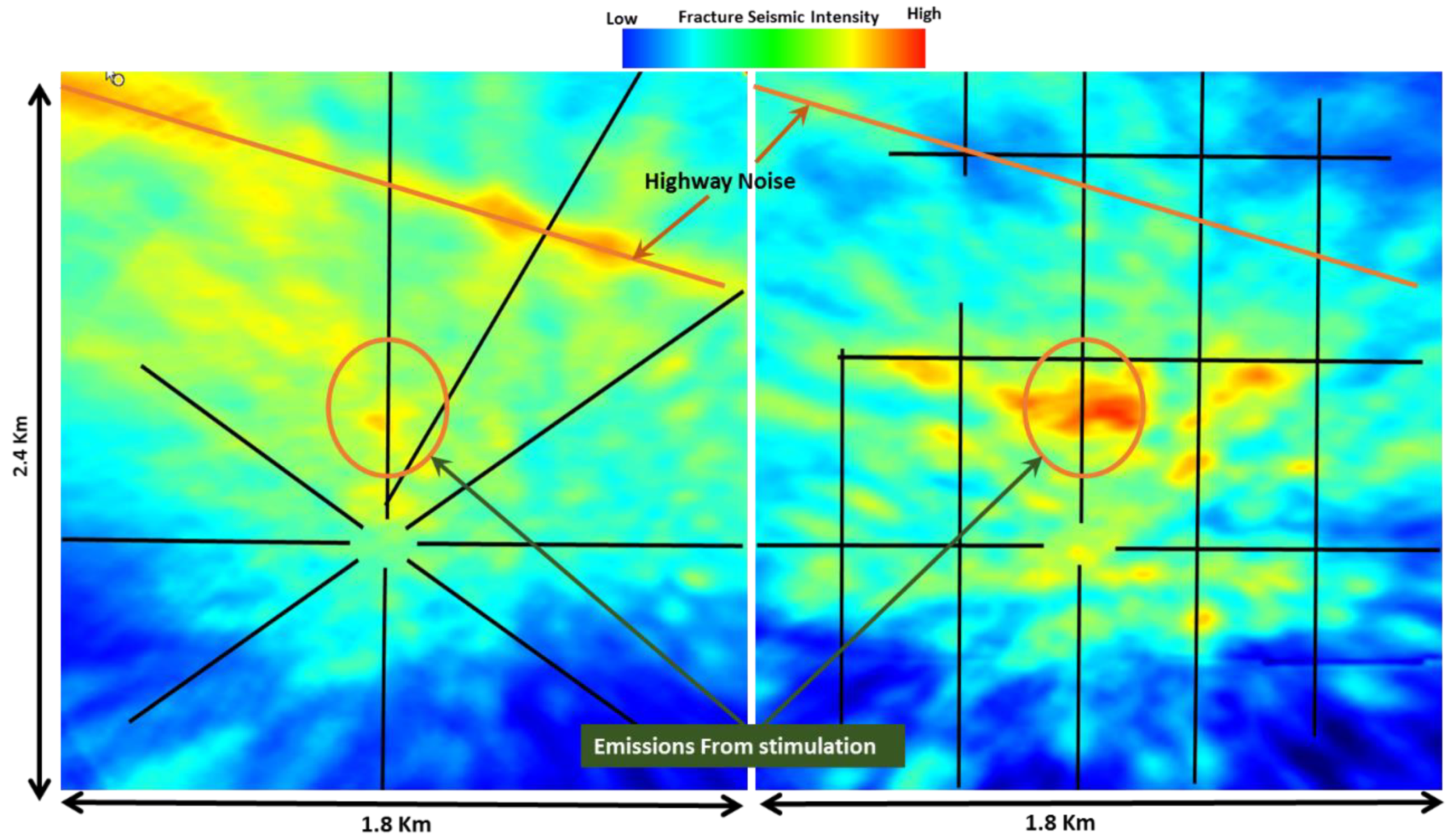
Figure 7.
Highway noise in the star grid versus orthogonal grid. All data were recorded simultaneously so the signal content is the same for the star grid and the orthogonal grid. The star grid does not cancel the horizonal noise perpendicular to the star arm. The orthogonal grid suppresses the highway noise and the signal from the stimulation is enhanced.
Figure 8.
Continuous but erratic signals along the stationary source-receiver path can overwhelm fracture seismic signals. The left panel shows the locations for the receivers, the well head, and compressor noise sources. The right panel shows the ray paths from the well head to a single receiver for various types of seismic waves. The noise is generated at all times and the ray paths are fixed so the wave forms on the receiver trace are very repetitive. (Figure from Sicking et al., 2016) [
21].
Figure 9.
The cepstral filtering process to remove stationary noise. The stationary noise becomes spikes in the spectral domain (
top panel). In the cepstral domain, these spikes are spread across all quefrencies (
middle panel). The fracture seismic signals are in the lowest 2% of the quefrencies. After the application of the low pass filter in quefrency, the inverse transform to the spectral domain is shown in the bottom panel. (Figure from Sicking et al., 2016) [
21].
Figure 10.
Cepstral filtering reveals the presence of a small microearthquake in these multichannel fracture seismic data. The top panel shows the traces as recorded in the field. The middle panel show that traces after cepstral filtering revealing the microearthquakes (MEQ). The bottom panel shows the trace data after all filtering has been applied. Figure from Sicking et al. (2016) [
21].
Figure 11.
Surface noise in the traces appears in the spectrogram as narrow frequency band noise (top panel). The time window indicated by the red bars was used to compute a depth slice and a vertical slice of the fracture seismic intensity volume (bottom two panels). The narrow frequency band noise shown in the spectrogram causes the linear features in the fracture seismic intensity volume noted by the black lines. Tracking the black lines back to the intersections reveals the surface location of the noise source.
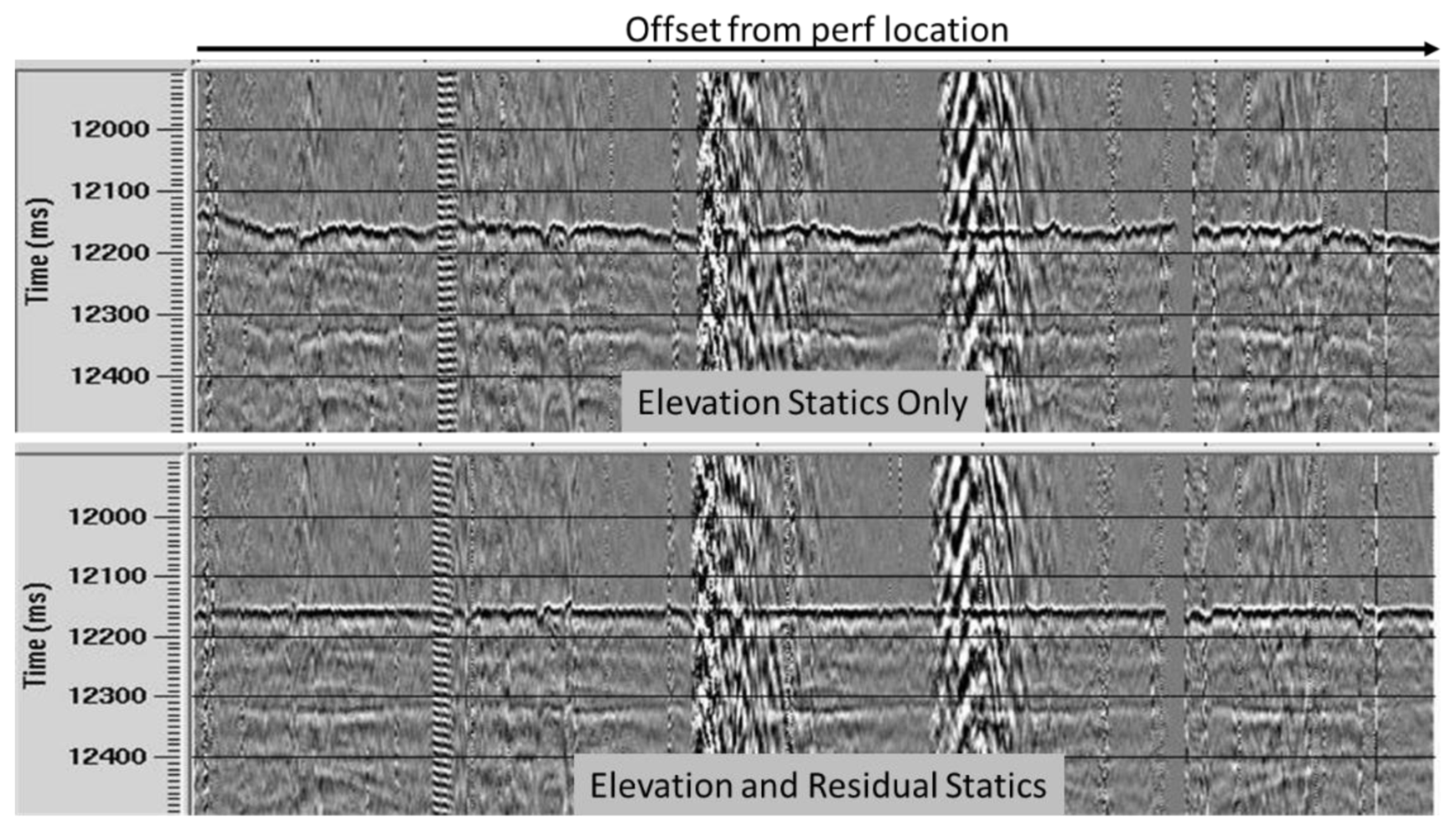
Figure 12.
The top panel shows the traces sorted by offset from the X, Y location of the perf shot and with the time shifts applied using travel times from the perf location in depth to each receiver such that they should all be flattened at the same time. The traces are adjusted for elevation differences between the traces. The bottom panel shows the traces time shifted for the residual differences remaining on the traces in the top panel.
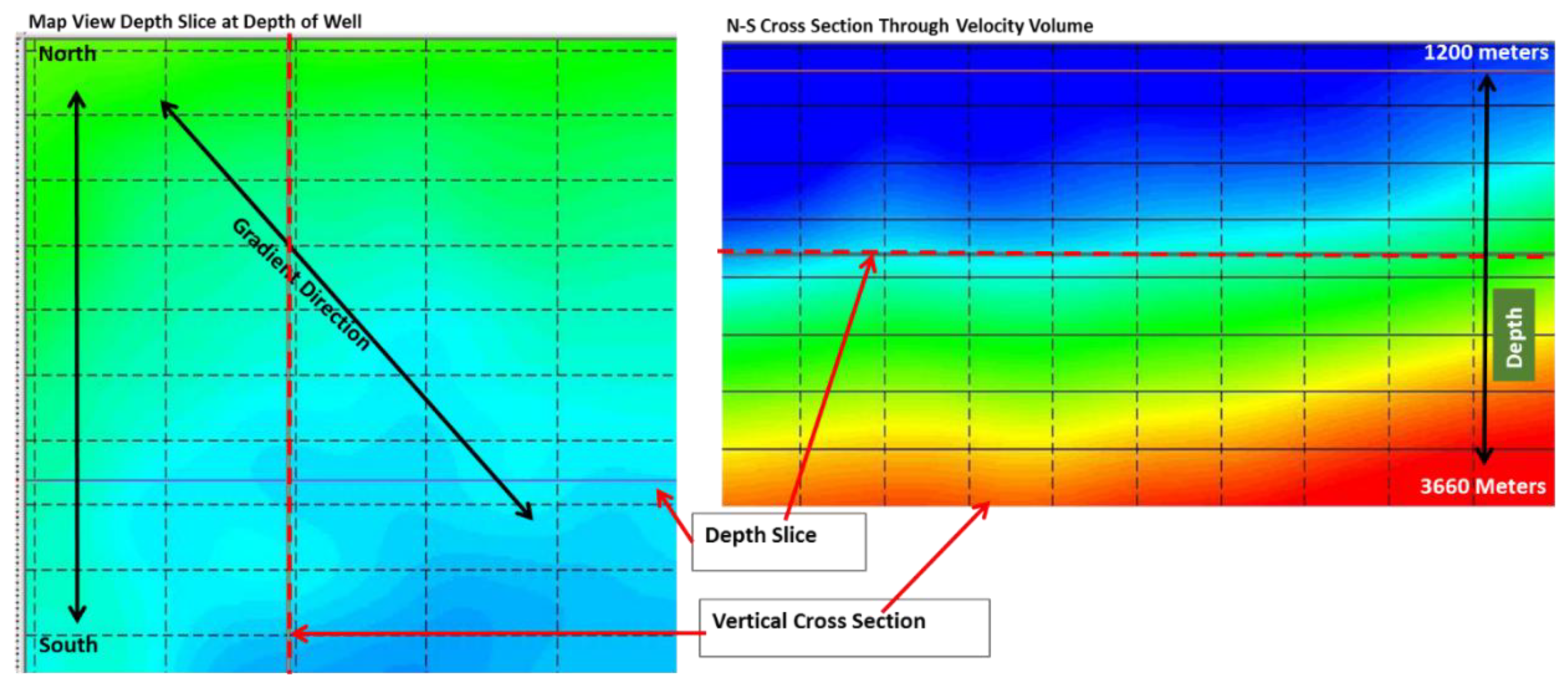
Figure 13.
The velocity volume computed from the 3D reflection seismic shows a gradient. Using the 1D velocity model derived from the sonic log and this gradient, the perf shots can be positioned to match the known locations. Using this method to calibrate the location accuracy avoids the requirement to build a 3D interval velocity model.
Figure 14.
3D complex velocity model in thrust zone computed using iterative depth migration. The fracture seismic intensity volumes computed with this velocity model will tie the reflection data and the fracture seismic intensity can be mapped onto the geologic structures.
Figure 14.
3D complex velocity model in thrust zone computed using iterative depth migration. The fracture seismic intensity volumes computed with this velocity model will tie the reflection data and the fracture seismic intensity can be mapped onto the geologic structures.
Figure 15.
Resonance during stimulation. Eagle Ford during the startup of the stimulation for Stage 1. The resonances show a transition from dispersive to turbulent flow. There is a very pronounced change at the time when the formation breaks down.
Figure 15.
Resonance during stimulation. Eagle Ford during the startup of the stimulation for Stage 1. The resonances show a transition from dispersive to turbulent flow. There is a very pronounced change at the time when the formation breaks down.
Figure 16.
The spectrogram for 13 min of trace data recorded in the New Albany shale during stimulation correlates with the pressure and slurry rate curves. The pressure and slurry rate curves are shown in the top panel and the spectrogram is shown in the bottom panel. Four different time windows are denoted by the yellow lines and show that the changes in the treatment curves are correlated with changes in the spectrogram.
Figure 17.
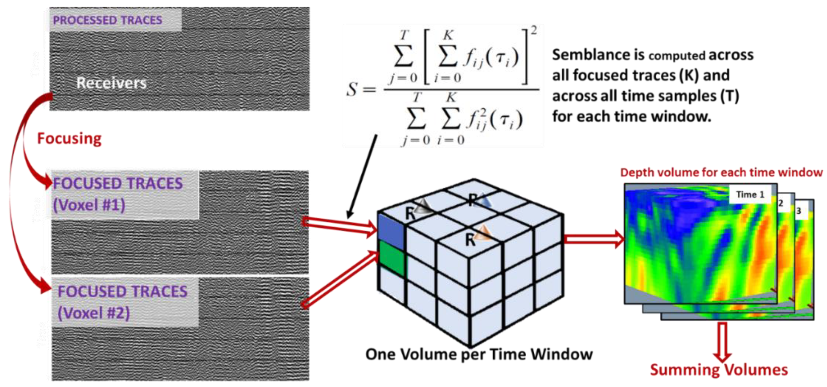
Workflow for one-way travel time depth migration. After trace processing and velocity model building and calibration, the traces are depth migrated for each time window and each depth voxel for the time interval that will be summed; fij is the trace amplitude at trace I and time j.
Figure 17.
Workflow for one-way travel time depth migration. After trace processing and velocity model building and calibration, the traces are depth migrated for each time window and each depth voxel for the time interval that will be summed; fij is the trace amplitude at trace I and time j.
Figure 18.
Integration of fracture seismic volumes increases the location accuracy, the S/N, and the resolution. For 10 s of integration, the fault is not visible. After 1 min of integration, the fault begins to be recognized. After 5 min, the fault is well defined and after 15 min, it is well resolved.
Figure 19.
Comparison of the fracture image from fracture seismic traces and the distributed acoustic sensing (DAS) log from a fiber system recorded during the stimulation. The DAS plots and the fracture image show the same result, which supports the interpretation that the location accuracy of fracture imaging is on the order of 8 m.
Figure 20.
Comparison of fracture images from fracture seismic to the MEQ locations in the same data. The fracture seismic data were recorded using a buried array in the Eagle Ford. There is only a partial correlation between the fracture surfaces and the MEQ.
Figure 20.
Comparison of fracture images from fracture seismic to the MEQ locations in the same data. The fracture seismic data were recorded using a buried array in the Eagle Ford. There is only a partial correlation between the fracture surfaces and the MEQ.
Figure 21.
Fracture seismic imaging of the subsurface is applied before, during, and after hydraulic stimulation.
Figure 21.
Fracture seismic imaging of the subsurface is applied before, during, and after hydraulic stimulation.
Figure 22.
Intensity bursts during stimulation. A burst of higher amplitude waveforms in the trace data continued for 7 s. The spectrogram of the 7 s is shown on the left. The amplitude of the signals was sufficiently high that the waveforms are clearly visible in the individual traces as shown in the plot on the right.
Figure 23.
Computing an integrated fracture seismic intensity volume over the 7 s of data in
Figure 22 and plotting on the reflection seismic shows that the energy came from a fracture in a small syncline that extends in depth from the Buda to the Austin Chalk and is focused into a very small area just to the West of the well near the stage being stimulated.
Figure 24.
MEQ in the trust fault that is 300 m below the well were activated during only four middle stages of the well treatment. The pressure from the stimulation propagated along the tear fault down to the thrust and caused activation in the thrust zone. The pressure from the stimulation activated resonances in the tear fault so that it was mapped in the fracture seismic intensity volume. The side view of the fracture image volume (left panel) shows the tear fault, the well, and the MEQ in the trust fault. The oblique view (right panel) show that the tear fault is very close to the well (50 m).
Figure 25.
Identifying zones of fracturing in reservoir before drilling. Panel (a) shows the fracture seismic intensity extracted from the volume along the reservoir horizon with the overlay of the structural contours interpreted from the 3D reflection seismic. The traces of the thrust faults are shown. The highest fracture seismic are parallel to and out in front of the thrust fault. Panel (b) shows a vertical cross section through well X with the fracture seismic overlaid on the reflection seismic. The yellow line shows the horizon that was extracted to get the slice shown in (a). The fracture seismic intensity is higher down dip from where well X was drilled. Dry holes (small black circles) drilled before this analysis are in zones of low fracture seismic intensity. An old well that blew out (shown by the small red circle) and Well X are in zones of high fracture seismic.
Figure 26.
Slices of the fracture seismic intensity volume that was computed from data recorded during a 3D reflections seismic acquisition before the well was drilled. The depth slice (a) of the fracture seismic intensity volume is shown at the depth of the proposed well. The vertical slice (b) is along the path of the proposed well. The logs of the acid uptake show that the uptake was highest in the zones of highest fracture seismic intensity and lowest in the zones of low fracture seismic intensity. This result supports the interpretation that the fracture seismic intensity shows the zones of natural fractures.
Figure 27.
Depth slice of the fracture seismic intensity volume that was computed from fracture seismic recorded during a 3D reflections seismic acquisition before the well was drilled. The seams in the final volume are the result of merging the seven independent volumes. The linear feature that runs East to West in the North of the Volume is also seen in the 3D reflection volume.
Figure 28.
Spectrograms computed from pre-stimulation fracture seismic data (top) and data recorded during stimulation (bottom).
Figure 28.
Spectrograms computed from pre-stimulation fracture seismic data (top) and data recorded during stimulation (bottom).
Figure 29.
The fracture seismic intensity volume computed from fracture seismic data recorded before stimulation show that the stimulation activated the same fractures that were mapped before the stimulation activity. The left panel shows a depth slice of the intensity volume from the pre-stimulation data. The middle panel shows the depth slice of the pre-stimulation intensity with the overlay of the fractures active during stimulation. The right panel shows the connectivity pathways computed from the 16 intensity volumes computed for each stage.
Figure 30.
Spectrogram during Stage 1 startup shows the resonances transition from low amplitude to high amplitude as the pressure is increased with pumping time. Formation breakdown causes a substantial change in the resonance as the fluid begins to flow into the formation. The lavender bars mark the 5 min of data that are used to compute the fracture images.
Figure 31.
Depth slice of fracture intensity volume computed for 5 min fracture seismic data and the overlay of the computed fractures. The fractures show the connectivity pathways that connect to the well at the Stage 1 perforations.
Figure 31.
Depth slice of fracture intensity volume computed for 5 min fracture seismic data and the overlay of the computed fractures. The fractures show the connectivity pathways that connect to the well at the Stage 1 perforations.
Figure 32.
Fracture images computed during stimulation for the stages of a well in the Permian showing the that the stimulated fractures open perpendicular to the well and then turn parallel to the well.
Figure 32.
Fracture images computed during stimulation for the stages of a well in the Permian showing the that the stimulated fractures open perpendicular to the well and then turn parallel to the well.
Figure 33.
Predicting pressure interferences on an adjacent well. The fracture intensity computed before the stimulation of Well B but while Well A was producing show the fractures crossing the path of Well B. The locations shown by the circles mark the stage locations along Well B that were being stimulated when pressure interferences were measured at the well head of Well A.
Figure 34.
Producing rock volume around Well A before (
left) and after (
right) the stimulation of Well B. The pressure changes in Well A (
Figure 33) during the stimulation of Well B caused production declines and also reduction in the producing volume.
Figure 34.
Producing rock volume around Well A before (
left) and after (
right) the stimulation of Well B. The pressure changes in Well A (
Figure 33) during the stimulation of Well B caused production declines and also reduction in the producing volume.
Figure 35.
Fracture seismic intensity signals decline over three years. Left: Fracture seismic intensity volumes showing the rock volume activated during stimulation, the rock volume that is active after two years of production, and the rock volume that is active after three years of production. Right: Production curves recorded at the well head showing the fluids produced over time. The passive data for year three were recorded at a time when the production curves show the well was not in production.
Figure 36.
Forecasting production before the well is drilled. Left side: Pre-drill, fracture seismic intensity-based forecast of the producing rock volume around the well. Center: Fracture seismic-based measurement of the producing volume after 2.5 years of production. Right: Overlay of the forecast and the observed producing rock volumes.


