Antarctic Sea Ice Proxies from Marine and Ice Core Archives Suitable for Reconstructing Sea Ice over the Past 2000 Years

Abstract

Dramatic changes in sea ice have been observed in both poles in recent decades. However, the observational period for sea ice is short, and the climate models tasked with predicting future change in sea ice struggle to capture the current Antarctic trends. Paleoclimate archives, from marine sedimentary records and coastal Antarctic ice cores, provide a means of understanding sea ice variability and its drivers over decadal to centennial timescales. In this study, we collate published records of Antarctic sea ice over the past 2000 years (2 ka). We evaluate the current proxies and explore the potential of combining marine and ice core records to produce multi-archive reconstructions. Despite identifying 92 sea ice reconstructions, the spatial and temporal resolution is only sufficient to reconstruct circum-Antarctic sea ice during the 20th century, not the full 2 ka. Our synthesis reveals a 90 year trend of increasing sea ice in the Ross Sea and declining sea ice in the Bellingshausen, comparable with observed trends since 1979. Reconstructions in the Weddell Sea, the Western Pacific and the Indian Ocean reveal small negative trends in sea ice during the 20th century (1900–1990), in contrast to the observed sea ice expansion in these regions since 1979.

1. Introduction

Sea ice plays a major role in modulating regional and global climate. It governs the amount of heat and sunlight absorbed by the earth’s albedo effect and the ocean-atmosphere transfer of gas and energy. Sea ice also influences biogeochemical cycling, water mass formation, ocean circulation, precipitation and atmospheric circulation [1,2]. It is a potential major source of dimethylsulphide (DMS) [3] (a climate-cooling gas), and is thought to modulate the physical and biological processes that can draw down atmospheric CO₂ into the ocean [4].

Sea ice is currently undergoing major changes. In the Arctic, sea ice has been declining rapidly over the last few decades, with an expectation of amplified global climate change due to ice-albedo feedbacks [5]. Climate models predict a rapid decline in Arctic sea ice during the 21st century, in response to anthropogenic greenhouse gas forcing, but the current rate of decline is faster than predicted [6]. Conversely, the total Antarctic sea ice cover has been steadily increasing since systematic satellite observations began in the late 1970s [7,8], although a precipitous decline since 2014 has halved the increasing trend for 1979–2018 relative to 1979–2014 [9]. At a regional scale, Antarctic sea ice trends are more variable; the Weddell Sea and the Ross Sea sectors have shown marked increases in sea ice extent [10], while the Bellingshausen Sea has seen a pronounced reduction [11]. Model simulations predict a 25% decline with little regional heterogeneity [12], partly due to underestimation of the intensification and position of the Southern Hemisphere westerly winds [13] and associated Ekman pumping of subsurface warm waters [14], as, for instance, recently illustrated in the eastern Antarctic Peninsula [15].

Observations of both Antarctic and Arctic sea ice conditions are limited to the satellite era (post 1970). Thus, it is hard to assess the significance of recent trends. Climate model simulations of future warming are heavily dependent on the historical sea ice area data [16], and thus it is of global importance that we provide reliable paleo-sea ice reconstructions to ensure that the climate models tasked with predicting future changes are fully optimised.

Prior to the satellite era (post-1970) and historical records (post-1930s), the best method for reconstructing past sea ice conditions comes from paleoclimate archives. Changes in sea ice conditions have been reconstructed from the chemical or isotopic records measured in continental ice cores. Marine sediment cores drilled in the Southern Ocean (SO) capture changes in sea ice over millennial timescales, based on fossil assemblages of marine biota and their geochemical signature that are buried in the sediments. These archives have the potential to enhance our understanding of longer term variability and place the recently observed changes in an extended context. Importantly, they also have the potential to provide realistic boundary conditions required by climate models tasked with predicting future sea ice and climate change [16]. Paleoclimate records have proved to be successful in this respect for other climate proxies. For example, reconstructions of past Antarctic surface temperature [17] and surface mass balance (SMB) [18] have successfully been used to validate regional climate models [19] and reanalysis climate data [20] and global climate simulations [21]. The success of these studies is largely a result of international efforts to collate all the available records to produce regional to continental-scale composites. In the case of SMB, data assimilation has resulted in a continent wide gridded data product that can now be directly compared with model output [22].The structure of the paper is as follows

The scarcity of records from the southern hemisphere has hindered the production of similar regional or hemispheric reconstructions for sea ice. Despite recent drilling efforts, neither the marine nor ice core networks on their own provide sufficient coverage. However, combining all the available records from multiple archives might be possible, especially over shorter time periods. The aim of this work is to establish the feasibility of producing regional to continental-scale sea ice reconstructions from Antarctica over the past 2 ka.

The structure of the paper is as follows:

• In the first section, we collate the published sea ice reconstructions derived from (1) ice cores and (2) marine sediments spanning all, or part, of the past 2 ka. For each archive we review the different proxies and approaches used to reconstruct sea ice.
• We then discuss the potential for combining ice core and marine records and the obstacles which need to be overcome.

2. Results

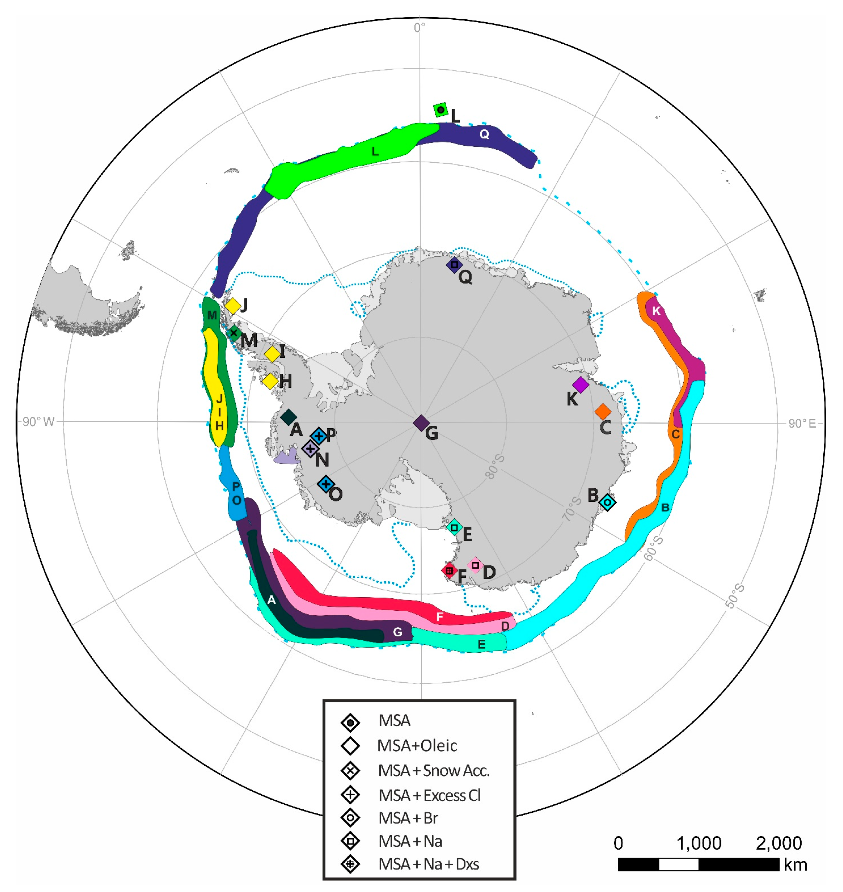
2.1. Ice Core Based Reconstructions of Sea Ice Spanning the Past 2000 Years

The poleward advection of air masses transports marine aerosols from the open ocean and the sea ice zone to the Antarctic continent. Aerosols deposited on the ice sheet, through both wet and dry deposition, are trapped in annual snow layers. Through various chemical and biological processes, the amounts of sea ice each year affects the concentrations of a number of aerosols in the atmosphere and subsequently deposited into the snow layers. Thus, the chemistry of Antarctic ice cores can be robustly used to reconstruct past sea ice conditions over centennial to millennial timescales.

There are currently only seventeen published sea ice reconstructions derived from Antarctic ice cores (

Table 1. Ice core sites with sea ice proxy records for part of the past 2 ka. MSA, Methanesulfonic acid; Br, Bromine; Na, Sodium; Dxs, Deuterium excess; ExCl, Excess Chlorine.

Map Reference	Core ID	Latitude (°)	Longitude (°)	Location	Dates	Sea Ice Proxy	Reference
A	F10	−74.57	−86.90	Ferrigno	1703–2010	MSA	[23]
B	DSS0506	−66.77	112.81	Law Dome (Summit)	1841–2012	MSA, Br	[24,25]
C	Mount Brown	−69.13	86.00	Mount Brown, Wilkes Land	1984–1999	MSA	[26]
D	TALDICE	−72.80	159.06	Talos Dome, East Antarctica		MSA, Na	[27,28]
E	NG	−77.58	162.50	Newell Glacier, Victoria Land		MSA	[29]
F	WHG	−72.90	169.83	Whitehall Glacier, Victoria Land	1883–2004	MSA, Na, Dxs	[30]
G	SP95	−90.00	0.00	South Pole	1801–1991	MSA	[31]
H	B92	−71.90	74.60	Beethoven Peninsula	1949–1991	MSA	[32]
I	DY90	−70.68	−64.87	Dyer Plateau, Antarctic Peninsula	1900–1988	MSA	[32]
J	JRI97	−64.22	−57.68	James Ross Island, Antarctic Peninsula	1832–1997	MSA	[32]
K	LGB69	−70.83	−77.07	Princess Elizabeth Land, East Antarctica	1745–1996	MSA	[33]
L	B17	−54.42	3.39	Bouvet Island, South Atlantic	2001–2017	MSA, Oleic acid	[34]
M	BP	−66.04	−64.08	Bruce Plateau, Antarctic Peninsula	1900–2009	MSA, snow accumulation	[35]
N	DIV2010	−76.77	−101.74	Thwaites Glacier, West Antarctica	1786–2010	MSA, ExCl-	[36,37]
O	THW2010	−76.95	−121.22	Thwaites Glacier, West Antarctica	1867–2010	MSA, ExCl-	[36,37]
P	PIG2010	−77.96	−95.96	Pine Island Glacier, West Antarctica	1918–2010	MSA, ExCl-	[36,37]
Q	IND-25/B5	−71.33	11.58	Central Dronning Maud Land	1905–2005	Na	[38]

). The majority of the sites are located close to the coast, in areas of high snow accumulation, and as such span only the past three centuries or less. The longest record is from the Antarctic Peninsula dating back to 1702 AD [23]).

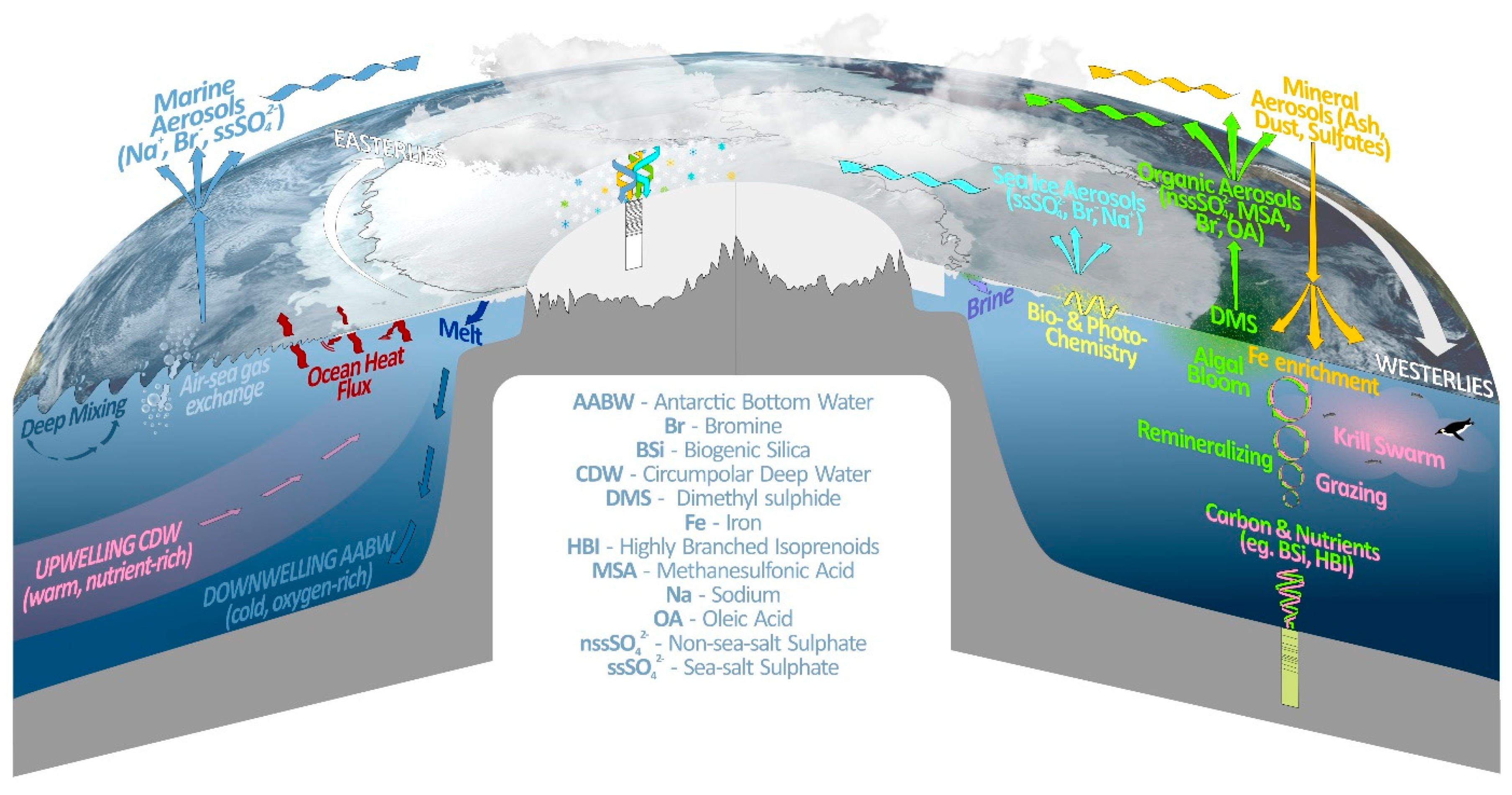
2.2. Proxies for Sea Ice

A number of chemical species have been proposed as proxies for past sea ice and will be discussed in detail in the next section. However, the concentration of all proxies in an ice core will depend on a number of important factors [39]. These include (1) conditions at the sea ice source, (2) prevailing wind direction and transport pathways, (3) deposition on route (fallout or precipitation), (4) distance from source, (5) post depositional processes in the snow (windblown ablation, melt, photo-oxidation of compounds), and (6) species migration in the firn and ice. For a proxy to be successful, changes in sea ice conditions at the source needs to be the dominant factor. Therefore, the best ice core based sea ice reconstructions originate from high accumulation coastal sites where the dominant wind direction is onshore, transporting species associated with sea ice directly to the ice core site.

In reality, the wind direction and meteorological conditions around Antarctica are highly variable. The air masses reaching an ice core site may have originated from a large area and come into contact with sea ice at several different locations. For this reason the majority of ice core-based sea ice reconstructions represent regional sea ice changes, commonly calibrated against satellite derived sea ice extent (SIE) or sea ice concentration (SIC) over a one-to-ten degree longitudinal section [23,32] (Figure 1). The range of ice core proxies for sea ice, together with the mechanisms for how they reach an ice core site, are summarized in Figure 2, together with the sea ice proxies derived from marine records.

2.2.1. Sea Salts

Over most of the Earth, sea salt aerosol originates from breaking waves over the sea surface. Once this aerosol is generated, the large particles are quickly deposited over the open water, while the smaller particles can travel long distances over the continents. Sea salt aerosol deposited on ice sheets is normally measured in ice cores as sodium (Na⁺). In Antarctica, assuming the main source of sea salt aerosol is represented by sea spray, one would expect to observe the highest sea salt concentrations during summer when the sea ice margin is closer to the continent. Aerosol chemical characterization at both coastal and inland sites in Antarctica displays a seasonal cycle of sea salt with summer minima and winter/spring maxima [40], thus excluding open water as the main source of sea salt in ice cores.

The ionic composition of sea salt aerosol arriving on polar ice sheets during winter shows a systematic depletion of the sulfate to sodium mass ratio with respect to bulk sea water [40]. For these reasons, the sea ice surface origin has been invoked by several studies [41]. During the process of sea ice formation, highly saline brine is formed on the surface of the sea ice and under particular conditions (low wind speed, temperature below −8 °C and very thin ice) frost flowers can form from these brine pockets [42,43]. For almost a decade, frost flowers have been considered the most probable phenomenon responsible of the origin of fractionated sea salt aerosol reaching coastal and inner Antarctica. However, laboratory experiments [44] showed later that frost flowers are very stable in the presence of high wind speed and no significant aerosol emission was observed. An alternative mechanism is the sublimation of salty blowing snow [45,46]. The sea ice surface can be covered by snow which may be contaminated or wetted by underlying frost flowers and brine which can be uplifted and transported by wind [47].

The potential of Na⁺ as a marker to reconstruct past sea ice changes seems to be strongly site dependent. Concentrations of Na⁺ from an array of West Antarctic ice cores revealed at positive correlation with winter SIE at some sites but not others [48]. In East Antarctica (Talos Dome), Severi et al. (2017) [28] found a good correlation between September SIE maxima and sodium flux and the same relationship is observed at Dome Fuji [49]. In both these cases, the correlations were stronger when converting sodium concentrations to fluxes, which take into account of the amount of snowfall each year. In Dronning Maud Land, the total sea salt Na+ flux was positively correlated with winter sea ice in the Weddell Sea [38]. Besides distance from open water, another factor controlling the amount of sea spray transported over the continent is wind strength, which affects the transport efficiency towards inland sites. Thus, Na⁺ has also been proposed as a proxy for marine air mass advection, suggesting that the positive correlations with sea ice may result from strengthened atmospheric circulation at the sea ice margin [50].

Several model studies have been carried out to disentangle the real relative contribution of the different sources Na⁺ (open ocean, frost flowers and blowing snow) [46,51], but more observations are needed to fully understand what can be inferred from sodium in ice core records. A promising approach to better unravel the link between sea ice and sodium flux is the comparison with marine sediment records. For example, Mezgec et al. (2017) [52] succeeded in combining complementary information measured in both terrestrial and marine records.

2.2.2. MSA

Methanesulfonic acid (MSA) is the oxidation product of dimethylsulfide (DMS), produced by marine algae. In the SO, DMS production is highest within the seasonal sea ice zone, produced primarily by phytoplankton species associated with sea ice [53]. During sea ice breakup, phytoplankton blooms release dimethylsulfoniopropionate (DMSP), which degrades to DMS by biologically-mediated processes including phytoplankton cell lysis or grazing by zooplankton [54]. The oxidation of DMS in the atmosphere also creates sulphate (SO₄²⁻), which has a number of possible sources, including sea salts and volcanic activity. However, marine biological activity is the only known source of MSA. The concentration of MSA deposited by solid precipitation onto the adjacent ice sheet is influenced by the timing, duration, and spatial extent of the sea ice breakup. Thus, the hypothesis arose that MSA preserved in ice cores could be used to reconstruct past marine productivity and seasonal sea ice cover.

MSA was one of the first organic aerosol components detected in polar ice cores [41,55]. A number of statistically significant correlations between MSA and SIE is observed at coastal sites around Antarctica [23,24,26,29,32,33]. In these studies, greater SIE during the winter months leads to a larger area of sea ice breakup during the following spring and summer, enhancing biological activity and DMS production. Thus, high MSA represents winter SIE. However, at some sites the opposing relationship is observed, with elevated MSA representing summer productivity within the sea ice zone and the presence of open water polynyas [30,36,56].

2.2.3. Halogens

Halogen species, primarily Bromine (Br⁻), have been proposed as proxies for sea ice in polar ice cores [57]. Bromine chemistry is complex, involving heterogeneous reactions of halide salts (such as HOBr and BrONO₂) in the sea ice and snow. However, studies indicate that photochemical recycling above the salt rich snow and ice surfaces drives the production of bromine in the boundary layer. The emission of Br₂ molecules, and the subsequent formation of Br-radicals, results in further heterogeneous chemical recycling known as “Bromine explosions”. Bromine explosion events occur primarily in early spring and summer [58,59].

Total bromine concentrations measured in the Talos Dome ice core, East Antarctica, revealed a depletion of bromine relative to the Br/Na ratio found in seawater during the last two glacial maximum [57]. The temporal variability of bromine in the Talos Dome record corresponded with the reconstructed sea ice duration in the Victoria Land sector derived from marine records [60]. The ratio of Br/Na has been used to calculate the bromine enrichment (Br_enr). In the Law Dome ice core, Wilkes Land, the Br_enr is correlated with first year sea ice (FYSI) in the adjacent ocean (90–110° E) and has been used to suggest a reduction in sea ice during the 20th century [25] as also observed using MSA from this site [24]. At this site, Bromine enrichment peaks during the summer, while satellite observations of BrO in the polar regions suggests an early spring peak [25,61].

The observation of large amounts of oxidized iodine in coastal Antarctica [62], from a ground-based spectrometer, suggested iodine as a possible sea ice proxy. Instrumental measurements have confirmed the flux of iodine from the sea ice to the atmosphere [63], with iodocarbon concentrations above sea ice over 10 times greater than concentration in the seawater below. Biological productivity during springtime has been suggested as the main source of iodine in the Antarctic Peninsula [64]. Excess chloride (ExCl⁻), defined as chloride in excess of the expected Cl⁻/Na⁺ ration of bulk seawater, has also been related to sea ice [36,37]. The annual cycle of ExCl⁻ exhibits a maximum in late winter, when the sea-salt aerosol is depleted in Na⁺, consistent with the timing of increased SIC around Antarctica. Total Cl⁻ and ExCl⁻ measured in a West Antarctic site (THW2010) was positively correlated with SIC in nearby polynyas [36], while winter time concentrations of ExCl⁻, measured in three West Antarctic ice cores (DIV2010, PIG2010, and THW2010), is positively correlated with winter SIC in the Bellingshausen-Amundsen Sea [37]. Future research into sea-salt ratios in ice cores would establish the possibilities of utilizing halogens (Br⁻, Cl⁻, and I⁻) as proxies for sea ice.

2.2.4. Novel Organic Compounds

Novel organic compounds in ice cores hold great promise as environmental proxies [65]. A major source of primary organic aerosol from the marine biosphere, such as fatty acids, is phytoplankton blooming events. The organic concentration of sub-micrometer aerosols is higher during biological activity in the summer [66], and studies of MSA have already shown emissions of the organic compound is related to SIC. It is therefore highly likely that concentrations of further organic compounds emitted by phytoplankton will be influenced by sea ice. Oleic acid, a short-chain unsaturated fatty acid, is a constituent of cell membranes in phytoplankton and has now been investigated in ice cores from Alaska [67], Greenland, [68], and the sub-Antarctic [34]. A positive correlation is observed between oleic acid and MSA in Alaska while King et al., (2019) [34] found a direct positive correlation between oleic acid and SIC in the region of Bouvet Island. This suggests a similar mechanism of production as MSA, whereby greater SIC in the winter results in a greater region of phytoplankton blooming along sea ice margins during spring following the break-up of sea ice. Kawamura et al. [68] instead found an inverse correlation between low molecular weight fatty acids, including oleic acid, and sea ice in the source regions of the Iceland coasts, proposing that less sea ice also indicated higher arctic temperatures, which would support greater sea-to-air transmission of marine organic matter.

In addition to MSA, a number of secondary organic aerosols (SOA) from the marine biosphere show potential for use as sea ice markers. Dicarboxylic acids (oxidation products of unsaturated fatty acids) and azelaic acid records from a Greenland ice core showed links with SICs over long time scales [67]. Oxalate, formate and acetate are oxidation products (of oxalic acid, formic acid and acetic acid respectively) that are more commonly investigated as terrestrial markers in ice cores, but do have a marine source measured in sea spray [69,70]. Only very few investigations exist for these compounds in snow and ice at remote marine locations. Legrand et al. [55] related concentrations of oxalate and formate to the presence of a local Adelie penguin populations in coastal Antarctic ice samples, while in the sub-Antarctic [34] a summertime correlation between oxalate and SIC is related to both penguin emissions and a cloud-based photo-oxidation processes.

2.2.5. Stable Water Isotopes

Stable isotope ratios of precipitation (δ¹⁸O and δD), preserved in ice cores, provide records of climate variability across a range of spatial and temporal scales. The distribution of water isotopes is dependent on temperature, thus the isotopic composition of polar ice is a powerful tool to reconstruct changes in past temperature [71,72]. Stable water isotopes fractionate due to atmospheric transport, evaporation and condensation processes. As such, changes in sea ice conditions have been proposed to influence the composition of water isotopes in coastal ice in the Antarctic Peninsula, West Antarctica and the Ross Sea region [73,74]. Observations show that during years of less extensive sea ice, greater transfer of heat and moisture inland leads to less negative δ¹⁸O values in Antarctic precipitation [75], although in West Antarctica, sea ice drives changes both in seasonal water isotopes and temperature [76]. Recently, the stable water isotope maximum observed in Antarctic ice cores during last interglacial has been reinterpreted to reflect a sea ice minimum [73,77]. Despite observations from a handful of coastal ice cores, little work has gone into validating stable water isotopes as a proxy to reconstruct past sea ice variability during recent centuries.

Nevertheless, deuterium excess has been used to reconstruct sea ice area (SIA) and, combined with MSA and Na concentrations, shows great promise as a sea ice proxy [30]. Deuterium excess, (d-excess = δD − 8 × δ¹⁸O), is a tracer of precipitation origin. It is largely controlled by the conditions at the source where moisture evaporates, in particular relative humidity and sea surface temperature (SST). These parameters control diffusive processes at the air-ocean boundary and produce a positive relationship between SST and d-excess [72]. Ice core d-excess has been used to reconstruct 20th century trends in the Ross Sea [30]. The d-excess signal in the Whitehall Glacier ice core is inversely correlated with SIA, reflecting the seasonal pattern of sea ice break out.

Water isotopes are commonly and relatively easy to measure in ice cores, yet water isotopes are only recently emerging as a potential tracer of past sea ice conditions. A large number of ice core water isotope records in Antarctica span at least the past 2 ka [17], thus ample coastal records exist to investigate d-excess as an indicator of sea ice change. However, MSA and Na concentrations were required to validate the d-excess derived SIA proxy.

2.2.6. Snow Accumulation

Another indirect proxy for sea ice in ice cores is snow accumulation. Sea ice provides a barrier between the ocean and the atmosphere and thus a reduction in sea ice can result in enhanced availability of surface level moisture and increased poleward advection of moisture transport [78]. The strong negative correlation between snow accumulation and sea ice is observed at several sites in the Antarctic Peninsula [35,75] and in a recent regional reconstruction of surface mass balance [18]. It explains the longitudinal differences in snow accumulation in the southern Antarctic Peninsula [79], which is greater at sites adjacent to the Bellingshausen Sea (where sea ice exhibits a decline) than those closer to the Amundsen Sea (where sea ice has been increasing). At Bruce Plateau, in the northern Antarctic Peninsula, a reconstruction based on annual snow accumulation reveals a 20th century decline in SIE in the Bellingshausen Sea [35]. This is in agreement with ice core reconstructions based on MSA [32] but at Bruce Plateau the relationship between SIE and snow accumulation is significantly greater than the correlations between SIE and chemical species (Na and MSA). In addition to altering moisture availability, sea ice and snow accumulation exhibit a shared response to large-scale climate variability. For example, both SIE and snow accumulation are modulated by changes in the Amundsen Sea Low, a quasi-permanent low-pressure system that drives the advection of onshore winds to the Antarctic Peninsula [79]. Thus, the lack of correlation between SIE and chemical proxies at this site suggests an indirect link between SIE and snow accumulation.

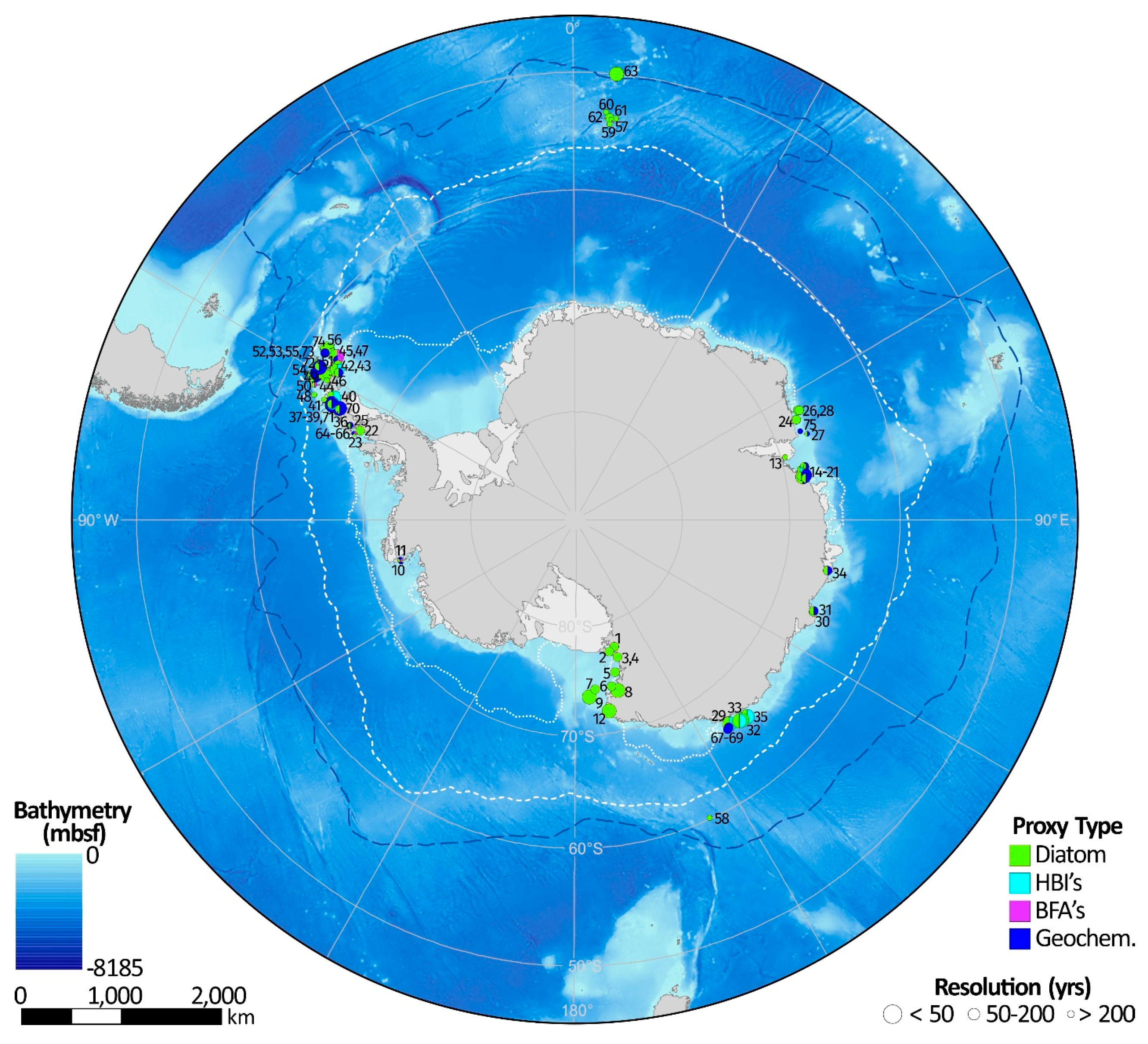
2.3. Marine Based Reconstructions of Sea Ice Spanning the Past 2000 Years

In the ocean, marine snow (comprising dead organisms, faecal matter, sand, ash, and other inorganic particles) sinks out of surface waters to the sea floor and preserves a record of past oceanic conditions in the fossils and chemical components of the accumulated marine sediment [80]. A range of different proxies can be extracted from these sediments to reconstruct past sea surface temperatures, primary productivity, ocean currents and the presence or absence of sea ice [81] (Figure 2).

Over 70 marine core sites have published sediment records containing relevant proxy data on the past 2 ka of Antarctic sea ice conditions (

Table 2. Marine core sites with sea ice proxy records for all or part of the past 2 ka.

Map Reference	Core/Site ID	Latitude (°)	Longitude (°)	Location Name	Dates **	Resolution (Lowest) $	Resolution (Highest) $	Sea Ice Proxy	Reference(s)
1	WG35	−77.989	162.853	Granite Harbor, Ross Sea	1.2 to 0.6 ka BP	60	32	Diatom	[82]
2	Multiple	−77.668	165.500	McMurdo Sound; Ross Sea	0.5 to 0 ka BP	100	56	Diatom	[83]
3	WG17	−77.000	162.850	Granite Harbor, Ross Sea	1.2 to 0.6 ka BP	60	32	Diatom	[82]
4	KC208.09	−76.972	162.876	Granite Harbor, Ross Sea	1.3 to 0 ka BP	65	33	Diatom	[82]
5	KC31	−75.700	165.418	Western Ross Sea	2.0 to 0 14C ka BP	400	222	Diatom	[84]
6	KC37	−74.499	167.744	Western Ross Sea	2.0 to 0 14C ka BP	400	222	Diatom	[84]
7	KC39	−74.474	173.474	Western Ross Sea	2.0 to 0 14C ka BP	400	222	Diatom	[84]
8	BAY05-43c	−74.000	166.050	Wood Bay, Western Ross Sea	2.0 to ~0.5 ka BP	38	15	Diatom	[52]
9	ANTA99-cJ5	−73.817	175.650	Joides Basin, Western Ross Sea	2.0 to 0 ka BP	23	9	Diatom	[52]
10	KC17	−73.420	−102.827	Ferrero Bay, Amundsen Sea Embayment	2.0 to 0 ka BP	2000	500	Diatom; BFA; Geochemistry	[52]
11	KC15	−73.360	−101.836	Ferrero Bay, Amundsen Sea Embayment	2.0 to 0 ka BP	2000	500	Diatom; BFA; Geochemistry	[52]
12	BAY05-20c	−72.300	170.050	Cape Hallet, Western Ross Sea	2.0 to ~0.1 ka BP	48	19	Diatom	[52]
13	AM02	−69.713	72.640	Amery Ice Shelf, East Antarctica	2.0 to 0.0 14C ka BP	400	222	Diatom	[85]
14	CO1011	−68.827	77.760	Flag Island Inlet, Rauer Group, Prydz Bay, EA	2.0 to 0 ka BP	2000	500	Diatom	[86]
15	CO1010	−68.817	77.833	Filla Island Inlet, Rauer Group, Prydz Bay, EA	2.0 to 0 ka BP	400	222	Diatom	[86]
16	JPC24	−68.694	76.709	Svenner Channel, Prydz Bay, EA	2.0 to 0.6 ka BP	70	36	Diatom; HBIs	[87,88,89]
17	KROCK-15-GC29	−68.664	76.696	Prydz Bay, EA	2.0 to 0 14C ka BP	400	222	Diatom	[90]
18	Abel Bay	−68.650	78.400	Abel Bay, Vestfold Hills, EA	2.0 to 0 ka BP	200	51	Diatom; Geochemistry	[91]
19	Watts Basin	−68.603	78.213	Ellis Fjord, Vestfold Hills, EA	2.0 to 0.2 14C ka BP	45	18	Diatom; Geochemistry	[92]
20	Deep Basin	−68.560	78.199	Ellis Fjord, Vestfold Hills, EA	2.0 to 0.8 14C ka BP	30	12	Diatom; Geochemistry	[92]
21	Platcha Bay	−68.515	78.478	Platcha Bay, Vestfold Hills, EA	2.0 to ~0.8 ka BP	120	63	Diatom; Geochemistry	[91]
22	JPC43	−68.257	−66.962	Neny Fjord, Marguerite Bay, AP	2.0 to 0 ka BP	100	51	Diatom	[93]
23	TPC522	−67.856	−68.205	Marguerite Bay, AP	2.0 to ~0.8 ka BP	240	133	Diatom; BFA; Geochemistry	[94]
24	KROCK-125-GC2	−67.474	64.973	Nielsen Bay, MacRobertson Shelf, EA	2.0 to 0 14C ka BP	100	133	Diatom	[95]
25	GC1	−67.180	−66.797	Lallemand Fjord, AP	2.0 to 0 14C ka BP	200	133	Diatom; Geochemistry	[96,97]
26	JPC41	−67.131	62.990	Iceberg Alley, MacRobertson Shelf, EA	2.0 to 0 ka BP	<1 *		Diatom	[98]
27	GC 5	−67.059	69.016	MacRobertson Shelf, Prydz Bay, EA	1.3 to 0 14C ka BP	700	175	Diatom; Geochemistry	[99]
28	KROCK-128-GC1	−66.983	63.154	Iceberg Alley, MacRobertson Shelf, EA	2.0 to 0.2 14C ka BP	100	51	Diatom	[95]
29	CB2010	−66.906	142.436	Commonwealth Bay, Prydz Bay	0.25 to 0 ka BP	6	3	Diatom; HBIs	[100]
30	PG1433	−66.465	110.572	Browning Bay, Windmill Islands, EA	2.0 to 0.3 ka BP	85	44	Diatom	[101]
31	PG1430	−66.453	110.498	Peterson Inlet, Windmill Islands, EA	2.0 to 0 ka BP	100; 50	51; 20	Diatom; Geochemistry	[101,102];
32	MD03-2597	−66.412	140.421	Dumont d’Urville Trough, EA	2.0 to 0.7 ka BP	<1 *		Diatom	[103]
33	DTCI2010	−66.411	140.445	Dumont d’Urville Trough, EA	0.04 to 0 ka BP	0.4	<0.4	Diatom; HBIs	[104]
34	PG1173	−66.267	100.750	Rybiy Khvost Bay, Bunger Oasis, EA	2.0 to 0 ka BP	50; 100	20; 51	Diatom; Geochemistry	[105]
35	MD03-2601	−66.052	138.557	Dumont d’Urville Trough, EA	2.0 to 1.0 ka BP	25; 50	<10; 26	Diatom; HBIs	[88,89,106,107,108,109]
36	WAP13-GC47	−65.613	−64.759	Bigo Bay, AP	2.0 to 0.1 ka BP	190	100	Diatom; Geochemistry	[110]
37	JPC10	−64.883	−64.200	Palmer Deep, AP	2.0 to 0.1 ka BP	50	20	Diatom; HBIs	[111]
38	PD92-30/178-1098A	−64.862	−64.208	Palmer Deep, AP	2.0 to 0.1 ka BP	200; 33	44; 13	Diatom; Geochemistry	[96,111,112,113]
39	178-1098B/C	−64.862	−64.208	Palmer Deep, AP	2.0 to 0.2 ka BP	100; 50; 18;	51; 20; <18	Diatom; BFA; Geochemistry	[114,115,116,117]
40	MTC18A	−64.772	−62.829	Andvord Drift, Gerlache Strait, AP	0.13 to 0 ka BP	3	1	Diatom; HBIs	[118]
41	GC 02	−64.000	−64.000	Anvers Shelf, AP	2.0 to 0.9 14C ka BP	220	122	Diatom	[119]
42	KC2B	−63.971	−57.759	Herbert Sound, James Ross Island, AP	2.0 to 0 ka BP	200; 100	105; 51	Diatom; Geochemistry	[120]
43	MTC38C; JPC38	−63.717	−57.411	Vega Drift, Prince Gustav Channel, AP	0.08 to 0 ka BP; 2.0 to 0 ka BP ***	2; 50; 20	1; 20; <20	Diatom; HBIs	[118,121]
44	PC61	−63.389	−60.319	Bransfield Strait, AP	2.0 to 0 ka BP	200	105	Diatom	[122]
45	JPC02	−63.343	−55.887	Firth of Tay, AP	2.0 to 0 ka BP	200; 50; 50	105; 20; 20	Diatom; BFA; Geochemistry	[123] [124]
46	A-3	−63.168	−59.302	Bransfield Strait, AP	1.7 to 0 ka BP	95	44	Diatom	[125,126]
47	JPC36	−63.089	−55.411	Perseverence Drift, Joinville Island, AP	0.8 to 0 ka BP; 2.0 to 0 ka BP ***	40; 20	21; <20	Diatom; BFA	[127]
48	GC 03	−63.000	−64.000	Anvers Shelf, AP	2.0 to 0.12 14C ka BP	188	99	Diatom	[119]
49	A-6	−62.912	−59.970	Bransfield Strait, AP	1.8 to 0.1 ka BP	80	41	Diatom	[125,126]
50	NCS 09	−62.594	−62.254	Outer Shelf, S. Shetland Islands	2.0 to 0 14C ka BP	400	222	Diatom; BFA	[119]
51	Gebra-2	−62.589	−58.542	Bransfield Strait, AP	2.0 to 0.2 ka BP	90	46	Diatom	[125,126]
52	1B	−62.282	−58.754	Maxwell Bay, S. Shetland Islands	2.0 to 0.1 ka BP	1900; 200	475;105	Diatom; Geochemistry	[128]
53	MC-01	−62.202	−58.727	Marian Cove, S. Shetland Islands	1.7 to 0 14C ka BP	17	<17	Diatom; Geochemistry	[129]
54	WB2	−62.200	−60.700	Outer Shelf, S. Shetland Islands	1.5 to 0 14C ka BP	38	15	Diatom; Geochemistry	[130]
55	CB2	−62.191	−58.833	Collins Harbour, Maxwell Bay, S. Shetland Islands	2.0 to 0 14C ka BP	20	<20	Diatom; Geochemistry	[131]
56	Gebra-1	−61.943	−55.170	Bransfield Strait, AP	1.6 to 0.1 ka BP	90	15	Diatom	[125,132]
57	13PC (TN057-13PC4)	−53.200	5.100	Cape Basin, South Atlantic	2.0 to 0 ka BP	20	<20	Diatom	[133]
58	E27-23	−59.618	155.238	Emerald Basin, South Indian-Pacific	2.0 to 1.5 ka BP	500	100	Diatom	[134]
59	PS1652-2	−53.664	5.100	Cape Basin, South Atlantic	2.0 to 0.6 ka BP	280	156	Diatom	[135]
60	PS1768-8	−52.593	4.476	Cape Basin, South Atlantic	2.0 to 0.8 ka BP	600	300	Diatom	[135]
61	177-1094/PS2090-1	−53.179	5.132	Cape Basin, South Atlantic	2.0 to 0.8 ka BP	240	133	Diatom	[135,136]
62	PS2102-2	−53.073	4.986	Cape Basin, South Atlantic	2.0 to 0.2 ka BP	180	95	Diatom	[135]
63	17PC (TN057-17PC1)	−50.000	6.000	Cape Basin, South Atlantic	2.0 to 4.0 ka BP	40	16	Diatom	[133]
64	KC72	−67.210	−66.888	Lallemand Fjord, AP	2.0 to 0 14C ka BP	200	105	Geochemistry	[96]
65	KC5	−67.166	−66.950	Lallemand Fjord, AP	2.0 to 0 14C ka BP	200	105	Geochemistry	[96]
66	KC75	−67.140	−66.797	Lallemand Fjord, AP	2.0 to 0 14C ka BP	200	105	Geochemistry	[96]
67	26PC12	−66.560	142.950	Mertz Ninnis Trough, EA	2.0 to 0 14C ka BP	2000	500	Geochemistry	[137]
68	17PC02	−66.540	143.200	Mertz Ninnis Trough, EA	2.0 to 0 14C ka BP	400	222	Geochemistry	[137]
69	11GC03	−66.490	143.420	Mertz Ninnis Trough, EA	2.0 to 0 14C ka BP	320	178	Geochemistry	[137]
70	WAP13-GC45	−65.752	−64.525	Bigo Bay, AP	1.2 to 0.2 ka BP	10	<10	Geochemistry	[110]
71	LMG_KC1	−64.862	−64.217	Palmer Deep, AP	0.5 to 0 ka BP	25	13	Geochemistry	[115]
72	WB1	−62.300	−60.100	Outer Shelf, S. Shetland Islands	0.8 to 0 14C ka BP	20	8	Geochemistry	[130]
73	CB1	−62.173	−58.826	Collins Harbour, Maxwell Bay, S. Shetland Islands	2.0 to 0 14C ka BP	20	<20	Geochemistry	[131]
74	A9-EB2	−61.982	−55.957	Bransfield Strait, AP	2.0 to 0 ka BP	50	20	Geochemistry	[138]
75	PS69/849-2	−67.583	68.125	Burton Basin, MacRobertson Shelf, EA	2.0 to 0.3 ka BP	850	320	Geochemistry	[139]

^$ Resolution calculated from number of samples (<5; <10; <20; <40; <100; >100) younger than 2 ka, Divided by the age interval (≤2 ka). * Laminated units of sediment. Discrete sample horizons. ** Dates are as presented in relevant publications; where more than one age model published, prioritise calendar years or (in the case of no calibrated/calendar ages) the most recent. HBI = highly branched isoprenoid; ¹⁴C ka BP = corrected ¹⁴C age; ka BP = Calendar age (Based on calibrated ¹⁴C dates, lead-210 and/or extrapolated from sedimentation rates). *** In the case of records with considerably different age ranges, both are listed in order of proxy/reference.

; Figure 3). In order to maximise the number of records considered, broad selection criteria were adopted for inclusion in this study. The records need to contain 1) at least two data points used to infer sea ice conditions during some or all of the past 2 ka or 2) adequate dating control to establish the surface/near surface age and the depth of the 2 ka interval. Many of these records extend over the Holocene or longer time intervals, with several sites affording the potential for higher resolution sampling of the past 2 ka. This results in a spatial distribution that is largely limited to the continental shelf, with only six records of adequate chronological control and/or resolution from deep ocean sites within or close to the seasonal sea ice zone.

2.4. Marine Proxies of Sea Ice

2.4.1. Diatoms

Diatoms are microscopic, unicellular algae that inhabit a wide range of aqueous to sub-aqueous environments—from boggy peat-lands through to the open ocean. Diatoms display immense morphological diversity and are renowned for the geometric patterns and intricate ornamentation of their siliceous shells (frustule). As algae, they require sunlight to photosynthesize so that in the oceans, their distribution and growth is restricted to the photic zone. Other factors limiting diatom growth include temperature, salinity and nutrient availability [140,141]. As individual species have different tolerances and preferences with respect to these controls, they occupy particular environments. It is the association between specific diatom taxa and their preferred environment that provides the basis for their use as proxies for past environmental conditions.

In the SO, diatoms offer excellent potential for reconstructing Antarctic sea ice conditions as they occupy niche assemblages close to or within the sea ice, produce intense ice edge blooms characterised by high primary- and export-production, are well-preserved in most Antarctic marine sediments and have been studied throughout the SO [142,143,144]. As a result, many studies use fossil diatoms as the basis for reconstructing past Antarctic sea ice cover.

There are two broad approaches to using fossil diatom assemblages to reconstruct past sea ice conditions: firstly, direct association of particular sea ice conditions or parameter(s) to the relative abundance(s) of sea ice-related diatom taxa and secondly, statistical methods to relate the abundance patterns of several diatom taxa or broad assemblage to a quantitative range of sea ice conditions. Both approaches make use of the ecological associations and distribution of diatoms in surface sediments (assumed to be modern) to relate to sea ice parameters (such as seasonal cover (days or months per year), seasonal or mean monthly extent (typically defined as 15% ice cover), or mean monthly SIC)) averaged over years within the satellite era to establish the proxy relationship.

The vast majority of studies that present sea ice records for the past 2 ka with adequate chronological control and resolution are from continental shelf sediments (Figure 3; Table 2) yielding a biased view of sea ice dynamics over this period. In the highly dynamic coastal environments, where other processes such as winds and mixed layer depth along with polynya presence and sea ice transport strongly impact onto diatom production and burial, statistical methods cannot be applied. There, sea ice reconstructions mainly rely on relative abundances of a few diatoms species and diatom specific organic compounds (see Section 2.4.2).

Based on sediment trap timeseries and extensive literature on SO diatom distribution, Gersonde and Zielinski (2000) [145] have shown that relative abundances >3% in Fragilariopsis curta, a diatom species thriving at very low ocean temperature and very high sea ice cover [142], both at the sea ice edge or below the ice, record the mean winter sea ice edge. This proxy has been used extensively in the Atlantic sector of the SO to reconstruct changes in winter SIE over different periods [135,136,146,147]. The approach is a little bit different in Antarctic coastal environments. As the winter sea ice edge is located far offshore (Figure 3), high relative abundances in F. curta or F. curta + F. cyclindrus (FCC) have been used to infer longer sea ice duration and greater SIC [52,85,93,94,106,107,108,111,126,132,148,149]. As such, high FCC values suggest sea ice lasting longer into the spring season and, generally, a shorter ice-free season.

In the same vein, Gersonde and Zielinski (2000) [145] proposed that relative abundances of F. obliquecostata, a sea ice related diatom [142], greater than 3% could track the mean position of the summer sea ice edge. There again, this proxy has mainly been used in offshore records from the south Atlantic to track past migrations in summer SIE [135,136,150]. In coastal environments, high occurrences of F. obliquecostata suggest sea ice presence during summer time, reflecting a minimal ice-free season.

However, the length of the ice-free season is also dependent on the timing of sea ice freezing in autumn. Thin sections of laminated sediments, preserve the depositional sequence of seasonal diatom assemblages. These studies evidenced two diatom species, Porosira glacialis and Thalasiosira antarctica, forming near mono-specific sub-micrometer laminae at the end of the summer, ice-free season. The laminae are generally composed of resting spores, the formation of which is triggered by low light levels, and attributed to mass settling events when sea ice reforms [103,148,151]. By compiling several records distributed around Antarctica, Pike et al. (2009) [89] demonstrated that P. glacialis thrives at slightly colder and icier conditions than T. antarctica and that the ratio of the two species can be used to infer the timing of sea ice formation. Ratio values above 0.1 may indicate a late sea ice melting in spring but a late sea ice freezing in autumn. However, a recent study comparing sedimentary diatom records to instrumental data off Adélie Land, East Antarctica, over the last 40 years suggested T. antarctica to be more positively correlated to early autumn sea ice return than P. glacialis [104]. It appears therefore necessary to understand the relationship between these species and autumn sea ice conditions at the regional scale before interpreting down-core records.

Diatoms can even provide information on winter SIC. Both varieties of Eucampia antarctica, namely E. antarctica var. antarctica thriving in sub-polar waters and E. antarctica var. recta living at the ice edge [142], presents the particularity to form heavily silicified winter stages that are able to germinate into short chains during winter when conditions are not too harsh [152]. These chains are composed of two pointy-horned terminal valves and a variable number of flat-horned intercalary valves. Low ratio values of terminal-to-intercalary valves indicate long chains that developed under no winter sea ice to loose winter sea ice conditions [153]. However, this proxy has not been intensively used because of generally low abundances of E. antarctica in sediment cores [154].

In offshore environments, diatom-based transfer functions are robust approaches to reconstruct both sea-surface temperatures [60,135,144,145,147] and sea ice [147,150,155,156,157] over a range of timescales. Several statistical approaches have been used, all of them having different advantages and flaws but most of the time providing similar results when applied to the same dataset [134,147,150]. Detailing the advantages and flaws of each statistical technique is beyond the scope of the present manuscript and readers are encouraged to go back to the original publications. The main issue in offshore environments is to identify sites with high accumulation rates to retrieve sediment sequences preserving the past 2 ka. Generally, high accumulation sites are located at the Polar Front in the opal belt, i.e., north of the modern winter sea ice. Only a handful of cores present sea ice records over the past 2 ka [136,157,158] indicating that SIE might have been episodically larger in the last 2000 years than today.

2.4.2. Biomarkers

Relatively new source-specific organic compounds, the C₂₅-highly branched isoprenoid (HBI) alkenes, have been developed over the last 10 years to investigate past Antarctic SIE [159,160,161,162]. Although these lipid biomarkers, composed of 25 carbon atoms, can have several structures [163], only two have currently been investigated for use in Antarctic sediments. The di-unsaturated C₂₅-HBI with a double bond, also referred to as diene, HBI II or more recently IPSO₂₅ [164] by analogy to the Artic IP₂₅ [165], is mostly sourced by the sympagic diatom species Berkeleya adeliensis [164]. This species grows as part of the sea ice diatom community, in particular in coastal zones where platelet ice is present [166]. In contrast, the tri-unsaturated C₂₅-HBIs with three double bonds, also referred to as triene or HBI III, including its two isomers Z and E, is mostly produced by the pelagic Rhizosolenia species such as R. antennata var. semispina and R. polydactyla var. polydactyla [159,160,163,167], two open ocean species that grow in regions of a retreating sea ice edge/exhibit preference for regions of retreating sea ice.

The HBIs are then transferred downward through the water column to the surface sediment probably attached to particles produced from the melting of sea ice or ice shelf, included in fecal pellets or marine snow, in a similar way than its Arctic counterpart or most of the lipid biomarkers in polar areas [168]. Although the main downward vector is still unknown within Antarctic waters, a recent study showed that the relative amount of HBIs was unchanged between the food source, ingested material and fecal pellets [169]. During this vertical transport, the effect of the visible light induced photo-degradation was invoked; however, it seems to have a little impact, especially for the less unsaturated HBI II [170]. Once in marine sediments, both HBIs II and III are relatively well preserved from significant alteration as attested by their long-term persistence in 60,000 years old marine cores [171]. However, we cannot exclude that both molecules do not undergo any degradation, especially the triene, during early diagenesis [159,172], or even later, during inappropriate storage after sediment sampling [173]. The HBIs may also be substantially affected by rapid sulfurization when conditions become anoxic in sediments [172]. It is therefore essential to detect any organic sulfur species when using any HBI records. Nevertheless, their distribution in Antarctic surface sediments is overall well consistent with modern sea ice or open water conditions [159,160,174], making this proxy reliable enough to reflect past sea ice changes.

Before interpreting the HBIs as paleoclimate indicator, it is important to fully consider the regional environmental context. Indeed, as recently underlined by Müller et al. (2009) [175,176] and Belt (2018) [162], the absence of the sea ice biomarker could reflect either permanent or sea ice free conditions, thus potentially giving an opposite interpretation of the generated records. Regional features such as glacial ice or iceberg calving could also impact sea ice presence, source-diatom growth and thereby HBI concentrations [111]. The establishment of seasonal polynyas could also affect diatom distribution and HBI production [104]. Moreover, the abundance of both sympagic and pelagic diatom species are intimately connected to numerous additional physical, chemical and biogeochemical processes (e.g., sunlight penetration, seasonal duration of sea ice, thickness of sea ice, snow accumulation, oxygen conditions, micro and macro-nutrient supply), which the source-diatom production and therefore the HBI concentration also depends on.

While extensive work still needs to be performed on this new proxy, we can circumvent most of the aforementioned issues by combining HBI records with diatom assemblages. Whilst B. adeliensis is rarely preserved in marine sediment archives due to their thin silica shells and inherent vulnerability to water column and sediment dissolution, other diatom species, associated with sea ice (e.g., Fragilariopsis curta and Fragilariopsis cylindrus) or seasonally open water/ice free conditions (e.g., Thalassiosira antarctica, Chaetoceros resting spore or Fragilariopsis kerguelensis), can be used to infer sea ice conditions [88,111,118,121]. In Antarctica, the IPSO₂₅ and IPSO₂₅/triene ratio has been utilized in eight marine cores located in the western and eastern Antarctic Peninsula [111,118,121], Prydz Bay [88] and the Adélie Basin [88,100,104], East Antarctica. Recently, a modified IPSO₂₅/triene and IPSO₂₅/brassicasterol ratio (termed PIPSO₂₅ index in reference to the Arctic PIP₂₅ index [176]) was evaluated regarding its potential use as semi-quantitative sea ice proxy [174]. Most of the existing HBI records span the Holocene (i.e, the last 11kyrs BP), of these, four cover most of the last 2000 years at decadal or sub-centennial resolution [88,111,121]. Four records from the Vega Drift and Andvord Drift in the Antarctic Peninsula, the Dumont d’Urville Trough and Prydz Bay on the East Antarctic Margin cover the last centuries [100,118] and decades [104].

2.4.3. Foraminifera

Planktic foraminifera are single-celled, marine organisms with a calcite shell. Where carbonate shells are preserved in marine sediments foraminifera provide a valuable source of proxy information, firstly, from their assemblage composition and secondly, from the geochemistry of their shells (see Section 2.4.4).

Neogloboquadrina pachyderma sinistral is the one true polar species of planktic foraminfera and typically dominates the planktic foraminifera assemblage south of the Polar Front [177] This species has also been found living within a variety of sea ice settings [178,179,180,181]. The shells of N. pachyderma sin. are rarely preserved in Antarctic sediments. However, where they are preserved, the flux and morphology of their shells within the fossil assemblage may give insights into past sea ice conditions [182]. A recent study of sediment traps on Anvers Shelf confirms that low fluxes of N. pachyderma sin., especially small, immature specimens, is consistent with sea ice cover [183]. Accordingly, high primary productivity at the sea ice margin can be associated with enhanced fluxes of large, mature specimens of N. pachyderma sin.

Benthic foraminifera, both with calcified and agglutinated tests, have species-specific environmental niches. Benthic foraminifera assemblages (BFA) can be used to infer past variables such as temperature, salinity, dissolved oxygen levels and phytodetrital flux to the sea floor. While BFA is not a direct proxy for sea ice presence, a strong presence of phytodetrius-dependant benthic foraminifera provides an indirect indicator of sea ice cover due to the control sea ice exerts over primary productivity. As such, BFA is typically used in conjunction with other proxies of past sea ice variability to ratify and support reconstructions [94,114,123,184,185,186].

2.4.4. Geochemical

Stable oxygen isotope composition (δ¹⁸O) is the most commonly used isotopic tool in paleoceanography. Within the marine realm, δ¹⁸O can be measured on calcium carbonate (foraminifera, corals, mollusc shells etc) and opal (diatoms, radiolarian). The δ¹⁸O of carbonate is controlled by temperature, sea water δ¹⁸O and a biological, or vital, fractionation effect. Since sea ice is not an optimal environment for planktic foraminifera the factors controlling oxygen isotope fractionation may become complicated and the application of δ¹⁸O to N. pachyderma sin., is not a reliable tool for inferring past sea ice conditions [183]. Furthermore, within the seasonal sea ice zone seawater δ¹⁸O and temperature typically occupy a very narrow range meaning that subtle differences within the foramiferal δ¹⁸O are easily masked by biological factors. Diatom δ¹⁸O is found to be a faithful recorder of sea water δ¹⁸O [187,188,189] however, since minimal oxygen isotope fractionation occurs during the formation and melting of sea ice [190,191] this approach is suited to documenting meteoric water fluxes rather than sea ice variability [192,193,194,195].

The δ¹³C of marine biogenic carbonate (foraminifera, corals, mollusc shells etc.) and silica (diatoms, radiolarians) is widely used to understand carbon cycling in the ocean. Primarily controlled by the isotopic composition of the dissolved carbonate in seawater, local primary productivity and remineralisation, variations in δ¹³C reflect changes in one or more of these factors. In the sea ice, preferential biological uptake of ¹²C coupled with limited sea water exchange leads to brine pockets and channels that are enriched in ¹³C. Diatoms and other algae living in these brines have δ¹³C values higher than surface waters. This more positive δ¹³C signal is particularly useful to determine whether specific diatom taxa, biomarkers and/or other organic compounds originate from within the sea ice [168,196,197]. During winter N. pachyderma sin. dwells at shallow depths, just below or within the sea ice, where scarce food supply limits energy for growth and reproduction. Specimens overwintering under these conditions appear to enter a hibernation-like state so are unlikely to incorporate a sea ice δ¹³C signal into their shells [183].

In Antarctic marine sediments, other geochemical proxies that are sensitive to primary productivity are also used as indirect indicators of sea ice, usually in conjunction with diatom or biomarker evidence. These proxies are measured on bulk sediment or diatom material and include: total organic carbon (TOC) content, biogenic silica (BSiO₂) content (weight percent), carbon/nitrogen ratios (C/N), total nitrogen percentage (TN %) and nitrogen isotopes (δ¹⁵N) [91,92,99,102,105,110,130,131,137]. The TOC and BSiO₂ content of marine sediments provide a record of export production. Whilst only a fraction of exported organic carbon is ultimately buried at the sea floor, sediment trap studies show that TOC content is proportional to export production and strongly relates to primary productivity in the surface water [198,199]. BSiO₂ is specific to organisms precipitating silica, as diatoms dominate primary productivity in the SO, BSiO₂ content provides a reliable indicator of export and primary production in Antarctic marine sediments [200,201,202,203]. Nitrogen proxies are used to resolve nutrient utilisation. In the SO, where sea-ice exerts a strong influence on primary production, gas exchange between the ocean and atmosphere, sea surface stratification and water column mixing, nitrogen proxies reflect primary productivity as well as limitations on mixing and gas exchange [91,92,94,204,205].

3. Advantages and Limitations

The relative advantages and limitations of using marine sediments and ice cores are summarized in

Table 3. Summary of the relative merits of ice cores vs. marine sediments.

Archive	Advantage	Disadvantage
Ice cores	High-resolution (seasonal to annual) Potential to provide centennial to millennial reconstructions Variety of proxies available Records provide local to regional information Possible to calibrate with satellite and observational sea ice data	Limited spatial coverage Limited to coastal regions Proxies dependent on meteorological conditions Potential post depositional changes No records yet that cover full 2000 year period
Marine sediments	Moderate resolution (annual to centennial) Potential to increase resolution of many records Variety of proxies available Proxies common in Antarctic marine sediments Records provide site specific to local information Circum-Antarctic potential	Uneven spatial coverage Resolution dependent on sedimentation rates and potentially compromised by bioturbation Proxies dependent on good preservation with minimal lateral transport Detect the relative changes in sea ice (no quantification yet). Chronological control limited by availability of dating material, and accuracy/errors of dating techniques. Inability to distinguish between persistent multi-year sea ice cover and ice-shelf setting Proxies not standardised

.

3.1. Ice Cores

The optimal location for continental ice core based sea ice reconstructions are high accumulation coastal regions, where the prevailing wind originates from or travels over the adjacent sea ice zone. Alternatively, ice-capped islands in, or on the margin of, the sea ice zone may be similarly useful. The high snow accumulation, combined with enhanced analytical capabilities, result in multiple sea ice proxies from the same ice core at annual to sub-seasonal resolution. However, a limitation of the high accumulation sites is that few coastal ice cores extend beyond a few hundred years (Figure 4).

The majority of ice core based sea ice reconstructions overlap with the satellite observations of sea ice, available from 1979 onwards, providing a direct calibration tool for ice core based proxies [23] and the possibility to run backtrajectory models to determine the source region and transport paths of proxies reaching an ice core site [206]. The development of new proxies has the potential to reconstruct sub-annual sea ice changes. For example, the MSA record reflects the changes in winter SIE, while bromide captures changes from multi-year to first-year sea ice.

However, the dependence of favourable meteorological conditions (onshore winds) is a limiting factor. Not all ice core sites will yield a reliable sea ice record and those that do rely on the assumption that the meteorological conditions have remained stable through time [11]. Even if the conditions delivering a chemical or isotopic species to an ice core site are favourable, there are a number of post depositional processes which can limit its use as a proxy. Post depositional changes include (1) wind drift or erosion, (2) reactions or transfer at the air-ice interface, (3) diffusion with depth, (4) migration across seasonal boundaries and (5) sample loss during storage.

3.2. Marine Records

Marine sea ice proxies offer the potential for excellent circum-Antarctic coverage of sea ice reconstructions at a variety of temporal resolutions (annual to centennial) over the past 2 ka. Whilst diatomaceous sediments are available throughout the continental shelf region, the existing distribution of records reflects the frequency and accessibility of logistical routes to Antarctic Bases, with the highest concentration of sites in the Northern Antarctica Peninsula and the Western Ross Sea (Figure 3). As mentioned above, the identification of high sediment accumulation rates and recovery of cores covering the past 2 ka is also a challenge in offshore environments. Figure 3 highlights how the distribution of published records biased our understanding of sea ice history over the past millennia.

The main weakness in the use of marine sea ice proxies over the past 2 ka is the lack of proxy calibration. With the exception of diatom transfer functions, most of sea ice reconstructions based on diatom abundance and HBI concentrations are inferred from ecological associations and changes relative to core top measurements. These approaches rely on the composition of core top sediments accurately reflecting the modern sea ice setting. Whilst this is a standard assumption for marine sediment proxies, declining (increasing) Antarctic sea ice distribution over recent decades may lead to proxies predisposed to underestimate (overestimate) past sea ice, as observed in a pilot study to calibrate the HBI IPSO25 vs. satellite-derived winter SIC in the Antarctic Peninsula [174]. The diversity of sea ice proxies used to infer sea ice conditions can also be considered a weakness, making comparison of sea ice histories problematic and deterring regional assimilations. The diversity of the sea ice proxies, each recording a different aspect of sea ice conditions, may also provide a more exhaustive view of past sea ice changes once proxies are better understood.

Other limitations that are not specific to sea ice reconstructions but common to all Antarctic marine sediment archives include: dating uncertainty (i.e., variable reservoir age and local contamination offset) [207,208,209,210] and depositional modification (i.e., transport, winnowing, bioturbation and dissolution).

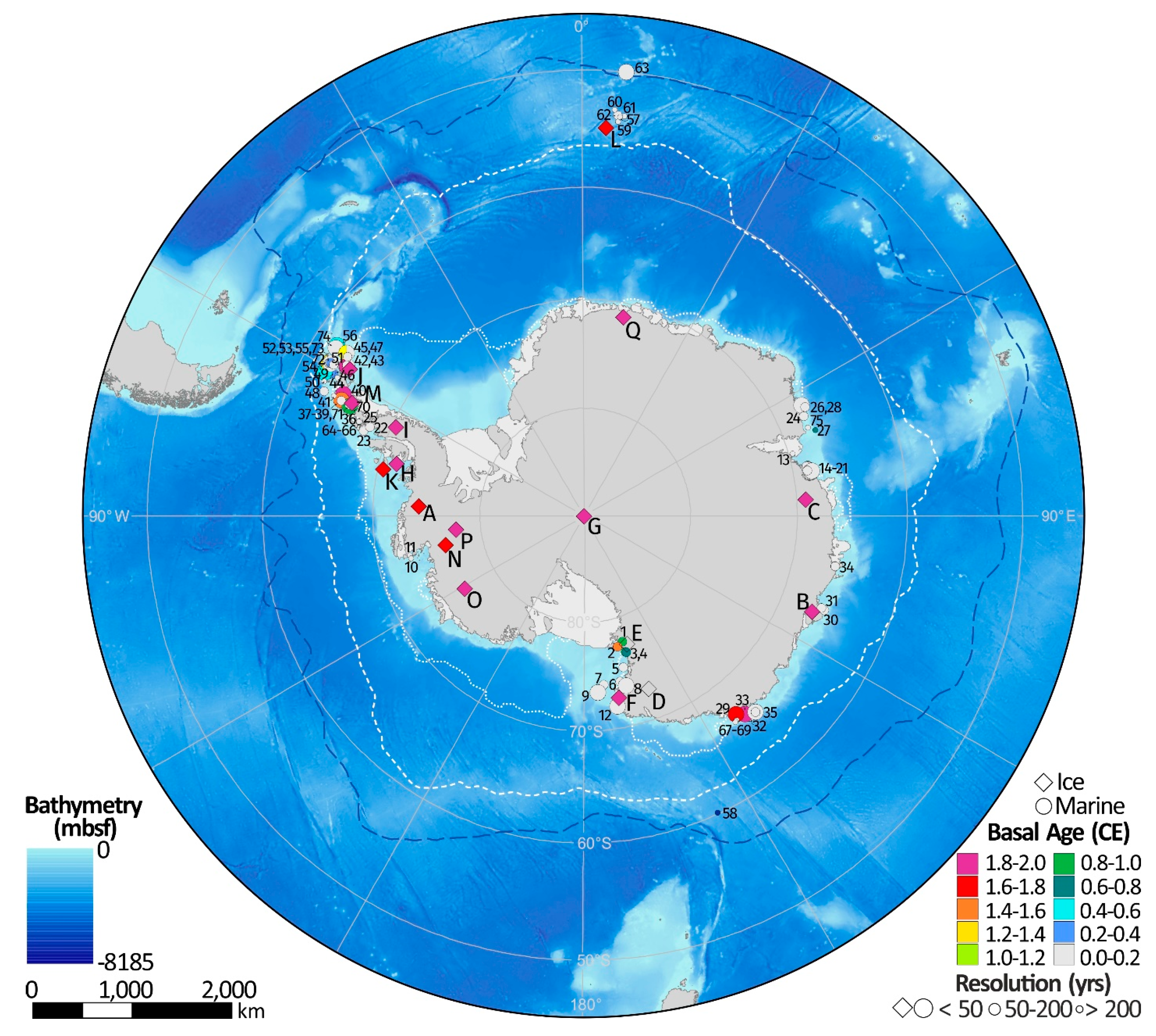
4. Feasibility of Combining Marine and Ice Core Records over the Past 2000 Years

The target period for this study is sea ice reconstructions that span, or partially span, the past 2 ka. A total of 92 sites exist with published records of sea ice variability during this time period, 75 marine sites and 17 ice cores (Table 1 and Table 2).

4.1. Spatial Coverage

The spatial distribution of sea ice reconstructions is limited (Figure 4). However, the current distribution of records is favourable for reconstructing changes in the Bellingshausen Sea and the Ross Sea, two regions that have been experiencing considerable change during the observational period. The greatest data density is around the Antarctic Peninsula, especially in the north, where multiple marine and ice core records have been used to reconstruct sea ice over the past 2 ka. The second highest data density is the Ross Sea region while there is a notable absence of records from the South Atlantic sector. No ice core records exist from the Weddell Sea coast or Dronning Maud Land. A few marine records exist in the deep ocean however the majority of these sites do not contain data relating to sea ice changes over the past 2 ka.

Combining both the marine and ice core records does increase the spatial coverage; however, at present we do not have enough records to produce a circum-Antarctic sea ice reconstruction. More data is urgently needed in the South Atlantic sector and beyond the continental shelf.

4.2. Temporal Coverage

The ice core records are all available at annual resolution or higher, while the marine records are mainly in the multi-decadal to centennial range (Figure 4). A number of the marine records span all or most of the past 2 ka, with the potential to capture decadal-to-centennial scale variability. Conversely, the longest ice core record extends just 300 years, which is arguably too short a time period to investigate the full range of natural variability.

However, within the network of records a few sites do show promise for a cross comparison between marine and ice core records. In the Antarctic Peninsula, two marine records have a comparable sample resolution and age-scale to that of the ice core records. The Vega drift, on the east Antarctic Peninsula, and the Andvord Drift, on the west [118]. Both records contain diatoms and HBI records at greater than two-year resolution, spanning the time period 1918–2000 and 1875–2000 respectively. Their locations within the fjord system suggest that the marine records are strongly influenced by local, rather than regional, sea ice conditions. Nevertheless, they both exhibit a declining trend in sea ice since 1900 AD, which is comparable to the 20th century decline reconstructed from the Antarctic Peninsula ice core stack [32].

A number of other marine records may contain comparable sea ice records, however they have either not been sampled at high enough resolution over the past 2 ka or the constraints on the dating are not good enough to assign calendar ages. If resampling were possible at these sites we would greatly increase the possibilities of a multi-archive reconstruction in this region.

We also have multiple marine records in the Ross Sea, close to two ice core records, although the temporal resolution of the marine records is less favourable in this region. The highest resolution marine record is the multi-decadal record from Joides basin, western Ross Sea [52]. The resolution of between 9 and 23 years could be compared with ice core records, such as Whitehall Glacier in northern Victoria Land [30] and Talos Dome [28]. Both ice core sites capture changes in the Ross Sea during the 20th century. In the case of Talos Dome, the sea ice record is short, but the ice core extends back several thousand years, and a full 2 ka reconstruction might be possible.

A few other promising marine records exist, especially in the Dumont d’Urville basin in East Antarctica where the -CB210 site [100] and the DTCI-2010 site [104] contain either Pb²¹⁰ or a large amount of ¹⁴C dated sea ice reconstructions based on the comparison of both diatoms and HBI. The records respectively span the periods 1750–2000, 1970–2010, or the entire last 2 ka at sub-annual to decadal resolution. The location of these marine sites is currently remote from any existing ice core sites, the closest being Talos Dome, and thus future ice core drilling in this region, or the resampling of existing ice cores would be extremely valuable.

4.3. Comparable Proxies?

By reviewing the current state-of-the-art in sea ice proxies from both ice cores and marine records we have a better understanding of how the different archives may complement each other. The marine and ice core records are fundamentally reconstructing different aspects of the sea ice environment. For the ice cores, the atmospheric transport results in a reconstruction region that is distant from the ice core source. In most cases, the concentration of a chemical species has been related both physically and biologically to conditions at the sea ice edge. The absence of marine records directly below the sea ice edge makes a direct comparison difficult. Instead, the marine records are biased towards continental sites, revealing qualitative changes in seasonal duration and extent over the past 2 ka. We urgently require marine records that extend beyond the continental shelf and can capture changes at the sea ice edge, ideally beneath a region reconstructed by ice cores.

Measurements of organic compounds in ice cores offer a unique opportunity for a more direct comparison with marine archives. Oleic acid, a fatty acid found in marine diatoms, has been isolated in an ice core from Bouvet Island [34]. At this site, the oleic acid is transported by the prevailing westerly winds and thus the concentration in the ice core reflects changes in the diatom bloom which itself is driven by changes in sea ice. This would be expected to closely resemble to diatom abundance measured in marine sediments, once transport through the water column has been taken into account. Or it may be possible to directly measure oleic acid in the marine sediments. However, this new ice core proxy is still under development and has not been measured from any Antarctic locations. In addition, the comparison would also require marine sediment records from within the seasonal sea ice zone.

5. Synthesis of Sea Ice Trends during the 20th Century

The spatial and temporal resolution of published sea ice reconstructions is not sufficient to reconstruct circum-Antarctic sea ice change over the past 2 ka. However, there is sufficient data, primarily from the ice cores, to capture sea ice trends during the 20th century (Figure 5a). Eight ice core reconstructions provide quantitative estimates of sea ice extent, across almost the entire SO. The ice core reconstructions presented in Figure 5 have all been calibrated against satellite observations and provide an estimated change in sea ice extent as either a latitudinal change or an area (km²·yr⁻¹).

Only four marine records have sufficient resolution to capture changes in sea ice during the 20th century. However, as discussed previously the sea ice signal captured in coastal marine sediments may not necessarily relate to the large-scale changes in sea ice extent captured in the ice cores. In the absence of a calibrated sea ice change in the marine reconstructions, we simply indicate a sea ice increase or decrease in Figure 5. It is worth noting that the resolution of the marine cores is generally lower than the ice cores and have a greater dating uncertainty. We compare our reconstructions with the observed fast ice duration from the South Orkney Islands [211] (1903–1990) that has been calibrated against sea ice extent in the Weddell Sea (15–50° W) [23,32,211].

Multiple reconstructions reveal an increase in sea ice in the Ross Sea since 1900, advancing at a rate of approximately 2000 km² yr⁻¹. This trend is consistent with satellite observations (+5800 +/− 2900 km²·yr⁻¹ (1979–2019)) [9]. Satellite observations show that the Ross Sea has experienced the largest regional change in sea ice over the past 40 years. The ice core reconstructions demonstrate that this recent expansion in sea ice is part of a continuous 100 year trend, which has accelerated in recent decades [23].

A similar agreement between the reconstructions and the observations occurs in the Bellingshausen Sea, where sea ice extent has declined at a rate of 3700 +/− 1800 km² yr⁻¹ since 1979 [9]. This negative trend is captured in the ice core reconstructions as a decline of ~2500 km² yr⁻¹. The rate of decline is broadly consistent in both time periods, given the errors in the reconstructions and calculated sea ice extent. Coastal marine records on both the east and west of the Antarctic Peninsula also indicate reduced sea ice cover during the end of the 20th century.

Reconstructions from the Weddell Sea, the Western Pacific and the Indian Ocean indicate a small decline in sea ice extent during the 20th century (1900–1990), while the satellite observations reveal increasing trends in these regions since 1979. Based on the relatively short overlap between the reconstructions and the observations (1979–1990), we do not expect the two time-periods to show identical trends, but these differences may reflect the high level of inter-annual and inter-decadal sea ice variability in these regions.

6. Conclusions

Advances in analytical capability, together with increased drilling efforts to obtain both marine and ice core records, has greatly improved our understanding of sea ice variability over the past 2 ka. Our review of marine and ice core reconstructions highlights the increasing number of proxies for sea ice in Antarctica, with promising new research using biomarkers and organic compounds. By combining both marine and ice core reconstructions of past sea ice we could increase the spatial coverage around the southern hemisphere. However, as our study shows, despite there being almost one hundred published sea ice reconstructions from around Antarctica, spanning all or part of the past 2 ka, the spatial distribution of those records is poor. In this study we have identified the Antarctic Peninsula and the Western Ross Sea as key regions where a combined marine and ice core reconstruction of sea ice should be achievable.

With the existing marine records, there is scope for producing higher resolution records. This should be a priority in areas where we have ice core records, particularly in the Ross Sea and Antarctic Peninsula, two regions which are experiencing rapid changes during the observational period. The lowest data density is the Atlantic sector, the Weddell Sea and Droning Maud Land. Marine records do exist in the deep SO, which at first glance would be suitably located to capture changes in winter sea ice that correspond to the sea ice reconstructions captured in the ice cores. However, they either do not have sufficient sample resolution for the past 2 ka, the sedimentation rates are too low or the core top has been lost during recovery.

Despite the limited reconstructions available we do have sufficient coverage, primarily from ice cores, to reconstruct changes during the 20th century. The records from ten ice cores, and one observational record from the South Orkney islands, provides a near continuous circum-Antarctic estimate of sea ice extent from 1900 to 1990. The reconstructions demonstrate that sea ice extent in the Ross Sea has been increasing during the 20th century, while the Bellingshausen Sea has experienced a 90 year decline. This dipole pattern is reflected in the observations from 1979 to 2019 but the rate of change is accelerated during this period. Reconstructions from the Weddell Sea, the Western Pacific and the Indian Ocean reveal a small decline in sea ice extent since 1900, despite observed sea ice expansion in these regions during the satellite era (1979–2019).

References

1. Vancoppenolle, M.; Bopp, L.; Madec, G.; Dunne, J.; Ilyina, T.; Halloran, P.R.; Steiner, N. Future arctic ocean primary productivity from cmip5 simulations: Uncertain outcome, but consistent mechanisms. Glob. Biogeochem. Cycles 2013, 27, 605–619. [Google Scholar] [CrossRef] [Green Version]
2. Turner, J.; Orr, A.; Gudmundsson, G.H.; Jenkins, A.; Bingham, R.G.; Hillenbrand, C.-D.; Bracegirdle, T.J. Atmosphere-ocean-ice interactions in the amundsen sea embayment, west antarctica. Rev. Geophys. 2017, 55, 235–276. [Google Scholar] [CrossRef] [Green Version]
3. Trevena, A.J.; Jones, G.B. Dimethylsulphide and dimethylsulphoniopropionate in antarctic sea ice and their release during sea ice melting. Mar. Chem. 2006, 98, 210–222. [Google Scholar] [CrossRef]
4. Nomura, D.; Granskog, M.A.; Assmy, P.; Simizu, D.; Hashida, G. Arctic and antarctic sea ice acts as a sink for atmospheric co2 during periods of snowmelt and surface flooding. J. Geophys. Res. Ocean. 2013, 118, 6511–6524. [Google Scholar] [CrossRef] [Green Version]
5. Serreze, M.C.; Meier, W.N. The arctic’s sea ice cover: Trends, variability, predictability, and comparisons to the antarctic. Ann. N. Y. Acad. Sci. 2019, 1436, 36–53. [Google Scholar] [CrossRef]
6. Stroeve, J.; Holland, M.M.; Meier, W.; Scambos, T.; Serreze, M. Arctic sea ice decline: Faster than forecast. Geophys. Res. Lett. 2007, 34, L09501. [Google Scholar] [CrossRef]
7. Zwally, H.J.; Comiso, J.C.; Parkinson, C.L.; Cavalieri, D.J.; Gloersen, P. Variability of antarctic sea ice 1979–1998. J. Geophys. Res. Ocean. 2002, 107, 9–19. [Google Scholar] [CrossRef] [Green Version]
8. Turner, J.; Comiso, J.C.; Marshall, G.J.; Lachlan-Cope, T.A.; Bracegirdle, T.; Maksym, T.; Meredith, M.P.; Wang, Z.; Orr, A. Non-annular atmospheric circulation change induced by stratospheric ozone depletion and its role in the recent increase of antarctic sea ice extent. Geophys. Res. Lett. 2009, 36, 37524. [Google Scholar] [CrossRef] [Green Version]
9. Parkinson, C.L. A 40-y record reveals gradual antarctic sea ice increases followed by decreases at rates far exceeding the rates seen in the arctic. Proc. Natl. Acad. Sci. USA 2019, 116, 14414–14423. [Google Scholar] [CrossRef] [Green Version]
10. Parkinson, C.L.; Cavalieri, D.J. Antarctic sea ice variability and trends, 1979–2010. Cryosphere 2012, 6, 871–880. [Google Scholar] [CrossRef] [Green Version]
11. Hobbs, W.R.; Massom, R.; Stammerjohn, S.; Reid, P.; Williams, G.; Meier, W. A review of recent changes in southern ocean sea ice, their drivers and forcings. Glob. Planet. Chang. 2016, 143, 228–250. [Google Scholar] [CrossRef] [Green Version]
12. IPCC. Climate Change 2013: The Physical Science Basis. Contribution of Working Group I to The Fifth Assessment Report of the Intergovernmental Panel on Climate Change; Cambridge University Press: Cambridge, UK, 2013; p. 1535. [Google Scholar]
13. Purich, A.; Cai, W.; England, M.H.; Cowan, T. Evidence for link between modelled trends in antarctic sea ice and underestimated westerly wind changes. Nat. Commun. 2016, 7, 10409. [Google Scholar] [CrossRef] [PubMed]
14. Ferreira, D.; Marshall, J.; Bitz, C.M.; Solomon, S.; Plumb, A. Antarctic ocean and sea ice response to ozone depletion: A two-time-scale problem. J. Clim. 2015, 28, 1206–1226. [Google Scholar] [CrossRef] [Green Version]
15. Etourneau, J.; Sgubin, G.; Crosta, X.; Swingedouw, D.; Willmott, V.; Barbara, L.; Houssais, M.N.; Schouten, S.; Damste, J.S.S.; Goosse, H.; et al. Ocean temperature impact on ice shelf extent in the eastern antarctic peninsula. Nat. Commun. 2019, 10, 304. [Google Scholar] [CrossRef] [Green Version]
16. Bracegirdle, T.J.; Stephenson, D.B.; Turner, J.; Phillips, T. The importance of sea ice area biases in 21st century multimodel projections of antarctic temperature and precipitation. Geophys. Res. Lett. 2015, 42, 10832–10839. [Google Scholar] [CrossRef] [Green Version]
17. Stenni, B.; Curran, M.A.J.; Abram, N.J.; Orsi, A.; Goursaud, S.; Masson-Delmotte, V.; Neukom, R.; Goosse, H.; Divine, D.; van Ommen, T.; et al. Antarctic climate variability on regional and continental scales over the last 2000 years. Clim. Past 2017, 13, 1609–1634. [Google Scholar] [CrossRef] [Green Version]
18. Thomas, E.R.; van Wessem, J.M.; Roberts, J.; Isaksson, E.; Schlosser, E.; Fudge, T.J.; Vallelonga, P.; Medley, B.; Lenaerts, J.; Bertler, N.; et al. Regional antarctic snow accumulation over the past 1000 years. Clim. Past 2017, 13, 1491–1513. [Google Scholar] [CrossRef] [Green Version]
19. Lenaerts, J.T.M.; Fyke, J.; Medley, B. The signature of ozone depletion in recent antarctic precipitation change: A study with the community earth system model. Geophys. Res. Lett. 2018, 45, 12931–12939. [Google Scholar] [CrossRef] [Green Version]
20. Wang, Y.; Thomas, E.R.; Hou, S.; Huai, B.; Wu, S.; Sun, W.; Qi, S.; Ding, M.; Zhang, Y. Snow accumulation variability over the west antarctic ice sheet since 1900: A comparison of ice core records with era-20c reanalysis. Geophys. Res. Lett. 2017, 44, 11482–11490. [Google Scholar] [CrossRef] [Green Version]
21. Dalaiden, Q.; Goosse, H.; Klein, F.; Lenaerts, J.T.M.; Holloway, M.; Sime, L.; Thomas, E.R. Surface mass balance of the antarctic ice sheet and its link with surface temperature change in model simulations and reconstructions. Cryosphere Discuss. 2019, 2019, 1–29. [Google Scholar] [CrossRef]
22. Medley, B.; Thomas, E.R. Increased snowfall over the antarctic ice sheet mitigated twentieth-century sea-level rise. Nat. Clim. Chang. 2019, 9, 34–39. [Google Scholar] [CrossRef] [Green Version]
23. Thomas, E.R.; Abram, N.J. Ice core reconstruction of sea ice change in the amundsen-ross seas since 1702 A.D. Geophys. Res. Lett. 2016, 43, 5309–5317. [Google Scholar] [CrossRef] [Green Version]
24. Curran, M.A.J.; van Ommen, T.D.; Morgan, V.I.; Phillips, K.L.; Palmer, A.S. Ice core evidence for antarctic sea ice decline since the 1950s. Science 2003, 302, 1203–1206. [Google Scholar] [CrossRef] [PubMed]
25. Vallelonga, P.; Maffezzoli, N.; Moy, A.D.; Curran, M.A.J.; Vance, T.R.; Edwards, R.; Hughes, G.; Barker, E.; Spreen, G.; Saiz-Lopez, A.; et al. Sea-ice-related halogen enrichment at law dome, coastal east antarctica. Clim. Past 2017, 13, 171–184. [Google Scholar] [CrossRef] [Green Version]
26. Foster, A.F.M.; Curran, M.A.J.; Smith, B.T.; Van Ommen, T.D.; Morgan, V.I. Covariation of sea ice and methanesulphonic acid in wilhelm ii land, east antarctica. Ann. Glaciol. 2006, 44, 429–432. [Google Scholar] [CrossRef] [Green Version]
27. Becagli, S.; Castellano, E.; Cerri, O.; Curran, M.; Frezzotti, M.; Marino, F.; Morganti, A.; Proposito, M.; Severi, M.; Traversi, R.; et al. Methanesulphonic acid (msa) stratigraphy from a talos dome ice core as a tool in depicting sea ice changes and southern atmospheric circulation over the previous 140 years. Atmos. Environ. 2009, 43, 1051–1058. [Google Scholar] [CrossRef]
28. Severi, M.; Becagli, S.; Caiazzo, L.; Ciardini, V.; Colizza, E.; Giardi, F.; Mezgec, K.; Scarchilli, C.; Stenni, B.; Thomas, E.R.; et al. Sea salt sodium record from talos dome (east antarctica) as a potential proxy of the antarctic past sea ice extent. Chemosphere 2017, 177, 266–274. [Google Scholar] [CrossRef] [Green Version]
29. Welch, K.A.; Mayewski, P.A.; Whitlow, S.I. Methanesulfonic acid in coastal antarctic snow related to sea-ice extent. Geophys. Res. Lett. 1993, 20, 443–446. [Google Scholar] [CrossRef] [Green Version]
30. Sinclair, K.E.; Bertler, N.A.N.; Bowen, M.M.; Arrigo, K.R. Twentieth century sea-ice trends in the ross sea from a high-resolution, coastal ice-core record. Geophys. Res. Lett. 2014, 41, 3510–3516. [Google Scholar] [CrossRef]
31. Meyerson, E.A.; Mayewski, P.A.; Kreutz, K.J.; David Meeker, L.; Whitlow, S.I.; Twickler, M.S. The polar expression of enso and sea-ice variability as recorded in a south pole ice core. Ann. Glaciol. 2002, 35, 430–436. [Google Scholar] [CrossRef] [Green Version]
32. Abram, N.J.; Thomas, E.R.; McConnell, J.R.; Mulvaney, R.; Bracegirdle, T.J.; Sime, L.C.; Aristarain, A.J. Ice core evidence for a 20th century decline in sea ice in the bellingshausen sea, antarctica. J. Geophys. Res. 2010, 115, D23101. [Google Scholar] [CrossRef] [Green Version]
33. Xiao, C.; Dou, T.; Sneed, S.B.; Li, R.; Allison, I. An ice-core record of antarctic sea-ice extent in the southern indian ocean for the past 300 years. Ann. Glaciol. 2015, 56, 451–455. [Google Scholar] [CrossRef] [Green Version]
34. King, A.C.F.; Thomas, E.R.; Pedro, J.B.; Markle, B.; Potocki, M.; Jackson, S.L.; Wolff, E.; Kalberer, M. Organic compounds in a sub-antarctic ice core: A potential suite of sea ice markers. Geophys. Res. Lett. 2019, 46, 9930–9939. [Google Scholar] [CrossRef] [PubMed] [Green Version]
35. Porter, S.E.; Parkinson, C.L.; Mosley-Thompson, E. Bellingshausen sea ice extent recorded in an antarctic peninsula ice core. J. Geophys. Res. Atmos. 2016, 121, 13886–13990. [Google Scholar] [CrossRef]
36. Criscitiello, A.S.; Das, S.B.; Evans, M.J.; Frey, K.E.; Conway, H.; Joughin, I.; Medley, B.; Steig, E.J. Ice sheet record of recent sea-ice behavior and polynya variability in the amundsen sea, west antarctica. J. Geophys. Res. Ocean. 2013, 118, 118–130. [Google Scholar] [CrossRef]
37. Pasteris, D.R.; McConnell, J.R.; Das, S.B.; Criscitiello, A.S.; Evans, M.J.; Maselli, O.J.; Sigl, M.; Layman, L. Seasonally resolved ice core records from west antarctica indicate a sea ice source of sea-salt aerosol and a biomass burning source of ammonium. J. Geophys. Res. Atmos. 2014, 119, 9168–9182. [Google Scholar] [CrossRef] [Green Version]
38. Rahaman, W.; Thamban, M.; Laluraj, C. Twentieth-century sea ice variability in the weddell sea and its effect on moisture transport: Evidence from a coastal east antarctic ice core record. Holocene 2016, 26, 338–349. [Google Scholar] [CrossRef]
39. Abram, N.J.; Wolff, E.W.; Curran, M.A.J. A review of sea ice proxy information from polar ice cores. Quat. Sci. Rev. 2013, 79, 168–183. [Google Scholar] [CrossRef]
40. Wagenbach, D.; Ducroz, F.; Mulvaney, R.; Keck, L.; Minikin, A.; Legrand, M.; Hall, J.S.; Wolff, E.W. Sea-salt aerosol in coastal antarctic regions. J. Geophys. Res. Atmos. 1998, 103, 10961–10974. [Google Scholar] [CrossRef] [Green Version]
41. Wolff, E.W.; Rankin, A.M.; Röthlisberger, R. An ice core indicator of antarctic sea ice production? Geophys. Res. Lett. 2003, 30, 2158. [Google Scholar] [CrossRef]
42. Rankin, A.M.; Wolff, E.W. A year-long record of size-segregated aerosol composition at halley, antarctica. J. Geophys. Res. Atmos. 2003, 108, 4775. [Google Scholar] [CrossRef]
43. Rankin, A.M.; Wolff, E.W.; Martin, S. Frost flowers: Implications for tropospheric chemistry and ice core interpretation. J. Geophys. Res. Atmos. 2002, 107, 4683. [Google Scholar] [CrossRef]
44. Roscoe, H.K.; Brooks, B.; Jackson, A.V.; Smith, M.H.; Walker, S.J.; Obbard, R.W.; Wolff, E.W. Frost flowers in the laboratory: Growth, characteristics, aerosol, and the underlying sea ice. J. Geophys. Res. 2011, 116, D12301. [Google Scholar] [CrossRef] [Green Version]
45. Xin, Y.; John, A.P.; Richard, A.C. Sea salt aerosol production and bromine release: Role of snow on sea ice. Geophys. Res. Lett. 2008, 35. [Google Scholar] [CrossRef]
46. Jiayue, H.; Lyatt, J. Wintertime enhancements of sea salt aerosol in polar regions consistent with a sea ice source from blowing snow. Atmos. Chem. Phys. 2017, 17, 3699–3712. [Google Scholar]
47. Vega, C.P.; Isaksson, E.; Schlosser, E.; Divine, D.; Martma, T.; Mulvaney, R.; Eichler, A.; Schwikowski-Gigar, M. Variability of sea salts in ice and firn cores from fimbul ice shelf, dronning maud land, antarctica. Cryosphere 2018, 12, 1681–1697. [Google Scholar] [CrossRef] [Green Version]
48. Sneed, S.B.; Mayewski, P.A.; Dixon, D.A. An emerging technique: Multi-ice-core multi-parameter correlations with antarctic sea-ice extent. Ann. Glaciol. 2011, 52, 347–354. [Google Scholar] [CrossRef] [Green Version]
49. Iizuka, Y.; Hondoh, T.; Fujii, Y. Antarctic sea ice extent during the holocene reconstructed from inland ice core evidence. J. Geophys. Res. Atmos. 2008, 113, D15114. [Google Scholar] [CrossRef] [Green Version]
50. Mayewski, P.A.; Carleton, A.M.; Birkel, S.D.; Dixon, D.; Kurbatov, A.V.; Korotkikh, E.; McConnell, J.; Curran, M.; Cole-Dai, J.; Jiang, S.; et al. Ice core and climate reanalysis analogs to predict antarctic and southern hemisphere climate changes. Quat. Sci. Rev. 2017, 155, 50–66. [Google Scholar] [CrossRef] [Green Version]
51. Huang, J.; Jaeglé, L.; Shah, V. Using caliop to constrain blowing snow emissions of sea salt aerosols over arctic and antarctic sea ice. Atmos. Chem. Phys. 2018, 18, 16253–16269. [Google Scholar] [CrossRef] [Green Version]
52. Mezgec, K.; Stenni, B.; Crosta, X.; Masson-Delmotte, V.; Baroni, C.; Braida, M.; Ciardini, V.; Colizza, E.; Melis, R.; Salvatore, M.C.; et al. Holocene sea ice variability driven by wind and polynya efficiency in the ross sea. Nat. Commun. 2017, 8, 1334. [Google Scholar] [CrossRef] [PubMed] [Green Version]
53. Curran, M.A.J.; Jones, G.B. Dimethyl sulfide in the southern ocean: Seasonality and flux. J. Geophys. Res. Atmos. 2000, 105, 20451–20459. [Google Scholar] [CrossRef] [Green Version]
54. Dacey, J.W.H.; Wakeham, S.G. Oceanic dimethylsulfide: Production during zooplankton grazing on phytoplankton. Science 1986, 233, 1314–1316. [Google Scholar] [CrossRef] [PubMed]
55. Legrand, M.; Ducroz, F.; Wagenbach, D.; Mulvaney, R.; Hall, J. Ammonium in coastal antarctic aerosol and snow: Role of polar ocean and penguin emissions. J. Geophys. Res. Atmos. 1998, 103, 11043–11056. [Google Scholar] [CrossRef]
56. Rhodes, R.H.; Bertler, N.A.N.; Baker, J.A.; Sneed, S.B.; Oerter, H.; Arrigo, K.R. Sea ice variability and primary productivity in the ross sea, antarctica, from methylsulphonate snow record. Geophys. Res. Lett. 2009, 36, L10704. [Google Scholar] [CrossRef]
57. Spolaor, A.; Vallelonga, P.; Plane, J.M.C.; Kehrwald, N.; Gabrieli, J.; Varin, C.; Turetta, C.; Cozzi, G.; Kumar, R.; Boutron, C.; et al. Halogen species record antarctic sea ice extent over glacial–interglacial periods. Atmos. Chem. Phys. 2013, 13, 6623–6635. [Google Scholar] [CrossRef] [Green Version]
58. Impey, G.A.; Shepson, P.B.; Hastie, D.R.; Barrie, L.A.; Anlauf, K.G. Measurements of photolyzable chlorine and bromine during the polar sunrise experiment 1995. J. Geophys. Res. Atmos. 1997, 102, 16005–16010. [Google Scholar] [CrossRef] [Green Version]
59. Simpson, W.R.; Carlson, D.; Hönninger, G.; Douglas, T.A.; Sturm, M.; Perovich, D.; Platt, U. First-year sea-ice contact predicts bromine monoxide (bro) levels at barrow, alaska better than potential frost flower contact. Atmos. Chem. Phys. 2007, 7, 621–627. [Google Scholar] [CrossRef] [Green Version]
60. Crosta, X.; Sturm, A.; Armand, L.; Pichon, J.J. Late quaternary sea ice history in the indian sector of the southern ocean as recorded by diatom assemblages. Mar. Micropaleontol. 2004, 50, 209–223. [Google Scholar] [CrossRef]
61. Spolaor, A.; Vallelonga, P.; Gabrieli, J.; Martma, T.; Björkman, M.P.; Isaksson, E.; Cozzi, G.; Turetta, C.; Kjær, H.A.; Curran, M.A.J.; et al. Seasonality of halogen deposition in polar snow and ice. Atmos. Chem. Phys. 2014, 14, 9613–9622. [Google Scholar] [CrossRef]
62. Saiz-Lopez, A.; Baidar, S.; Cuevas, C.A.; Koenig, T.K.; Fernandez, R.P.; Dix, B.; Kinnison, D.E.; Lamarque, J.-F.; Rodriguez-Lloveras, X.; Campos, T.L.; et al. Injection of iodine to the stratosphere. Geophys. Res. Lett. 2015, 42, 6852–6859. [Google Scholar] [CrossRef]
63. Atkinson, H.M.; Huang, R.-J.; Chance, R.; Roscoe, H.K.; Hughes, C.; Davison, B.; Schönhardt, A.; Mahajan, A.S.; Saiz-Lopez, A.; Hoffmann, T.; et al. Iodine emissions from the sea ice of the weddell sea. Atmos. Chem. Phys. 2012, 12, 11229–11244. [Google Scholar] [CrossRef] [Green Version]
64. Granfors, A.; Ahnoff, M.; Mills, M.M.; Abrahamsson, K. Organic iodine in antarctic sea ice: A comparison between winter in the weddell sea and summer in the amundsen sea. J. Geophys. Res. Biogeosciences 2014, 119, 2276–2291. [Google Scholar] [CrossRef]
65. Giorio, C.; Kehrwald, N.; Barbante, C.; Kalberer, M.; King, A.C.F.; Thomas, E.R.; Wolff, E.W.; Zennaro, P. Prospects for reconstructing paleoenvironmental conditions from organic compounds in polar snow and ice. Quat. Sci. Rev. 2018, 183, 1–22. [Google Scholar] [CrossRef]
66. O’Dowd, C.D.; Facchini, M.C.; Cavalli, F.; Ceburnis, D.; Mircea, M.; Decesari, S.; Fuzzi, S.; Yoon, Y.J.; Putaud, J.-P. Biogenically driven organic contribution to marine aerosol. Nature 2004, 431, 676–680. [Google Scholar] [CrossRef] [PubMed]
67. Pokhrel, A.; Kawamura, K.; Seki, O.; Matoba, S.; Shiraiwa, T. Ice core profiles of saturated fatty acids (c12:0–c30:0) and oleic acid (c18:1) from southern alaska since 1734 ad: A link to climate change in the northern hemisphere. Atmos. Environ. 2015, 100, 202–209. [Google Scholar] [CrossRef]
68. Kawamura, K.; Suzuki, I.; Fujii, Y.; Watanabe, O. Ice core record of fatty acids over the past 450 years in greenland. Geophys. Res. Lett. 1996, 23, 2665–2668. [Google Scholar] [CrossRef]
69. Baboukas, E.D.; Kanakidou, M.; Mihalopoulos, N. Carboxylic acids in gas and particulate phase above the atlantic ocean. J. Geophys. Res. Atmos. 2000, 105, 14459–14471. [Google Scholar] [CrossRef]
70. Rinaldi, M.; Decesari, S.; Carbone, C.; Finessi, E.; Fuzzi, S.; Ceburnis, D.; O’Dowd, C.D.; Sciare, J.; Burrows, J.P.; Vrekoussis, M.; et al. Evidence of a natural marine source of oxalic acid and a possible link to glyoxal. J. Geophys. Res. Atmos. 2011, 116, D16204. [Google Scholar] [CrossRef] [Green Version]
71. Dansgaard, W. Stable isotopes in precipitation. Tellus 1964, 16, 436–468. [Google Scholar] [CrossRef]
72. Jouzel, J.; Lorius, C.; Petit, J.R.; Genthon, C.; Barkov, N.I.; Kotlyakov, V.M.; Petrov, V.M. Vostok ice core: A continuous isotope temperature record over the last climatic cycle (160,000 years). Nature 1987, 329, 403–408. [Google Scholar] [CrossRef]
73. Holloway, M.D.; Sime, L.C.; Singarayer, J.S.; Tindall, J.C.; Bunch, P.; Valdes, P.J. Antarctic last interglacial isotope peak in response to sea ice retreat not ice-sheet collapse. Nat. Commun. 2016, 7, 12293. [Google Scholar] [CrossRef] [PubMed] [Green Version]
74. Thomas, E.R.; Bracegirdle, T.J.; Turner, J.; Wolff, E.W. A 308 year record of climate variability in west antarctica. Geophys. Res. Lett. 2013, 40, 5492–5496. [Google Scholar] [CrossRef] [Green Version]
75. Thomas, E.R.; Bracegirdle, T.J. Precipitation pathways for five new ice core sites in ellsworth land, west antarctica. Clim. Dyn. 2015, 44, 2067–2078. [Google Scholar] [CrossRef]
76. Küttel, M.; Steig, E.J.; Ding, Q.; Monaghan, A.J.; Battisti, D.S. Seasonal climate information preserved in west antarctic ice core water isotopes: Relationships to temperature, large-scale circulation, and sea ice. Clim. Dyn. 2012, 39, 1841–1857. [Google Scholar] [CrossRef]
77. Holloway, M.D.; Sime, L.C.; Allen, C.S.; Hillenbrand, C.-D.; Bunch, P.; Wolff, E.; Valdes, P.J. The spatial structure of the 128 ka antarctic sea ice minimum. Geophys. Res. Lett. 2017, 44, 11129–11139. [Google Scholar] [CrossRef] [Green Version]
78. Tsukernik, M.; Lynch, A.H. Atmospheric meridional moisture flux over the southern ocean: A story of the amundsen sea. J. Clim. 2013, 26, 8055–8064. [Google Scholar] [CrossRef]
79. Thomas, E.R.; Hosking, J.S.; Tuckwell, R.R.; Warren, R.A.; Ludlow, E.C. Twentieth century increase in snowfall in coastal west antarctica. Geophys. Res. Lett. 2015, 42, 9387–9393. [Google Scholar] [CrossRef] [Green Version]
80. Turner, J.T. Zooplankton fecal pellets, marine snow, phytodetritus and the ocean’s biological pump. Prog. Oceanogr. 2015, 130, 205–248. [Google Scholar] [CrossRef]
81. Hillaire–Marcel, C.; Vernal, A.D. Proxies in Late Cenozoic Paleoceanography, 1st, ed.; Elsevier: Amsterdam, The Netherlands, 2007; Volume 1, p. 843. [Google Scholar]
82. Leventer, A.; Dunbar, R.B.; DeMaster, D.J. Diatom evidence for late holocene climatic events in granite harbor, antarctica. Paleoceanography 1993, 8, 373–386. [Google Scholar] [CrossRef]
83. Leventer, A.; Dunbar, R.B. Recent diatom record of mcmurdo sound, antarctica: Implications for history of sea ice extent. Paleoceanography 1988, 3, 259–274. [Google Scholar] [CrossRef]
84. Cunningham, W.L.; Leventer, A.; Andrews, J.T.; Jennings, A.E.; Licht, K. Late pleistocene-holocene marine condtions in the ross sea, antarctica: Evidence from the diatom record. Holocene 1999, 9, 129–139. [Google Scholar] [CrossRef]
85. Hemer, M.A.; Harris, P.T. Sediment core from beneath the amery ice shelf, east antarctica, suggests mid-holocene ice-shelf retreat. Geology 2003, 31, 127–130. [Google Scholar] [CrossRef]
86. Berg, S.; Wagner, B.; Cremer, H.; Leng, M.; Melles, M. Late quaternary environmental and climate history of rauer group, east antarctica. Palaeogeogr. Palaeoclimatol. Palaeoecol. 2010, 297, 201–213. [Google Scholar] [CrossRef]
87. Crosta, X.; Crespin, J.; Swingedouw, D.; Marti, O.; Masson-Delmotte, V.; Etourneau, J.; Goosse, H.; Braconnot, P.; Yam, R.; Brailovski, I.; et al. Ocean as the main driver of antarctic ice sheet retreat during the holocene. Glob. Planet. Chang. 2018, 166, 62–74. [Google Scholar] [CrossRef]
88. Denis, D.; Crosta, X.; Barbara, L.; Massé, G.; Renssen, H.; Ther, O.; Giraudeau, J. Sea ice and wind variability during the holocene in east antarctica: Insight on middle–high latitude coupling. Quat. Sci. Rev. 2010, 29, 3709–3719. [Google Scholar] [CrossRef]
89. Pike, J.; Crosta, X.; Maddison, E.J.; Stickley, C.E.; Denis, D.; Barbara, L.; Renssen, H. Observations on the relationship between the antarctic coastal diatoms thalassiosira antarctica comber and porosira glacialis (grunow) jørgensen and sea ice concentrations during the late quaternary. Mar. Micropaleontol. 2009, 73, 14–25. [Google Scholar] [CrossRef] [Green Version]
90. Taylor, F.; McMinn, A. Late quaternary diatom assemblages from prydz bay, eastern antarctica. Quat. Res. 2002, 57, 151–161. [Google Scholar] [CrossRef]
91. McMinn, A. Late holocene increase in sea ice extent in fjords of the vestfold hills, eastern antarctica. Antarct. Sci. 2000, 12, 80–88. [Google Scholar] [CrossRef]
92. McMinn, A.; Heijnis, H.; Harle, K.; McOrist, G. Late-holocene climatic change recorded in sediment cores from ellis fjord, eastern antarctica. Holocene 2001, 11, 291–300. [Google Scholar] [CrossRef]
93. Allen, C.S.; Oakes-Fretwell, L.M.; Anderson, J.B.; Hodgson, D.A. A record of holocene glacial and oceanographic variability in neny fjord, antarctic peninsula. Holocene 2010, 20, 551–564. [Google Scholar] [CrossRef]
94. Peck, V.L.; Allen, C.S.; Kender, S.; McClymont, E.L.; Hodgson, D.A. Oceanographic variability on the west antarctic peninsula during the holocene and the influence of upper circumpolar deep water. Quat. Sci. Rev. 2015, 119, 54–65. [Google Scholar] [CrossRef] [Green Version]
95. Taylor, F.; McMinn, A. Evidence from diatoms for holocene climate fluctuation along the east antarctic margin. Holocene 2001, 11, 455–466. [Google Scholar] [CrossRef]
96. Shevenell, A.E.; Domack, E.W.; Kernan, G.M. Record of holocene palaeoclimate change alond the antarctic peninsula: Evidence from glacial marine sediments, lallemand fjord. In Climatic Succession and Glacial History of the Southern Hemisphere over the Last Five Million Years; Banks, M.R., Brown, M.J., Eds.; Papers and Proceedings of the Royal Society of Tasmania; Department of Plant Science, University of Tasmania: Tasmania, Australian, 1996; Volume 130, pp. 55–64. [Google Scholar]
97. Taylor, F.; Whitehead, J.; Domack, E. Holocene paleoclimate change in the antarctic peninsula: Evidence from the diatom, sedimentary and geochemical record. Mar. Micropaleontol. 2001, 41, 25–43. [Google Scholar] [CrossRef]
98. Alley, K.; Patacca, K.; Pike, J.; Dunbar, R.; Leventer, A. Iceberg alley, east antarctic margin: Continuously laminated diatomaceous sediments from the late holocene. Mar. Micropaleontol. 2018, 140, 56–68. [Google Scholar] [CrossRef]
99. Rathburn, A.E.; Pichon, J.J.; Ayress, M.A.; DeDeckker, P. Microfossil and stable-isotope evidence for changes in late holocene palaeoproductivity and palaeoceanographic conditions in the prydz bay region of antarctica. Palaeogeogr. Palaeoclimatol. Palaeoecol. 1997, 131, 485–510. [Google Scholar] [CrossRef]
100. Campagne, P.; Crosta, X.; Houssais, M.N.; Swingedouw, D.; Schmidt, S.; Martin, A.; Devred, E.; Capo, S.; Marieu, V.; Closset, I.; et al. Glacial ice and atmospheric forcing on the mertz glacier polynya over the past 250 years. Nat. Commun. 2015, 6, 6642. [Google Scholar] [CrossRef] [Green Version]
101. Cremer, H.; Gore, D.; Melles, M.; Roberts, D. Palaeoclimatic significance of late quaternary diatom assemblages from southern windmill islands, east antarctica. Palaeogeogr. Palaeoclimatol. Palaeoecol. 2003, 195, 261–280. [Google Scholar] [CrossRef]
102. Kirkup, H.; Melles, M.; Gore, D.B. Late quaternary environment of southern windmill islands, east antarctica. Antarct. Sci. 2002, 14, 385–394. [Google Scholar] [CrossRef] [Green Version]
103. Maddison, E.J.; Pike, J.; Dunbar, R. Seasonally laminated diatom-rich sediments from dumont d’urville trough, east antarctic margin: Late-holocene neoglacial sea-ice conditions. Holocene 2012, 22, 857–875. [Google Scholar] [CrossRef]
104. Campagne, P.; Crosta, X.; Schmidt, S.; Noëlle Houssais, M.; Ther, O.; Massé, G. Sedimentary response to sea ice and atmospheric variability over the instrumental period off adélie land, east antarctica. Biogeosciences 2016, 13, 4205–4218. [Google Scholar] [CrossRef] [Green Version]
105. Kulbe, T.; Melles, M.; Verkulich, S.R.; Pushina, Z.V. East antarctic climate and environmental variability over the last 9400 years inferred from marine sediments of the bunger oasis. Arct. Antarct. Alp. Res. 2001, 33, 223–230. [Google Scholar] [CrossRef]
106. Crosta, X.; Debret, M.; Denis, D.; Courty, M.A.; Ther, O. Holocene long- and short-term climate changes off adélie land, east antarctica. Geochem. Geophys. Geosystems 2007, 8, Q11009. [Google Scholar] [CrossRef]
107. Crosta, X.; Denis, D.; Ther, O. Sea ice seasonality during the holocene, adelie land, east antarctica. Mar. Micropaleontol. 2008, 66, 222–232. [Google Scholar] [CrossRef]
108. Crosta, X.; Romero, O.; Armand, L.K.; Pichon, J.-J. The biogeography of major diatom taxa in southern ocean sediments: 2. Open ocean related species. Palaeogeogr. Palaeoclimatol. Palaeoecol. 2005, 223, 66–92. [Google Scholar] [CrossRef]
109. Denis, D.; Crosta, X.; Schmidt, S.; Carson, D.S.; Ganeshram, R.S.; Renssen, H.; Crespin, J.; Ther, O.; Billy, I.; Giraudeau, J. Holocene productivity changes off adelie land (east antarctica). Paleoceanography 2009, 24. [Google Scholar] [CrossRef] [Green Version]
110. Kim, S.; Yoo, K.-C.; Lee, J.I.; Khim, B.-K.; Bak, Y.-S.; Lee, M.K.; Lee, J.; Domack, E.W.; Christ, A.J.; Yoon, H.I. Holocene paleoceanography of bigo bay, west antarctic peninsula: Connections between surface water productivity and nutrient utilization and its implication for surface-deep water mass exchange. Quat. Sci. Rev. 2018, 192, 59–70. [Google Scholar] [CrossRef]
111. Etourneau, J.; Collins, L.G.; Willmott, V.; Kim, J.H.; Barbara, L.; Leventer, A.; Schouten, S.; Sinninghe Damsté, J.S.; Bianchini, A.; Klein, V.; et al. Holocene climate variations in the western antarctic peninsula: Evidence for sea ice extent predominantly controlled by changes in insolation and enso variability. Clim. Past 2013, 9, 1431–1446. [Google Scholar] [CrossRef] [Green Version]
112. Leventer, A. The fate of antarctic “sea-ice diatoms“ and their use as palaeoenvironmental indicators. In Antarctic Sea Ice Biological, Processes, Interactions and Variability; Union, A.G., Ed.; Volume Antarctic Research Series; American Geophysical Union: Washington, DC, USA, 1998; pp. 121–137. [Google Scholar]
113. Leventer, A.; Domack, E.W.; Ishman, S.E.; Brachfeld, S.; McClennen, C.E.; Manley, P. Productivity cycles of 200–300 years in the antarctic peninsula region: Understanding linkages among the sun, atmosphere, oceans, sea ice, and biota. Geol. Soc. Am. Bull. 1996, 108, 1626–1644. [Google Scholar] [CrossRef]
114. Ishman, S.E.; Sperling, M.R. Benthic foraminiferal record of holocene deep-water evolution in the palmer deep, western antarctic peninsula. Geology 2002, 30, 435–438. [Google Scholar] [CrossRef]
115. Shevenell, A.E.; Kennett, J.P. Antarctic holocene climate change: A benthic foraminiferal stable isotope record from palmer deep. Paleoceanography 2002, 17. [Google Scholar] [CrossRef]
116. Sjunneskog, C.; Taylor, F. Postglacial marine diatom record of the palmer deep, antarctic peninsula (odp leg 178, site 1098) 1. Total diatom abundance. Paleoceanography 2002, 17. [Google Scholar] [CrossRef]
117. Taylor, F.; Sjunneskog, C. Postglacial marine diatom record of the palmer deep, antarctic peninsula (odp leg 178, site 1098) 2. Diatom assemblages. Paleoceanography 2002, 17, PA8001. [Google Scholar] [CrossRef]
118. Barbara, L.; Crosta, X.; Schmidt, S.; Masse, G. Diatoms and biomarkers evidence for major changes in sea ice conditions prior the instrumental period in antarctic peninsula. Quat. Sci. Rev. 2013, 79, 99–110. [Google Scholar] [CrossRef]
119. Yoon, H.I.; Park, B.-K.; Kim, Y.; Kang, C.Y. Glaciomarine sedimentation and its paleoclimatic implications on the antarctic peninsula shelf over the last 15 000 years. Palaeogeogr. Palaeoclimatol. Palaeoecol. 2002, 185, 235–254. [Google Scholar] [CrossRef]
120. Minzoni, R.T.; Anderson, J.B.; Fernandez, R.; Wellner, J.S. Marine record of holocene climate, ocean, and cryosphere interactions: Herbert sound, james ross island, antarctica. Quat. Sci. Rev. 2015, 129, 239–259. [Google Scholar] [CrossRef]
121. Barbara, L.; Crosta, X.; Leventer, A.; Schmidt, S.; Etourneau, J.; Domack, E.; Masse, G. Environmental responses of the northeast antarctic peninsula to the holocene climate variability. Paleoceanography 2016, 31, 131–147. [Google Scholar] [CrossRef] [Green Version]
122. Heroy, D.C.; Sjunneskog, C.; Anderson, J.B. Holocene climate change in the bransfield basin, antarctic peninsula: Evidence from sediment and diatom analysis. Antarct. Sci. 2008, 20, 69–87. [Google Scholar] [CrossRef]
123. Majewski, W.; Anderson, J.B. Holocene foraminiferal assemblages from firth of tay, antarctic peninsula: Paleoclimate implications. Mar. Micropaleontol. 2009, 73, 135–147. [Google Scholar] [CrossRef]
124. Michalchuk, B.R.; Anderson, J.B.; Wellner, J.S.; Manley, P.L.; Majewski, W.; Bohaty, S. Holocene climate and glacial history of the northeastern antarctic peninsula: The marine sedimentary record from a long shaldril core. Quat. Sci. Rev. 2009. In Press, Corrected Proof. [Google Scholar] [CrossRef]
125. Barcena, M.A.; Fabres, B.; Isla, E.; Flores, J.A.; Sierro, F.J.; Canals, M.; Palanques, A. Holocene neoglacial events in the bransfield strait (antarctica). Palaeocenographic and palaeoclimatic significance. Sci. Mar. 2006, 70, 607–619. [Google Scholar] [CrossRef] [Green Version]
126. Barcena, M.A.; Isla, E.; Plaza, A.; Flores, J.A.; Sierro, F.J.; Masque, P.; Sanchez-Cabeza, J.A.; Palanques, A. Bioaccumulation record and paleoclimatic significance in the western bransfield strait. The last 2000 years. Deep-Sea Res. Part. Ii-Top. Stud. Oceanogr. 2002, 49, 935–950. [Google Scholar] [CrossRef]
127. Kyrmanidou, A.; Vadman, K.J.; Ishman, S.E.; Leventer, A.; Brachfeld, S.; Domack, E.W.; Wellner, J.S. Late holocene oceanographic and climatic variability recorded by the perseverance drift, northwestern weddell sea, based on benthic foraminifera and diatoms. Mar. Micropaleontol. 2018, 141, 10–22. [Google Scholar] [CrossRef]
128. Milliken, K.T.; Anderson, J.B.; Wellner, J.S.; Bohaty, S.M.; Manley, P.L. High-resolution holocene climate record from maxwell bay, south shetland islands, antarctica. Geol. Soc. Am. Bull. 2009, 121, 1711–1725. [Google Scholar] [CrossRef]
129. Yoon, H.I.; Yoo, K.C.; Park, B.K.; Kim, Y.; Khim, B.K.; Kang, C.Y. The origin of massive diamicton in marian and potter coves, king george island, west antarctica. Geosci. J. 2004, 8, 1–10. [Google Scholar] [CrossRef]
130. Yoo, K.-C.; Yoon, H.I.; Kim, J.-K.; Khim, B.-K. Sedimentological, geochemical and palaeontological evidence for a neoglacial cold event during the late holocene in the continental shelf of the northern south shetland islands, west antarctica. Polar Res. 2009, 28, 177–192. [Google Scholar] [CrossRef]
131. Yoon, H.I.; Yoo, K.C.; Bak, Y.S.; Lim, H.S.; Kim, Y.; Lee, J.I. Late holocene cyclic glaciomarine sedimentation in a subpolar fjord of the south shetland islands, antarctica, and its paleoceanographic significance: Sedimentological, geochemical, and paleontological evidence. Geol. Soc. Am. Bull. 2010, 122, 1298–1307. [Google Scholar] [CrossRef]
132. Barcena, M.A.; Gersonde, R.; Ledesma, S.; Fabres, J.; Calafat, A.M.; Canals, M.; Sierro, F.J.; Flores, J.A. Record of holocene glacial oscillations in bransfield basin as revealed by siliceous microfossil assemblages. Antarct. Sci. 1998, 10, 269–285. [Google Scholar] [CrossRef]
133. Divine, D.V.; Koç, N.; Isaksson, E.; Nielsen, S.; Crosta, X.; Godtliebsen, F. Holocene antarctic climate variability from ice and marine sediment cores: Insights on ocean-atmosphere interaction. Quat. Sci. Rev. 2010, 29, 303–312. [Google Scholar] [CrossRef]
134. Ferry, A.J.; Crosta, X.; Quilty, P.G.; Fink, D.; Howard, W.; Armand, L.K. First records of winter sea ice concentration in the southwest pacific sector of the southern ocean. Paleoceanography 2015, 30, 1525–1539. [Google Scholar] [CrossRef] [Green Version]
135. Xiao, W.S.; Esper, O.; Gersonde, R. Last glacial—holocene climate variability in the atlantic sector of the southern ocean. Quat. Sci. Rev. 2016, 135, 115–137. [Google Scholar] [CrossRef]
136. Bianchi, C.; Gersonde, R. Climate evolution at the last deglaciation: The role of the southern ocean. Earth Planet. Sci. Lett. 2004, 228, 407–424. [Google Scholar] [CrossRef]
137. Presti, M.; De Santis, L.; Busetti, M.; Harris, P.T. Late pleistocene and holocene sedimentation on the george v continental shelf, east antarctica. Deep-Sea Res. Part. Ii-Top. Stud. Oceanogr. 2003, 50, 1441–1461. [Google Scholar] [CrossRef]
138. Khim, B.K.; Yoon, H.I.; Kang, C.Y.; Bahk, J.J. Unstable climate oscillations during the late holocene in the eastern bransfield basin, antarctic peninsula. Quat. Res. 2002, 58, 234–245. [Google Scholar] [CrossRef]
139. Borchers, A.; Dietze, E.; Kuhn, G.; Esper, O.; Voigt, I.; Hartmann, K.; Diekmann, B. Holocene ice dynamics and bottom-water formation associated with cape darnley polynya activity recorded in burton basin, east antarctica. Mar. Geophys. Res. 2016, 37, 49–70. [Google Scholar] [CrossRef]
140. Sancetta, C.; Villareal, T.; Falkowski, P. Massive fluxes of rhizosolenid diatoms - a common occurrence. Limnol. Oceanogr. 1991, 36, 1452–1457. [Google Scholar] [CrossRef]
141. Villareal, T.A.; Fryxell, G.A. Temperature effects on the valve structure of the bipolar diatoms thalassiosira antarctica and porosira glacialis. Polar Biol. 1983, 2, 163–169. [Google Scholar] [CrossRef]
142. Armand, L.K.; Crosta, X.; Romero, O.; Pichon, J.-J. The biogeography of major diatom taxa in southern ocean sediments: 1. Sea ice related species. Palaeogeogr. Palaeoclimatol. Palaeoecol. 2005, 223, 93–126. [Google Scholar] [CrossRef]
143. Clarke, D.B.; Ackley, S.F. Sea ice structure and biological activity in the antarctic marginal ice zone. J. Geophys. Res. 1984. [Google Scholar] [CrossRef]
144. Zielinski, U.; Gersonde, R.; Sieger, R.; Futterer, D. Quaternary surface water temperature estimations: Calibration of a diatom transfer function for the southern ocean. Paleoceanography 1998, 13, 365–383. [Google Scholar] [CrossRef]
145. Gersonde, R.; Zielinski, U. The reconstruction of late quaternary antarctic sea-ice distribution—the use of diatoms as a proxy for sea-ice. Palaeogeogr. Palaeoclimatol. Palaeoecol. 2000, 162, 263–286. [Google Scholar] [CrossRef]
146. Schneider-Mor, A.; Yam, R.; Bianchi, C.; Kunz-Pirrung, M.; Gersonde, R.; Shemesh, A. Nutrient regime at the siliceous belt of the atlantic sector of the southern ocean during the past 660 ka. Paleoceanography 2008, 23, PA3217. [Google Scholar] [CrossRef]
147. Esper, O.; Gersonde, R. Quaternary surface water temperature estimations: New diatom transfer functions for the southern ocean. Palaeogeogr. Palaeoclimatol. Palaeoecol. 2014, 414, 1–19. [Google Scholar] [CrossRef]
148. Denis, D.; Crosta, X.; Zaragosi, S.; Romero, O.; Martin, B.; Mas, V. Seasonal and subseasonal climate changes recorded in laminated diatom ooze sediments, adélie land, east antarctica. Holocene 2006, 16, 1137–1147. [Google Scholar] [CrossRef]
149. Minzoni, R.T.; Majewski, W.; Anderson, J.B.; Yokoyama, Y.; Fernandez, R.; Jakobsson, M. Oceanographic influences on the stability of the cosgrove ice shelf, antarctica. Holocene 2017, 27, 1645–1658. [Google Scholar] [CrossRef]
150. Esper, O.; Gersonde, R. New tools for the reconstruction of pleistocene antarctic sea ice. Palaeogeogr. Palaeoclimatol. Palaeoecol. 2014, 399, 260–283. [Google Scholar] [CrossRef]
151. Maddison, E.J.; Pike, J.; Leventer, A.; Dunbar, R.; Brachfeld, S.; Domack, E.W.; Manley, P.; McClennen, C. Post-glacial seasonal diatom record of the mertz glacier polynya, east antarctica. Mar. Micropaleontol. 2006, 60, 66–88. [Google Scholar] [CrossRef]
152. Fryxell, G.A.; Prasad, A.K.S.K. Eucampia antarctica var. Recta (mangin) stat. Nov. (biddulphiaceae, bacillariophyceae): Life stages at the weddell sea ice edge. Phycologia 1990, 29, 27–38. [Google Scholar] [CrossRef]
153. Kaczmarska, I.; Barbrick, N.E.; Ehrman, J.M.; Cant, G.P. Eucampia index as an indicator of the late pleistocene oscillations of the winter sea-ice extent at the odp leg 119 site 745b at the kerguelen plateau. Hydrobiologia 1993, 269–270, 103–112. [Google Scholar] [CrossRef]
154. Leventer, A.; Domack, E.; Barkoukis, A.; McAndrews, B.; Murray, J. Laminations from the palmer deep: A diatom-based interpretation. Paleoceanography 2002, 17, 1–15. [Google Scholar] [CrossRef]
155. Crosta, X.; Pichon, J.J.; Burckle, L.H. Application of modern analog technique to marine antarctic diatoms: Reconstruction of maximum sea-ice extent at the last glacial maximum. Paleoceanography 1998, 13, 284–297. [Google Scholar] [CrossRef]
156. Crosta, X.; Pichon, J.J.; Burckle, L.H. Reappraisal of antarctic seasonal sea-ice at the last glacial maximum. Geophys. Res. Lett. 1998, 25, 2703–2706. [Google Scholar] [CrossRef] [Green Version]
157. Ferry, A.J.; Prvan, T.; Jersky, B.; Crosta, X.; Armand, L.K. Statistical modeling of southern ocean marine diatom proxy and winter sea ice data: Model comparison and developments. Prog. Oceanogr. 2015, 100–112. [Google Scholar] [CrossRef]
158. Xu, L.; Russell, L.M.; Burrows, S.M. Potential sea salt aerosol sources from frost flowers in the pan-arctic region. J. Geophys. Res. Atmos. 2016, 121, 10840–10856. [Google Scholar] [CrossRef]
159. Massé, G.; Belt, S.T.; Crosta, X.; Schmidt, S.; Snape, I.; Thomas, D.N.; Rowland, S.J. Highly branched isoprenoids as proxies for variable sea ice conditions in the southern ocean. Antarct. Sci. 2011, 23, 487–498. [Google Scholar] [CrossRef] [Green Version]
160. Smik, L.; Belt, S.T.; Lieser, J.L.; Armand, L.K.; Leventer, A. Distributions of highly branched isoprenoid alkenes and other algal lipids in surface waters from east antarctica: Further insights for biomarker-based paleo sea-ice reconstruction. Org. Geochem. 2016, 95, 71–80. [Google Scholar] [CrossRef] [Green Version]
161. Smik, L.; Cabedo-Sanz, P.; Belt, S.T. Semi-quantitative estimates of paleo arctic sea ice concentration based on source-specific highly branched isoprenoid alkenes: A further development of the pip25 index. Org. Geochem. 2016, 92, 63–69. [Google Scholar] [CrossRef]
162. Belt, S.T. Source-specific biomarkers as proxies for arctic and antarctic sea ice. Org. Geochem. 2018, 125, 277–298. [Google Scholar] [CrossRef] [Green Version]
163. Belt, S.T.; Brown, T.A.; Smik, L.; Tatarek, A.; Wiktor, J.; Stowasser, G.; Assmy, P.; Allen, C.S.; Husum, K. Identification of c25 highly branched isoprenoid (hbi) alkenes in diatoms of the genus rhizosolenia in polar and sub-polar marine phytoplankton. Org. Geochem. 2017, 110, 65–72. [Google Scholar] [CrossRef]
164. Belt, S.T.; Smik, L.; Brown, T.A.; Kim, J.H.; Rowland, S.J.; Allen, C.S.; Gal, J.K.; Shin, K.H.; Lee, J.I.; Taylor, K.W.R. Source identification and distribution reveals the potential of the geochemical antarctic sea ice proxy ipso25. Nat. Commun. 2016, 7, 12655. [Google Scholar] [CrossRef] [Green Version]
165. Belt, S.T.; Masse, G.; Rowland, S.J.; Poulin, M.; Michel, C.; LeBlanc, B. A novel chemical fossil of palaeo sea ice: Ip25. Org. Geochem. 2007, 38, 16–27. [Google Scholar] [CrossRef]
166. Riaux-Gobin, C.; Dieckmann, G.S.; Poulin, M.; Neveux, J.; Labrune, C.; Vetion, G. Environmental conditions, particle flux and sympagic microalgal succession in spring before the sea-ice break-up in adelie land, east antarctica. Polar Res. 2013, 32, 19675. [Google Scholar] [CrossRef]
167. Schmidt, K.; Brown, T.A.; Belt, S.T.; Ireland, L.C.; Taylor, K.W.R.; Thorpe, S.E.; Ward, P.; Atkinson, A. Do pelagic grazers benefit from sea ice? Insights from the antarctic sea ice proxy ipso25. Biogeosciences 2018, 15, 1987–2006. [Google Scholar] [CrossRef] [Green Version]
168. Belt, S.T.; Müller, J. The arctic sea ice biomarker ip25: A review of current understanding, recommendations for future research and applications in palaeo sea ice reconstructions. Quat. Sci. Rev. 2013, 79, 9–25. [Google Scholar] [CrossRef] [Green Version]
169. Brown, T.A.; Belt, S.T. Biomarker-based h-print quantifies the composition of mixed sympagic and pelagic algae consumed by artemia sp. J. Exp. Mar. Biol. Ecol. 2017, 488, 32–37. [Google Scholar] [CrossRef]
170. Rontani, J.-F.; Belt, S.T.; Vaultier, F.; Brown, T.A. Visible light induced photo-oxidation of highly branched isoprenoid (hbi) alkenes: Significant dependence on the number and nature of double bonds. Org. Geochem. 2011, 42, 812–822. [Google Scholar] [CrossRef]
171. Collins, L.G.; Allen, C.S.; Pike, J.; Hodgson, D.A.; Weckström, K.; Massé, G. Evaluating highly branched isoprenoid (hbi) biomarkers as a novel antarctic sea-ice proxy in deep ocean glacial age sediments. Quat. Sci. Rev. 2013, 79, 87–98. [Google Scholar] [CrossRef]
172. Sinninghe Damsté, J.S.; Rijpstra, W.I.C.; Coolen, M.J.L.; Schouten, S.; Volkman, J.K. Rapid sulfurisation of highly branched isoprenoid (hbi) alkenes in sulfidic holocene sediments from ellis fjord, antarctica. Org. Geochem. 2007, 38, 128–139. [Google Scholar] [CrossRef]
173. Cabedo Sanz, P.; Smik, L.; Belt, S.T. On the stability of various highly branched isoprenoid (hbi) lipids in stored sediments and sediment extracts. Org. Geochem. 2016, 97, 74–77. [Google Scholar] [CrossRef]
174. Vorrath, M.E.; Muller, J.; Esper, O.; Mollenhauer, G.; Haas, C.; Schefuss, E.; Fahl, K. Highly branched isoprenoids for southern ocean sea ice reconstructions: A pilot study from the western antarctic peninsula. Biogeosciences 2019, 16, 2961–2981. [Google Scholar] [CrossRef] [Green Version]
175. Müller, J.; Massé, G.; Stein, R.; Belt, S.T. Variability of sea-ice conditions in the fram strait over the past 30,000 years. Nat. Geosci. 2009, 2, 772. [Google Scholar] [CrossRef] [Green Version]
176. Müller, J.; Wagner, A.; Fahl, K.; Stein, R.; Prange, M.; Lohmann, G. Towards quantitative sea ice reconstructions in the northern north atlantic: A combined biomarker and numerical modelling approach. Earth Planet. Sci. Lett. 2011, 306, 137–148. [Google Scholar] [CrossRef]
177. Mortyn, P.G.; Charles, C.D. Planktonic foraminiferal depth habitat and δ18o calibrations: Plankton tow results from the atlantic sector of the southern ocean. Paleoceanography 2003, 18, 1037. [Google Scholar] [CrossRef] [Green Version]
178. Dieckmann, G.S.; Spindler, M.; Lange, M.A.; Ackley, S.F.; Eicken, H. Antarctic sea ice - a habitat for the foraminifer neogloboquadrina-pachyderma. J. Foraminifer. Res. 1991, 21, 182–189. [Google Scholar] [CrossRef]
179. Kramer, M.; Swadling, K.M.; Meiners, K.M.; Kiko, R.; Scheltz, A.; Nicolaus, M.; Werner, I. Antarctic sympagic meiofauna in winter: Comparing diversity, abundance and biomass between perennially and seasonally ice-covered regions. Deep-Sea Res. Ii 2011, 9–10, 62–89. [Google Scholar] [CrossRef] [Green Version]
180. Lipps, J.; Krebs, W. Planktonic foraminifera associated with antarctic sea ice. J. Foraminifer. Res. 1974, 4, 80–85. [Google Scholar] [CrossRef]
181. Spindler, M.; Dieckmann, G.S. Distribution and abundance of the planktic foraminifer neogloboquadrina pachyderma in sea ice of the weddell sea (antarctica). Polar Biol. 1986, 5, 185–191. [Google Scholar] [CrossRef]
182. Vautravers, M.J.; Hodell, D.A.; Channell, J.E.T.; Hillenbrand, C.-D.; Hall, M.; Smith, J.; Larter, R.D. Palaeoenvironmental records from the west antarctic peninsula drift sediments over the last 75 ka. Geol. Soci. Lond. Spec. Publ. 2013, 381, 263–276. [Google Scholar] [CrossRef] [Green Version]
183. Mikis, A.; Hendry, K.; Pike, J.; Schmidt, D.N.; Edgar, K.M.; Peck, V.; Peeters, F.J.C.; Leng, M.; Meredith, M.J.; Todd, C.L.; et al. Temporal variability in foraminiferal morphology and geochemistry at the west antarctic peninsula: A sediment trap study. Biogeosciences Discuss. 2019, 16, 3267–3282. [Google Scholar] [CrossRef]
184. Anderson, J.B. Ecology and distribution of foraminifera in the weddell sea of antarctica. Micropalaeontology 1975, 21, 69–96. [Google Scholar] [CrossRef]
185. Ishman, S.E.; Domack, E.W. Oceanographic controls on benthic foraminifera from 12 the bellingshausen margin of the antarctic peninsula. Mar. Micropalaeontol. 1994, 24, 119–155. [Google Scholar] [CrossRef]
186. Milam, R.W.; Anderson, J.B. Distribution and ecology of recent benthonic foraminifera of the adelie-george v continental shelf and slope, antarctica. Mar. Micropaleontol. 1981, 6, 297–325. [Google Scholar]
187. Schmidt, M.; Botz, R.; Stoffers, P.; Anders, T.; Bohrmann, G. Oxygen isotopes in marine diatoms: A comparative study of analytical techniques and new results on the isotope composition of recent marine diatoms. Geochim. Et Cosmochim. Acta 1997, 61, 2275–2280. [Google Scholar] [CrossRef]
188. Shemesh, A.; Charles, C.D.; Fairbanks, R.G. Oxygen isotopes in biogenic silica: Global changes in ocean temperature and isotopic composition. Science 1992, 256, 1434–1436. [Google Scholar] [CrossRef] [PubMed]
189. Swann, G.E.A.; Leng, M.J. A review of diatom δ18o in palaeoceanography. Quat. Sci. Rev. 2009, 28, 384–398. [Google Scholar] [CrossRef] [Green Version]
190. Meredith, M.P.; Venables, H.J.; Clarke, A.; Ducklow, H.W.; Erickson, M.; Leng, M.J.; Lenaerts, J.T.M.; Broeke, M.R.V.D. The freshwater system west of the antarctic peninsula: Spatial and temporal changes. J. Clim. 2013, 26, 1669–1684. [Google Scholar] [CrossRef] [Green Version]
191. Meredith, M.P.; Wallace, M.I.; Stammerjohn, S.E.; Renfrew, I.A.; Clarke, A.; Venables, H.J.; Shoosmith, D.R.; Souster, T.; Leng, M.J. Changes in the freshwater composition of the upper ocean west of the antarctic peninsula during the first decade of the 21st century. Prog. Oceanogr. 2010, 87, 127–143. [Google Scholar] [CrossRef]
192. Crespin, J.; Yam, R.; Crosta, X.; Masse, G.; Schmidt, S.; Campagne, P.; Shemesh, A. Holocene glacial discharge fluctuations and recent instability in east antarctica. Earth Planet. Sci. Lett. 2014, 394, 38–47. [Google Scholar] [CrossRef]
193. Dickens, W.A.; Kuhn, G.; Leng, M.J.; Graham, A.G.C.; Dowdeswell, J.A.; Meredith, M.P.; Hillenbrand, C.D.; Hodgson, D.A.; Roberts, S.J.; Sloane, H.; et al. Enhanced glacial discharge from the eastern antarctic peninsula since the 1700s associated with a positive southern annular mode. Nature Sci. Rep. 2019, 9, 1–11. [Google Scholar] [CrossRef] [Green Version]
194. Pike, J.; Swann, G.E.A.; Leng, M.J.; Snelling, A.M. Glacial discharge along the west antarctic peninsula during the holocene. Nat. Geosci. 2013, 6, 199–202. [Google Scholar] [CrossRef] [Green Version]
195. Swann, G.E.A.; Pike, J.; Snelling, A.M.; Leng, M.J.; Williams, M.C. Seasonally resolved diatom delta o-18 records from the west antarctic peninsula over the last deglaciation. Earth Planet. Sci. Lett. 2013, 364, 12–23. [Google Scholar] [CrossRef] [Green Version]
196. Gibson, J.A.E.; Trull, T.; Nichols, P.D.; Summons, R.E.; McMinn, A. Sedimentation of c-13-rich organic matter from antarctic sea-ice algae: A potential indicator of past sea-ice extent. Geology 1999, 27, 331–334. [Google Scholar] [CrossRef]
197. Tortell, P.D.; Mills, M.M.; Payne, C.D.; Maldonado, M.T.; Chierici, M.; Fransson, A.; Alderkamp, A.C.; Arrigo, K.R. Inorganic c utilization and c isotope fractionation by pelagic and sea ice algal assemblages along the antarctic continental shelf. Mar. Ecol. Prog. Ser. 2013, 483, 47–66. [Google Scholar] [CrossRef]
198. Schoepfer, S.; Shen, J.; Wei, H.; Tyson, R.; Ingall, E. Toc, organic p, and biogenic ba accumulation rates as proxies for marine primary productivity and export flux. Earth Sci. Rev. 2014, 149, 23–52. [Google Scholar] [CrossRef]
199. Paytan, A. Ocean paleoproductivity. In Encyclopedia of Paleoclimatology and Ancient Environments; Gornitz, V., Ed.; Springer: Dordrecht, The Netherlands, 2009; pp. 644–651. [Google Scholar]
200. Ragueneau, O.; Tréguer, P.; Leynaert, A.; Anderson, R.F.; Brzezinski, M.A.; DeMaster, D.J.; Dugdale, R.C.; Dymond, J.; Fischer, G.; François, R.; et al. A review of the si cycle in the modern ocean: Recent progress and missing gaps in the application of biogenic opal as a paleoproductivity proxy. Glob. Planet. Chang. 2000, 26, 317–365. [Google Scholar] [CrossRef]
201. Chase, Z.; Kohfeld, K.E.; Matsumoto, K. Controls on biogenic silica burial in the southern ocean. Glob. Biogeochem. Cycles 2015, 29, 1599–1616. [Google Scholar] [CrossRef]
202. Chase, Z.; Anderson, R.F.; Fleisher, M.Q.; Kubik, P.W. Accumulation of biogenic and lithogenic material in the pacific sector of the southern ocean during the past 40,000 years. Deep Sea Res. Part. Ii Top. Stud. Oceanogr. 2003, 50, 799–832. [Google Scholar] [CrossRef]
203. Bradtmiller, L.I.; Anderson, R.F.; Fleisher, M.Q.; Burckle, L.H. Opal burial in the equatorial atlantic ocean over the last 30 ka: Implications for glacial0interglacial changes in the ocean silicon cycle. Paleoceanography 2007, 22, 1–15. [Google Scholar] [CrossRef]
204. Hodell, D.A.; Kanfoush, S.L.; Shemesh, A.; Crosta, X.; Charles, C.D.; Guilderson, T.P. Abrupt cooling of antarctic surface waters and sea ice expansion in the south atlantic sector of the southern ocean at 5000 cal yr b.P. Quat. Res. 2001, 56, 191–198. [Google Scholar] [CrossRef]
205. Crosta, X.; Shemesh, A. Reconciling down core anticorrelation of diatom carbon and nitrogen isotopic ratios from the southern ocean. Paleoceanography 2002, 17. [Google Scholar] [CrossRef] [Green Version]
206. Thomas, E.R.; Bracegirdle, T.J. Improving ice core interpretation using in situ and reanalysis data. J. Geophys. Res. Atmos. 2009, 114, D20116. [Google Scholar] [CrossRef] [Green Version]
207. Andrews, J.T.; Domack, E.W.; Cunningham, W.L.; Leventer, A.; Licht, K.J.; Jull, A.J.T.; DeMaster, D.J.; Jennings, A.E. Problems and possible solutions concerning radiocarbon dating of surface marine sediments, ross sea, antarctica. Quat. Res. 1999, 52, 206–216. [Google Scholar] [CrossRef]
208. Hall, B.L.; Koffman, T.; Denton, G.H. Reduced ice extent on the western antarctic peninsula at 700–970 cal. Yr B.P. Geology 2010, 38, 635–638. [Google Scholar] [CrossRef] [Green Version]
209. Jull, A.J.T.; Burr, G.S.; Hodgins, G.W.L. Radiocarbon dating, reservoir effects, and calibration. Quat. Int. 2013, 299, 64–71. [Google Scholar] [CrossRef]
210. Negrete, J.; Soibelzon, E.; Tonni, E.P.; Carlini, A.; Soibelzon, L.H.; Poljak, S.; Huarte, R.A.; Carbonari, J.E. Antarctic radiocarbon reservoir: The case of the mummified crabeater seals (lobodon carcinophaga)in bodman cape, seymour island, antarctica. Radiocarbon 2011, 53, 161–166. [Google Scholar] [CrossRef] [Green Version]
211. Murphy, E.J.; Clarke, A.; Abram, N.J.; Turner, J. Variability of sea-ice in the northern weddell sea during the 20th century. J. Geophys. Res. Ocean. 2014, 119, 4549–4572. [Google Scholar] [CrossRef] [Green Version]
Figure 1. Ice core locations (A–Q; see Table 1), marked with colored symbols, and corresponding sea ice zone the proxy is related to (colored lines at sea ice edge). The shape inside the diamond represents the proxy types. The sector highlighted is taken from the published literature for each site (Table 1). Dashed and dotted blue lines indicate mean September (winter, WSIE) and February (summer, SSIE) sea ice limits respectively (Source: /DATASETS/NOAA/G02135/south/monthly/).
Geosciences 09 00506 g001
Figure 2. Schematic of atmospheric and oceanic sea ice proxies recorded in ice cores and marine sediments. Includes modified version of NASA Goddard Space Flight Center Scientific Visualization Studio image #3402.
Geosciences 09 00506 g002
Figure 3. Marine based sea ice reconstructions spanning the past 2 ka with corresponding proxies shown for each site (Table 2). The maximum sample resolution represented by the symbol size. Dashed blue line marks the mean Antarctic Polar Front position, from Australian and Antarctic Data Center Map Catalogue: map_id = 13438: dashed and dotted white lines indicate mean September (winter) and February (summer) sea ice limits respectively (Source: /DATASETS/NOAA/G02135/south/monthly/).
Geosciences 09 00506 g003
Figure 4. Maps showing all ice core and marine sites that have a published sea ice reconstruction spanning all, or part of the past 2 ka. Details and references for each ice core (letters) and marine record (numbers) presented in Table 1 and Table 2 respectively. Colour bar indicates basal age at each site and symbol size represents maximum sample resolution. Dashed blue line marks the mean Antarctic Polar Front position from Australian and Antarctic Data Center Map Catalogue: map_id = 13438; dashed and dotted white lines indicate mean September (winter) and February (summer) sea ice limits respectively (Source: /DATASETS/NOAA/G02135/south/monthly/).
Geosciences 09 00506 g004
Figure 5. (a) Reconstructed trends in sea ice extent (km2 yr−1) during the 20th century (1900–1990) compared with (b) satellite observations (1979–2019) [9]. Estimated change in sea ice extent is represented by shaded areas at the winter sea ice edge, with the corresponding colour shown at the corresponding ice core site (diamonds). Diamond in (b) is shaded to illustrate the rate of sea ice change recorded in the F10 record for the 1979–2010 period. Marine reconstructions shown as either increased sea ice (purple circles) or decreased sea ice (green circles). Site numbers (marine) and letters (ice cores) from Table 1 and Table 2. Observational fast ice record from South Orkney Islands [211] (1903–1990). Dashed black lines indicate mean September (winter) sea ice limits (Source: /DATASETS/NOAA/G02135/south/monthly/).
Geosciences 09 00506 g005