Article

Using Cilioplankton as an Indicator of the Ecological Condition of Aquatic Ecosystems

by
Tatiana Kondrateva
1,
Tatiana Nikonenkova
2 and
Nadezhda Stepanova
2,*
1
Federal State Budgetary Institution “Hydrometeorology and Environmental monitoring”, Kazan 420021, Russia
2
Department of Applied Ecology, Kazan Federal University, Kazan 420008, Russia
*
Author to whom correspondence should be addressed.
Geosciences 2019, 9(11), 464; https://doi.org/10.3390/geosciences9110464
Submission received: 3 September 2019 / Revised: 20 October 2019 / Accepted: 28 October 2019 / Published: 30 October 2019

Abstract

:
We assess the quality of surface water in water bodies located in the Middle Volga region (Russian Federation). The water quality is assessed using 19 chemical compounds and cilioplankton indicators, such as the total number of species, the abundance of each species, and, based on both of them, the saprobity index and the Shannon–Weaver diversity index (H). We classify the water quality from polluted to extremely dirty by using abiotic indicators, and from conditionally clean to dirty by means of biotic indicators. Using the logistic regression method, we are able to predict the water quality (clean or dirty) in correspondence with the species diversity index (H) and to clarify how the quality of the water is related to its physicochemical properties. The seven most significant chemical predictors of both natural origin (mineralization, hydro carbonates, and chlorides) and natural-anthropogenic origin (organic substances (according to BOD5), nitrates, total petroleum hydrocarbons, iron), identified during the stepwise selection procedure, have a substantial influence on the outcome of the model. Qualitative and quantitative indicators of development of ciliates, as well as indices calculated on their basis, allow assessing with a very high level of accuracy the water quality and the condition of aquatic ecosystems in general. The Shannon index calculated for the number of ciliates can be successfully used for ranking water bodies as “clean/dirty”.

1. Introduction

Throughout recent decades, the system of assessment of surface water quality has undergone significant changes. After the adoption of the Water Framework Directive in 2000, bioindication methods have been widely used for this purpose [1]. Phytoplankton, zooplankton, and zoobenthos organisms are used as the main indicator groups. However, microzooplankton organisms, in particular, infusoria, as an indicator group are not taken into account at all in this system. Many researchers admit that infusoria are an important component of the plankton community in freshwater ecosystems [2,3,4,5,6,7,8,9,10,11,12] and a convenient object for characterizing the ecological condition of water bodies by synecological approaches [13,14].
While developing massively, infusoria actively feed on bacterioplankton and phytoplankton, detritus, and small rotifers, thus being an intermediate between producers and larger consumers, i.e., zooplankton, fish larvae, and others. The communities of ciliates that populate water bodies with various trophic levels and distinct habitats (plankton, benthos, periphyton) differ from each other. Infusoria are highly sensitive to changes in environmental conditions and react to them before other organisms. Under an extreme external influence, ciliates may reduce their number, and under a prolonged action, their species composition can change. A distinctive feature of infusoria is the presence of zoochlorella in many species, which allows them to inhabit biotopes with low oxygen content. Therefore, the use of infusoria allows one to adequately assess the water quality and characterize the ecological condition of water bodies, especially highly polluted ones, where planktonic and benthic organisms practically do not survive.
Despite all the advantages of using this group of protozoa to assess the quality of water bodies, in practice, these organisms are rarely used for monitoring purposes. Some researchers, however, use this group as an indicator of water quality [15,16].
The research aims to study the species diversity in cilioplankton, its quantitative characteristics in water bodies of the Middle Volga region, assess the water quality using cilioplankton indicators, evaluate their reliability, and contrast the assessment with hydrochemical methods.

2. Materials and Methods
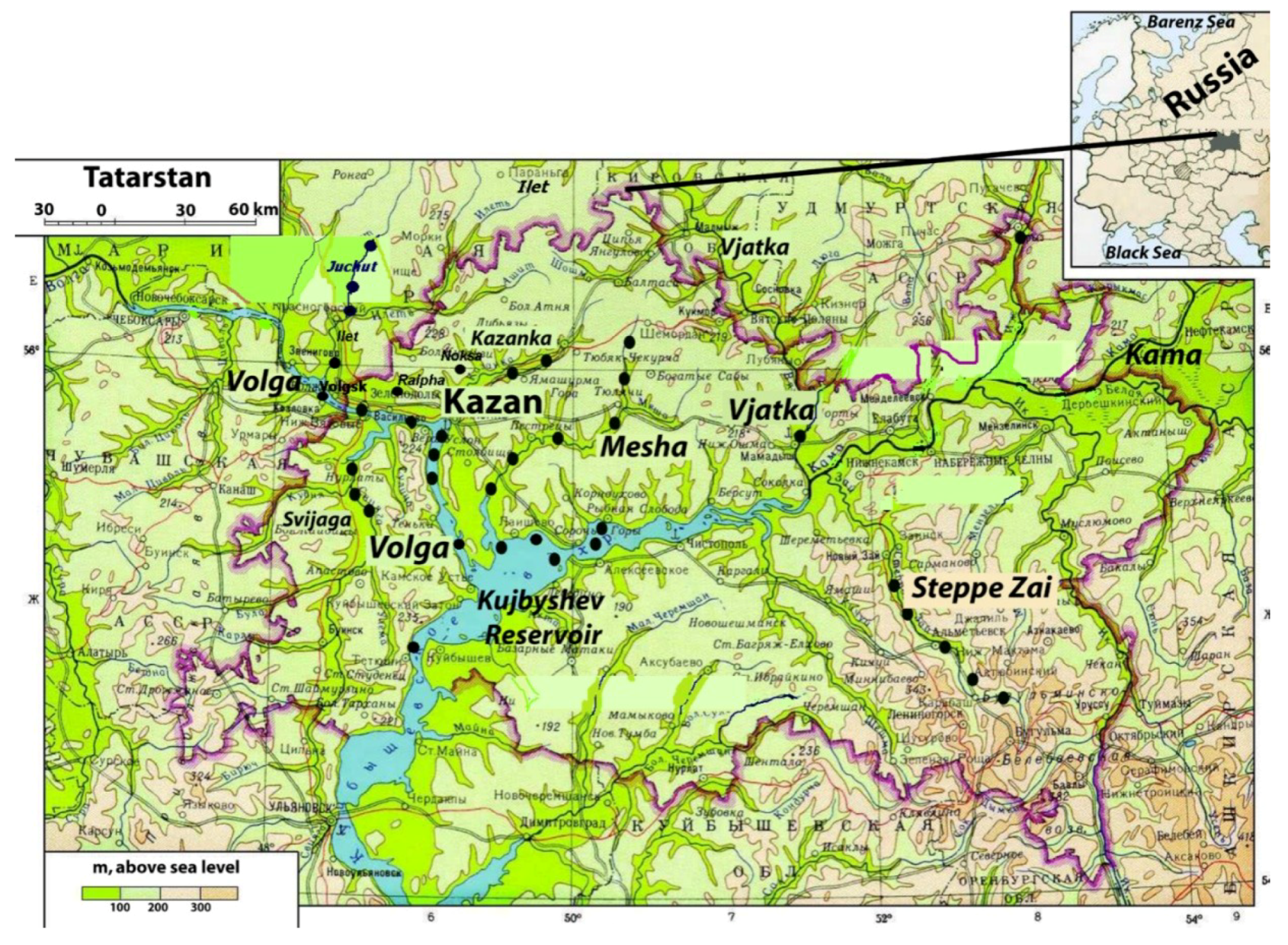
2.1. Study Area

We carried out studies of cilioplankton on different types of water bodies, namely, lakes, rivers, and the reservoir of the Middle Volga basin (Figure 1). The territory of the Middle Volga region is located within the Russian Plain, in the temperate climate zone, at the junction of three zones: broad-leaved forests, southern taiga, and forest–steppe. The study area is cut by large European waterways: the Volga, Kama, and Vjatka rivers, with their numerous tributaries, as well as small and large reservoirs on them [17].
The largest water body considered in the study area is the Kujbyshev Reservoir, which is the result of the closure of the Volga River by the dam of the Kujbyshev Hydroelectric Station in the area of the Zhiguli Mountains. The reservoir was filled from the end of October 1955 to May 1957, when the water level reached a normal impound level. It has a total capacity of 57.3 km3 and a useful capacity of 33.9 km3. The catchment area is 1210 km2, while the surface area reaches 6.15 thousand km2. The maximum width of the reservoir is about 26 km (near the Kama Estuary); its total length is 467 km along the Volga River and 280 km along the Kama River. The average depth is 9.3 m, while the maximum depth reaches 41 m (Volga Hydroelectric Station dam). The total shore length is 2604 km [18].
We conducted the studies in the Kujbyshev Reservoir and its tributaries of different orders: the rivers Vjatka, Steppe Zai, Kazanka, Mesha, Svijaga, Ilet, and its tributary Yushut. We also studied the Raifa Lake for comparison purposes and contrasted the condition of this aquatic ecosystem with other water bodies. Since all investigated water bodies are located within the same region, their hydrochemical characteristics are similar (see Table 1).
There are various anthropogenic sources of pollution of natural waters in this region. The main ones are the following: domestic wastewater; industrial contaminated wastewater; melting snow and rainwater from the territory of towns and factories; drainage water from amelioration systems; surface runoff with melt and rainwater from agricultural lands; and wastewater from livestock complexes and poultry farms [19].
The territories of several cities (Kazan, Naberezhnye Chelny, Nizhnekamsk, Zelenodolsk, and Volzhsk), including engineering, chemical, petrochemical, and processing factories, are located in the catchment area of the Kujbyshev Reservoir. The impact of urban ecosystems manifests itself as the abstraction of water, discharges of industrial and domestic wastewater, and surface runoff of snowmelt and rainwater from their territories. The main pollutants from these facilities are phenols, total petroleum hydrocarbons (TPH), manganese, copper, iron, and nitrogen compounds [19].
Anthropogenic impact on small rivers (Mesha, Svijaga) is mainly due to agricultural facilities, as well as organized discharges of sewage from cities and towns (Steppe Zai, Kazanka, and Vjatka). The Steppe Zai River is additionally affected by oil extraction.
The Ilet River with its tributary Yushut is located in a sparsely populated forest zone, where there are no large towns. Therefore, the anthropogenic impact on these ecological systems is minimal.
Raifa Lake is located on the territory of the Volga–Kama State Nature Reserve and is in pristine condition.
Thus, the objects of study are characterized by different levels of anthropogenic influence ranging from high (Kujbyshev Reservoir) to low (Ilet and Yushut rivers, Raifa Lake).

2.2. Sampling and Analysis Methods

Water samples were collected from May to October during a long period from 1997 to 2004 and from 2018 to 2019, with a frequency of one sample every two weeks or once a month.
Samples of ciliates were collected with a bathometer in amounts of 0.5 L of water at each station. Then, 300 mL of water were taken from the sample and filtered through a membrane filter No. 9 by gravity (without vacuum) to a volume of 10 mL. Next, 0.5 mL from the obtained filtrate were distributed in drops on a glass plate and examined under a microscope to account for small forms (from 15 to 50 μm). The remaining 9.5 mL of water were examined in a Bogorov chamber to count large forms (from 50 to 400 μm). The number of ciliates per 1 m3 was calculated by the formula
N = 66n1 + 3.3n2
where N is the number of ciliates in 1 L (× 1000 = 1 m3), n1 is the number of ciliates in 0.5 mL of the sample for small forms, and n2 is the number of large ciliates in 10 mL of the sample [5].
Species guides [10,20] were used to identify the species. The Shannon–Weaver index [21] was used to assess species diversity. Water quality was assessed by the Pantley–Buck saprobity index [22] modified by Sladecek [23]. The degree of pollution was assessed according to a system commonly adopted in Russia [24,25]. As specified by this system, the water quality is characterized as clean if the saprobity index is less than 1.5, weakly polluted if it is 1.5–2.5, polluted if it is 2.5–3.5, dirty if it is 3.5–4, and extremely dirty if it is greater than 4. A total of 165 water samples were collected and analyzed throughout the study.
In parallel, we performed a hydrochemical analysis to determine the composition of water by 19 components: pH, hardness, mineralization, bicarbonates, oxygen dissolved in water, biological and chemical oxygen demand BOD5, COD, N–NO2, N–NO3, N–NH4+, chlorides, sulfates, total iron, phenols, total petroleum hydrocarbons, Cu2+, Zn2+, total Cr, and Mn2+. Moreover, we performed an analysis of long-term (over the past 15 years) hydrochemical information. To assess the water quality by chemical indicators, we calculated the specific combinatoric index of water pollution (SCIWP), which takes into account the multiplicity and frequency ratio of exceeding the maximum permissible concentrations (MPC) [25].

2.3. Data Analysis Methods

To analyze the data as a biological indicator, we calculated the species diversity index (H) based on the number of ciliates; its values varied from 0 to 4.5. All studied water bodies according to H were characterized as “moderately polluted” and “dirty”, that is, they were divided into two classes of water quality, the first one being clean (0) and the second one, dirty (1). The database included 126 observations: 85 clean (0) and 41 dirty (1). Class 0 is characterized by a higher species diversity of cilioplankton compared to class 1.
We applied logistic regression to assess the relationship between the class of water quality (clean—0 or dirty—1) determined by the species diversity index (H), calculated for the cilioplankton, and data obtained from the hydrochemical analysis.
The binary logistic regression is a type of regression used when the dependent variable is a dichotomous one and the independent variables are quantitative data.
The binary logistic regression model with several independent variables is given as
p = P ( Y = 1 | X ) = 1 1 + exp ( z )
z = β 0 + β 1 × X 1 + β 2 × X 2 + β m × X
where p is the probability that Y = 1 for a given set of values of X, and z is the standard regression equation [26].
Logical regression is a popular statistical method used in biology and ecology [27,28,29]. It is a standard analysis method in situations where the dependent variable (Y) is dichotomous, taking the values 0 and 1.
In the case considered in the study, the dependent variable (Y) is the class of water quality (clean—0 or dirty—1). The independent variables (predictors) are 19 chemical indicators of water quality. During the initial data analysis, we found that some variables have a pronounced asymmetric distribution; in this connection, we preliminarily calculated the logarithm of these data. The entire original sample was randomly divided into two sets of 80% (training data) and 20% (test data).
A stepwise procedure of inclusions with exclusions of “weak” predictors was applied to determine the significant variables that most strongly affect the resulting variable.
The quality of the logistic regression model was assessed by ROC analysis (Receiver Operating Characteristic). The predictive capability of the constructed model was assessed by 10-fold cross-validation with five repeats.
The model construction and all the calculations were conducted using programs written in R. We used the standard R libraries and several packages, such as vegan, ROCR, boot, ggplot2, and caret [30].

3. Results

3.1. Hydrochemical Features of the Objects of Study

The chemical composition of the water in the investigated water bodies is given in Table A1, Table A2 from Appendix A.
The water of the rivers Ilet, Kazanka, Steppe Zai, and Noksa features elevated hardness and mineralization. The mineralization of the water in the Kazanka and Ilet rivers (351 to 1457 mg/L) is mainly due to sulfates and is associated with the intensive discharge of groundwater. The mineralization of water in the Steppe Zai River (429 to 1480 mg/L) is determined by the high content of chlorides coming from groundwater contaminated as a result of oil extraction activities on the catchment of this river. The water of the Vjatka River is characterized by lower mineralization (113 to 511 mg/L); the same is true for the Kujbyshev Reservoir and Raifa Lake (171 to 263 mg/L). Other indicators are mainly connected to factors of anthropogenic nature.
The Kujbyshev Reservoir at most sites was classified as “dirty” according to its hydrochemical composition. The main contribution to the surface water pollution is made by copper compounds, organic compounds (in terms of BOD5 and COD), ammonium nitrogen, nitrite nitrogen, and TPH. The frequency of exceeding the MPC of these substances ranges from 30 to 50%. The oxygen regime in the reservoir was satisfactory throughout the study.
The water of Kazanka and Steppe Zai rivers was also classified as dirty. The main chemical indicators of pollution include organic matter (in terms of COD and BOD5), nitrite nitrogen, copper and iron, TPH, ammonium nitrogen, and sulfates. Chlorides are significant indicators only in the Steppe Zai River.
The rivers Vjatka, Mesha, Svijaga, and Noksa were classified as highly polluted by their water quality. Organic substances (in terms of COD), sulfates, and copper are characteristic indicators in these rivers. Additionally, nitrite nitrogen appeared as a characteristic indicator in the Noksa River. We observed a deterioration of the oxygen regime only in the Noksa River in summer.
The degree of pollution of the Raifa Lake is also very high; we detected an increased content of organic substances (in terms of COD and BOD5), as well as compounds of both iron and copper.
The Ilet and Yushut rivers were classified as polluted. In these rivers, we found an increased content of sulfates, iron, and copper. In the Yushut, we detected organic substances leading to characteristic pollution (in terms of COD).
Moreover, a section of the Kujbyshev Reservoir was characterized as extremely dirty. This corresponds to the wastewater discharge area at the Mari El Pulp and Paper Mill (MPPM), near the town of Volzhsk. Water pollution by phenols, organic substances (in terms of COD and BOD5), and ammonium nitrogen compounds were persistently detected at this site. The complete absence of oxygen in the water should also be notated.
Thus, the objects of research were classified in accordance with their water quality and ranked from polluted to extremely dirty.

3.2. Features of the Development of Ciliates

The surveyed water bodies and watercourses can be distinguished by a wide variety in their infusoria fauna and the ranges of fluctuation in their numbers (see Table 2). The number of species of ciliates and their abundance are the most important indicators characterizing the condition of ecosystems, since a sudden external influence leads ciliates to reduce their number, whereas a prolonged one cause changes in species composition, along with a simplification of trophic structure.
In the examined water bodies, we identified 156 species of ciliates (see Table 2). The Kujbyshev Reservoir shows the greatest species diversity, with 99 species. The least diversity was detected in the area of wastewater discharge at the MPPM: only 10 species.
Among the examined rivers, the largest number of species was found in the Kazanka River (111 species), and the smallest in the Noksa river (13 species).
A low species diversity and little variation in the number of species and abundance are typical for water bodies that are less affected by anthropogenic factors (background condition) and have a good oxygen regime (7.5–10.7 mg/L), and low content of organic (BOD5 = 0.42–1.85 mgO2/L) and biogenic (PO43− = 0–0.016 mg/L) substances. The most frequently occurring intervals (MFOI) for the number of species in such ecosystems did not exceed 7–10, and the corresponding numbers were 200.0–1000.0 thousand N/m3. The Shannon species diversity index (H) was high enough (2.0 to 3.3). The structure-forming complex of cilioplankton was represented by Cyclidium sp, Halteria grandinella (Müller, 1773), Urotricha pelagica (Kahl, 1935), and Limnostrombidium pelagicum (Kahl, 1932). The saprobity index (S) varied within from 1.3 to 2.1, which corresponds to waters going from conditionally clean to moderately polluted.
A significant variation in the number of cilioplankton was detected in rivers that were characterized as “dirty” due to increased contents of organic substances in terms of both BOD5 (1.0–4.9 mgO2/L) and COD (9.2–26.8 mgO2/L), ammonium nitrogen (0.0–0.49 mg/L), nitrite nitrogen (0.024–0.096 mg/L), as well as metals, such as Cu (0.0–4.7 μg / L) and Cr (1.1–3.4 μg/L), while showing a satisfactory oxygen regime (6.8–12.8 mg/L). This is an indication of restructuration in the biocoenoses of these rivers throughout a season. The MFOI of cilioplankton abundance in such rivers ranged from 1000.0 to 3000.0 thousand N/m3, and the number of species was 1–10. The dominant complex was represented by the following species: Coleps hirtus (Nitzsch, 1817), H. grandinella, Askenasia volvox (Eichwald, 1852) Blochmann, 1895, Vorticella spp. The H index varied from 0.65 to 2.8. At the same time, the S index varied from 1.97 to 2.67, which corresponds to an intermediate condition between moderately polluted and dirty water.
In eutrophic water bodies with high contents of organic substances in terms of both BOD5 (2.0–4.2 mgO2/L) and COD (17.0–28.0 mgO2/L), ammonium nitrogen (0.19–0.82 mg/L), and nitrite nitrogen (0.016–0.167 mg/L), the number of cilioplankton reached 132.0 million N/m3, while the MFOI were 2000.0–20,000.0 thousand N/m3, and the number of species was 4–6. The cilioplankton community was based on the following species: Rimostrombidium lacustris (Foissner, Skogstad, and Pratt, 1988), T. fluviatile, H. grandinella, Monodinium balbiani (Fabre-Domergue, 1888), U. pelagica, C. hirtus. The H index ranged from 1.6 to 2.0. The water quality determined by S corresponded to slightly polluted waters, namely 2.0 to 2.2.
The development of ciliates was found to be suppressed under severe toxic conditions (TPH = 0.16–0.76 mg/L, phenols = 0.024–0.18 mg/L), organic pollution (BOD5 = 11.4–34.1 mgO2/L, COD = 37.8–86.2 mgO2/L), high content of ammonium nitrogen= 0.6–2.2 mg/L, and low oxygen content (0.0–4.9 mg/L) in water. In such water bodies, there were one to three species of ciliates, and their numbers did not exceed 6.0 thousand N/m3, but reached 4000.0 thousand N/m3 during short periods. The MFOI of abundance in such ecosystems are 0–1000, while the number of species ranges from 0 to 3. Here, the plankton may contain species not requiring oxygen, such as Stentor polymorphus (Müller 1773) Ehrenberg, 1830, Paramecium putrinum (Claparede and Lachmann 1858), and Carchesium polypinum (Linnaeus, 1758). The H index varied from 0.72 to 2.26; and S ranged from 2.7 to 3.1, which corresponds to polluted–dirty waters.
At the same time, no ciliates at all were found at extremely high levels of pollution, namely complete absence of oxygen, very high content of organic substances (BOD5 = 34.1 mgO2/L, COD = 86.2 mgO2/L), ammonium nitrogen= 2.2 mg/L, TPH = 0.76 mg/L, phenols = 0.18 mg/L, and some metals (Al = 139 μg/L, Mn = 207 μg/L).
According to the species diversity index (H), calculated for the number of cilioplankton (see Table 2), all the examined water bodies were classified as moderately polluted and dirty (H > 3 corresponds to clean, H from 1 to 3 is moderately polluted, and H < 1 is dirty).

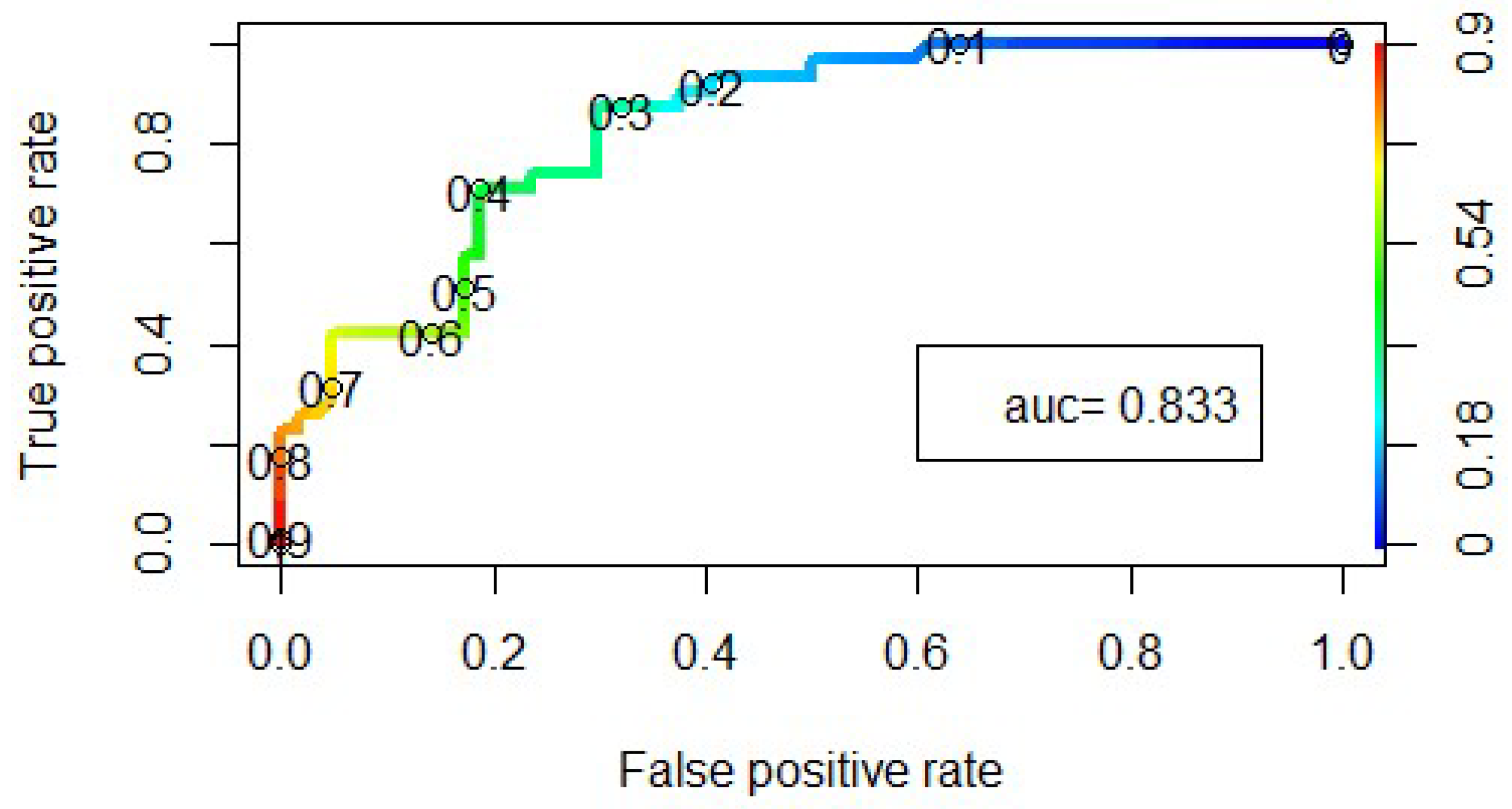
3.3. Statistical Analysis Logistic Regression Model

We used logistic regression to study the relationship between hydrochemical indicators that characterize a water body and its water quality, which is classified as “clean—0/dirty—1” according to the species diversity index.
Using a stepwise procedure, we chose eight of the most important predictors: temperature, chlorides, mineralization, bicarbonates, biological oxygen consumption, nitrates, iron, and total petroleum hydrocarbons.
Based on the eight selected variables, we simulated the probability of an object falling into class 1. As a result, we obtained the following logistic regression equation:
{ p = P ( Y = 1 | X ) = 1 1 + exp ( z ) z = 1.29 0.7 × X 1 + 1.13 × X 2 + 1.85 × X 3 1.21 × X 4 + 0.98 × X 5 + 1.38 × X 6 0.84 × X 7 1.9 × X 8
where X1 is temperature, X2 stands for chlorides (Cl), X3 for mineralization (Min), X4 for hydrocarbonates (HCO3), X5 for biological oxygen demand (BOD5), X6 for nitrates (NO3), X7 for iron (Fe), and X8 for total petroleum hydrocarbons.
Table 3 contains the estimated coefficients, standard errors, and Wald test statistics (Z value) for the logistic regression. All coefficients in the model are statistically significant. The obtained coefficients reflect the contribution of the corresponding predictor.
The optimal cutoff threshold for the probability was set to 0.35. This cutoff threshold was found as the intersection of three important indicators of the model: specificity, sensitivity, and efficiency. An analysis of the training sample showed that the specificity and sensitivity for the constructed model was 78%, while the accuracy was 77%. An analysis of the test sample showed that the accuracy of the model is 74%, the specificity is 52%, and the sensitivity is 85%.
To assess the quality of the resulting logistic regression model, we constructed the ROC curve in coordinates x = 1 − Specificity and y = Sensitivity, which reflects the quality of the logistic model (Figure 2). The Area Under the Curve AUC = 0.833 characterizes the quality of the model as good.
Using 10-fold cross-validation with five repeats, it was shown that the model has a prediction accuracy of 75%. This positively characterizes the resulting model.

4. Discussion

According to their chemical parameters, the studied water bodies were characterized as polluted and dirty, due mainly to pollutants of anthropogenic origin. The most significant among them were organic substances (in terms of both COD and BOD5), sulfates, chlorides, nitrogen compounds (ammonium nitrogen, nitrates, nitrites), as well as heavy metals (iron, copper, manganese, aluminum), total petroleum hydrocarbons, and phenols.
The concentrations of organic substances varied over the observation period from 1.4 to 208.3 mgO2/L in terms of COD and from 0.3 to 48.27 mgO2/L in terms of BOD5. The lowest values were observed in small rivers (Svijaga, Yushut, Ilet)—the highest, in the Kuibyshev Reservoir in the discharge area of the MPPM.
The sulfate content in water was 3.3–835.7 mg/L. The minimum values were registered in the Steppe Zai, the maximum ones in the Kazanka. The chloride content in natural water was 0.0–413.0 mg/L, with the minimum values corresponding to the Yushut and the maximum to the Steppe Zai. The concentration of ammonia nitrogen varied from 0.0 to 4.8 mg/L; the maximum values were registered in the Steppe Zai. The nitrate–nitrogen content was 0.0–9.46 mg/L, and nitrite nitrogen was 0.0–0.19 mg/L. The maximum concentrations of nitrates nitrogen were recorded in the discharge area of the MPPM and the Noksa River; for nitrites’ nitrogen, the maximum values were found in the Kujbyshev Reservoir. The content of heavy metals in water varied in the following ranges: iron—0.0–1.1 mg/L, copper—0.0–30.5 μg/L, and manganese—0.0–303.0 mg/L. The highest concentrations of metals were detected in the Steppe Zai (for iron), the Kujbyshev Reservoir (for copper), and the discharge area of the MPPM (for manganese).
The content of total petroleum hydrocarbons and phenols varied in the interval 0.0–0.76 mg/L and 0.0–0.18 mg/L, respectively. The highest concentrations of these substances were recorded in the discharge area of the MPPM. Another important indicator of water quality is the content of dissolved oxygen. In the investigated water bodies, this indicator ranged from 0.0 to 14.57 mg/L. The lowest values were found in the area of the MPPM.
The SCIWP calculated by chemical parameters varied in the studied water bodies from 2.66 to 11.35. The lowest values were recorded in the Ilet and Yushut rivers; this characterizes these rivers as contaminated or polluted. The highest value of the index was in the area of the MPPM, which allowed attributing this section of the Kujbyshev Reservoir to extremely dirty.
The other sections of the Kujbyshev Reservoir, as well as the Steppe Zai and Kazanka correspond to the dirty interval (SCIWP 4.1–4.63). The Noksa, Svijaga, Mesha, Vjatka, and Raifa Lake were rated as highly polluted (SCIWP 3.34–3.64). This means that, in terms of water quality, most of the examined water bodies in the Middle Volga fall into the category of highly polluted and dirty.
The water-quality assessment by the saprobity index showed that most water bodies correspond to the category of slightly polluted. Moreover, one object was classified as conditionally clean–slightly polluted (Raifa Lake); the Noksa River was rated as slightly polluted, the Steppe Zai River as contaminated, and the wastewater discharge area at the MPPM as contaminated to dirty. According to the index of species diversity, most water bodies fall into the category of moderately polluted (=slightly polluted) waters, the Vjatka river was clean, and the wastewater discharge area at the MPPM was rated as dirty. Therefore, the assessment of water quality by the saprobity index does not coincide with the assessment by chemical indicators and, for most water bodies, the former was found to be better than the former. Another disadvantage of the saprobity index is that it cannot be used to evaluate extremely dirty ecosystems, where ciliates are completely absent. In this case, the species diversity index (H) is more appropriate, as it takes into account the qualitative and quantitative development of organisms in the environment.
The constructed model of logistic regression can determine the quality of water bodies and classify them as “clean/dirty”. For this purpose, it uses the species diversity index (H) of cilioplankton and seven significant chemical predictors of both natural origin (mineralization, hydrocarbonates, and chlorides) and natural-anthropogenic origin (organic matter content in terms of BOD5, nitrates, total petroleum hydrocarbons, iron), as well as a physical factor, the water temperature, which mostly determines the development of cilioplankton.
Previous studies have proven the existence of dependence between the indicators of cilioplankton and the content of organic substances both in surface water [15,16,31,32] and in wastewater [33]. However, it has been noted that high concentrations of organic substances (in terms of COD and BOD) and ammonium salts adversely affect the development of ciliates [34]. The most toxic for ciliates are high concentrations of ammonium and salts of heavy metals: cadmium, copper, chromium, lead, and nickel [35,36]. Moreover, it has been noticed that changes in the ecological and morphological parameters of ciliates occur under the influence of nitrates, in particular, a decrease in body size, contractile vacuole, and peristome [37].
The highest contents of ammonium and nitrates (4.8 and 9.6 mg/L), as well as organic substances (208.3 mgO2/L as per COD and 48.3 mgO2/L as per BOD5) were detected in the discharge area at the MPPM. Ciliates were absent at such critical values. In the Mesha River, where the concentration of ammonium (N-NH4+) was 9.4 mg/L, the number of ciliates was only 283.0 thousand N/m3. In the Svijaga River, where the nitrate (N-NO3) content is 3.5–7.4 mg/L and ammonium (N-NH4+) is 0.1–0.5 mg/L, we detected 1–2 species of ciliates with 400.0–1000.0 thousand N/m3. At the same time, small-sized forms of infusoria, such as R. lacustris and H. grandinella, were present in the samples. Thus, when the concentration of nitrogen in the water increases, the species diversity of infusoria and their abundance decrease, and small-sized forms prevail. These patterns were noted earlier by other researchers [38,39,40].
The Shannon species diversity index calculated for the number of cilioplankton has been suggested by other researchers [31,32] for the assessment of the quality of water bodies of different types (in particular, seawater). It has been pointed out that protozoan community diversity indices could be used as indicators that are more effective in biomonitoring aquatic ecosystems. This is because infusoria have a short life cycle and, as a result, the community response to external influence is rapid.
Recently, new approaches based on synecological methods have been introduced in addition to traditional methods for assessing water quality using infusoria (saprobity index, index of species diversity). We can mention, in particular, a method of functional diversity of infusoria, which is based on the structural features of ciliates and the type of nutrition [13]. The use of this technique in different communities of infusoria (benthic, epiphytic, planktonic) showed that the functional diversity of communities has a high potential for monitoring the ecological condition of the aquatic environment [41,42]. In our opinion, these methods, based on the approaches of functional and evolutionary ecology, are designed to study the condition of an ecosystem as a whole and we plan to consider these methods in future studies.

5. Conclusions

Water bodies of the Middle Volga region are subjected to varying degrees of anthropogenic impact. This affects the quality of surface water, which can be rated from contaminated to extremely dirty.
Various cilioplankton communities develop in water bodies with different levels of pollution. They differ in species composition and abundance. According to the saprobity index (S) and the species diversity index (H), the water quality was rated as moderately polluted in most water bodies.
The statistical analysis showed the existence of a relationship between the water quality of a water body (classified as "clean/dirty" according to the species diversity index (H) of cilioplankton) and hydrochemical indicators that characterize the water quality. Using logistic regression, we determined eight significant predictors: water temperature, chlorides, mineralization, hydrocarbonates, BOD5, nitrates, iron, and total petroleum hydrocarbons. These are the most significant when determining the water quality class by the Shannon index calculated for the number of ciliates.
Qualitative and quantitative indicators of development of ciliates, as well as indices calculated on their basis, allow assessing with a very high level of accuracy the water quality and the condition of aquatic ecosystems in general. In particular, the Shannon index calculated for the number of ciliates can be successfully used for ranking water bodies as “clean/dirty”.
Thus, ciliates as an object of bioindication are a very convenient and promising group for biomonitoring needs, including the implementation of methods of the Water Framework Directive.

Author Contributions

Conceptualization: T.K. and N.S.; methodology, T.K. and N.S.; formal analysis, T.K. and T.N.; investigation, T.K. and T.N.; resources, T.K. and N.S.; writing—original draft preparation, T.K., T.N., and N.S.; writing—review and editing, T.K. and N.S.; funding acquisition, N.S.

Funding

This research was funded by the Russian Foundation for Basic Research and the Government of the Republic of Tatarstan (project No. 18-44-160027).

Conflicts of Interest

The authors declare no conflict of interest.

Appendix A

Table A1. Hydrochemical composition (mg/L, * μg/L) of the Ilet, Yushut, Kazanka, Svijaga, Mesha, and Steppe Zai rivers.
Water BodyIletYushutKazankaSvijagaMeshaSteppe
Zai
pH7.53–8.03
7.7 ± 0.1
7.36–8.0
7.63 ± 0.08
7.0–8.6
7.8 ± 0.3
7.5–8.2
8.1 ± 0.7
7.35–8.35
8.0 ± 0.4
7.3–8.5
7.9 ± 0.06
O27.26–12.4
9.15 ± 2.1
6.18–10.67
8.64 ± 0.49
7.5–14.57
9.5 ± 3.6
10.2–13.1
10.9 ± 1.7
6.79–8.14
8.0 ± 1.1
2.63–12.53
8.9 ± 0.1
Cl7.09–11.7
10.5 ± 1.1
0.0–9.0
6.8 ± 1.2
15.1–53.2
9.2 ± 3.2
10.0–19.9
24.4 ± 5.7
0.0–10.5
11.11 ± 1.36
15.2–413.0
156.7 ± 7.2
SO42−134.5–694.0
455.8 ± 100.37
19.0–619.4
101.3 ± 64.9
59.3–835.7
536.1 ± 247.2
65.0–200.0
125.50 ± 12.56
62.4–192.1
120.8 ± 66.2
3.3–345.8
129.9 ± 4.2
Mineralization444.1–1135.3
955.1 ± 129.9
162.4–251.4
271.8 ± 61.7
351.3–1456.7
1082.8 ± 96.4
478.0–630.0
659.5 ± 65.9
245.0–810.5
460.9 ± 80.8
429.2–1479.9
770.8 ± 42.4
Hardness11.1–18.0
14.5 ± 1.1
2.8–12.8
6.56 ± 1.66
3.9–93.0
14.6 ± 4.5
3.0–4.0
8.4 ± 1.1
3.0–9.3
5.7 ± 1.1
4.6–14.3
9.2 ± 0.5
HCO3192.2–281.9
336.3 ± 15.9
115.9–149.5
139.65 ± 4.98
34.9–350.5
240.4 ± 63.1
278.2–366.1
247.8 ± 114.7
134.2–363.1
218.9 ± 17.6
68.7–497.3
326.9 ± 8.9
COD10.6–12.1
12.1 ± 0.6
11.0–33.3
22.43 ± 2.38
11.0–39.8
23.4 ± 0.6
1.4–28.6
16.6 ± 2.4
8.1–19.1
13.3 ± 1.1
8.7–42.0
24.1 ± 0.5
BOD50.42–1.53
1.1 ± 0.2
0.65–2.09
1.26 ± 0.16
1.7–7.9
3.74 ± 0.12
1.7–3.2
2.5 ± 0.1
1.0–1.79
1.1 ± 0.1
0.29–7.04
2.22 ± 0.9
N-NH4+0.05–0.17
0.10 ± 0.01
0.16–0.33
0.19 ± 0.02
0.0–3.8
0.351 ± 0.05
0.1–0.6
0.4 ± 0.06
0.0–0.48
0.06 ± 0.14
0.0–4.8
0.78 ± 0.06
N-NO20.0–0.01
0.01 ± 0.0
0.01–0.02
0.01 ± 0.0
0.0–0.05
0.02 ± 0.0
0.0–0.2
0.1 ± 0.02
0.01–0.19
0.081 ± 0.088
0.0–0.7
0.12 ± 0.01
N-NO30.17–2.69
1.160.55
0.01–3.28
0.53 ± 0.28
0.0–1.43
0.37 ± 0.04
0.4–7.4
4.0 ± 0.8
0.07–1.93
1.04 ± 0.13
0.06–10.04
2.67 ± 0.13
PO43−0.0–0.12
0.04 ± 0.02
0.013–0.12
0.04 ± 0.01
0.0–0.1
0.02 ± 0.0
0.1–0.6
0.3 ± 0.06
0.0–0.19
0.05±0.02
0.0–1.65
0.24 ± 0.02
Fe0.06–0.28
0.13 ± 0.04
0.07–0.51
0.24 ± 0.06
0.0–0.36
0.05 ± 0.01
0.0–0.2
0.10 ± 0.03
0.0–0.27
0.02 ± 0.02
0.01–1.1
0.05 ± 0.0
Cu*4.6–8.3
6.12 ± 0.75
0.1–2.7
1.0 ± 0.37
0.0–22.5
4.07 ± 0.37
2.0–7.0
3.4 ± 0.58
0.0–6.3
2.2 ± 1.21
0.0–9.7
2.24 ± 0.09
Mn*6.2–14.0
8.56 ± 1.41
7.7–126.0
41.9 ± 11.7
2.4–3.5
2.7 ± 0.27
12.1–171.7
84.8 ± 16.7
1.4–94.0
14.3 ± 7.4
3.7–142.8
28.2 ± 3.9
TPH0.0–0.09
0.04 ± 0.02
0.004–0.021
0.016 ± 0.00
0.0–0.27
0.09 ± 0.01
0.0–0.6
0.2 ± 0.07
0.0–0.04
0.01 ± 0.0
0.0–0.09
0.03 ± 0.0
Phenols0.0–0.0
0.0 ± 0.0
0.0–0.001
0.0 ± 0.0
0.0–0.004
0.001 ± 0.00
0.0–0.0
0.0 ± 0.0
0.0–0.0
0.0 ± 0.0
0.0–0.005
0.0 ± 0.0
SCIWP2.662.734.43.643.64.1
Water qualityPollutedPollutedDirtyHighly
polluted
Highly
polluted
Dirty
The numerator is min–max, the denominator is average ± ∆; TPH—total petroleum hydrocarbons; SCIWP—the specific combinatoric index of water pollution.
Table A2. Hydrochemical composition (mg/L *µg/L) of the Kujbyshev Reservoir, the rivers Vjatka and Noksa, and Raifa Lake.
Water BodyVjatkaNoksa Raifa LakeKujbyshev ReservoirMPPM
pH7.71–8.47
8.05 ± 0.09
7.27–8.25
7.80 ± 0.14
7.3–9.2
8.29 ± 0.17
6.5–8.65
7.7 ± 0.1
7.05–7.64
7.29 ± 0.07
O26.57–13.59
9.68 ± 0.3
4.44–11.38
7.89 ± 1.19
6.3–13.8
8.67 ± 0.64
5.59–13.6
9.7 ± 0.6
0.0–3.05
0.95 ± 0.43
Cl1.1–56.7
8.32 ± 1.32
33.2–51.1
43.87 ± 3.06
10.0–17.3
11.9 ± 0.82
9.2–78.7
22.3 ± 2.2
10.2–37.4
25.52 ± 3.37
SO42−5.0–133.5
43.97 ± 4.77
107.6–552.4
265.8 ± 80.6
7.1–29.0
13.18 ± 1.97
12.6–414.3
79.2 ± 14.1
47.6–480.3
175.64 ± 59.24
Mineralization112.9–511.0
277.26 ± 17.98
546.9–1211.9
787.7 ± 94.5
170.6–263.4
218.6 ± 11.86
119.3–607.2
308.7 ± 17.9
333.8–1021.4
526.11 ± 93.64
Hardness1.2–5.2
2.94 ± 0.20
7.6–13.04
9.44 ± 0.77
1.36–3.4
2.45 ± 0.18
1.6–7.8
3.5 ± 0.2
3.0–6.2
4.43 ± 0.39
HCO359.5–244.6
156.07 ± 10.56
311.2–755.1
443.75 ± 67.02
86.1–249.0
143.5 ± 13.46
10.6–308.2
133.7 ± 9.7
146.4–281.9
215.84 ± 18.65
COD16.0–43.8
25.07 ± 1.20
10.0–24.1
20.02 ± 2.62
16.9–35.9
24.9 ± 1.8
7.3–47.7
29.4 ± 2.3
37.7–208.3
94.3 ± 21.5
COD50.66–4.73
2.1019
1.58–1.93
1.74 ± 0.08
0.5–7.1
2.73 ± 0.49
0.3–4.29
3.1 ± 0.7
11.36–48.27
28.01 ± 6.06
N-NH4+0.0–0.91
0.32 ± 0.04
0.05–0.42
0.19 ± 0.06
0.018–0.43
0.019 ± 0.04
0.0–1.17
0.35 ± 0.07
0.54–2.19
1.25 ± 0.21
N-NO20.0–0.03
0.01 ± 0.00
0.029–0.096
0.06 ± 0.01
0.0–0.041
0.038 ± 0.03
0.0–0.19
0.03 ± 0.01
0.0–0.02
0.008 ± 0.00
N-NO30.01–1.41
0.30 ± 0.06
0.99–9.46
3.56 ± 1.57
0.0–0.9
0.19 ± 0.09
0.0–1.3
0.45 ± 0.26
0.0–9.46
1.79 ± 1.42
PO43−0.0–0.05
0.02 ± 0.00
0.0–0.28
0.11 ± 0.04
0.0–0.18
0.05 ± 0.01
0.0–0.29
0.05 ± 0.01
0.0–0.081
0.016 ± 0.01
Fe0.01–0.85
0.21 ± 0.04
0.11–0.20
0.14 ± 0.03
0.02–0.35
0.19 ± 0.03
0.0–0.62
0.13 ± 0.02
0.136–0.237
0.189 ± 0.01
Cu*0.0–6.6
2.62 ± 0.25
0.0–4.7
3.13 ± 1.57
0.0–14.0
3.15 ± 1.0
0.0–30.5
2.98 ± 0.46
2.9–7.5
4.25 ± 0.57
Mn*5.6–52.2
25.37 ± 4.62
14.0–20.0
18.0 ± 2.0
0.0–59.0
12.1 ± 5.3
0.0–280.0
49.2 ± 9.4
7.0–303.0
160.74 ± 38.70
TPH0.0–0.09
0.03 ± 0.00
0.0–0.19
0.06 ± 0.01
0.0–0.02
0.008 ± 0.0
0.0–0.5
0.099 ± 0.030
0.059–0.76
0.27 ± 0.11
Phenols0.0–0.004
0.001 ± 0.00
0.0–0.001
0.0 ± 0.0
0.001–0.005
0.001 ± 0.00
0.0–0.004
0.001 ± 0.00
0.0034–0.18
0.073 ± 0.03
SCIWP3.63.343.454.6311.35
Water qualityHighly
polluted
Highly
polluted
Highly
polluted
DirtyExtremely
dirty
The numerator is min–max, the denominator is average ± ∆.

References

  1. Directive 2000/60/EC of the European Parliament and of the Council of 23 October 2000 Establishing a Framework for Community Action in the Field of Water Policy. Directive 2000/60/EC of the European Parliament ... Action in the Field of Water Policy. Available online: https://www.eea.europa.eu/policy-documents/directive-2000-60-ec-of (accessed on 29 October 2019).
  2. Morduhaj-Boltovskaya, E.D.; Sorokin, Y.I. Pitanie infuzorij vodoroslyami i bakteriyami (Feeding of ciliates on algae and bacteria). Tr. Inst. Biol. Vnutr. Vod. 1965, 8, 12–14. (In Russian) [Google Scholar]
  3. Mamaeva, N.V. Ciliates of the Volga River Basin; Nauka: Moscow, Russia, 1979; p. 150. (In Russian) [Google Scholar]
  4. Mamaeva, N.V.; Kopylov, A.I. To study the nutrition of freshwater infusoria. Cell Tissue Biol. 1978, 20, 472–476. (In Russian) [Google Scholar]
  5. Obolkina, L.A. Planktonic Ciliates of Lake Baikal. Hydrobiologia 2006, 568, 193–199. (In Russian) [Google Scholar] [CrossRef]
  6. Porter, K.G.; Sherr, E.B.; Sherr, B.F.; Pace, M.; Sanders, R.W. Protozoa in Planktonic Food Webs1, 2. J. Protozool. 1985, 32, 409–415. [Google Scholar] [CrossRef]
  7. Berninger, U.G.; Finlay, B.J.; Canter, H.M. The Spatial Distribution and Ecology of Zoochlorellae-Bearing Ciliates in a Productive Pond 1. J. Protozool. 1986, 33, 557–563. [Google Scholar] [CrossRef]
  8. Berninger, U.G.; Finlay, B.J.; Kuuppo-Leinikki, P. Protozoan control of bacterial abundances in freshwater. Limnol. Oceanogr. 1991, 36, 139–147. [Google Scholar] [CrossRef]
  9. Beaver, J.R.; Crisman, T.L. The role of ciliated protozoa in pelagic freshwater ecosystems. Microb. Ecol. 1989, 17, 111–136. [Google Scholar] [CrossRef]
  10. Foissner, W.; Berger, H.; Schaumdurg, J. Identification and Ecology of Limnetic Plancton Ciliates; Bayerisches Landesamtes für Wasserwirtschaft Munchen: Munchen, Germany, 1999; p. 793. [Google Scholar]
  11. Gates, M.A. Quantitative importance of ciliates in the planktonic biomass of lake ecosystems. Hydrobiologia 1984, 108, 233–238. [Google Scholar] [CrossRef]
  12. Bykova, S.V. Free-living Ciliates in the deep-water part of the Kama river reservoirs. Trans. IBIW 2019, 85, 23–43. (In Russian) [Google Scholar] [CrossRef]
  13. Weisse, T. Functional diversity of aquatic ciliates. Eur. J. Protistol. 2017, 61, 31–358. [Google Scholar] [CrossRef]
  14. Weisse, T. Freshwater ciliates as ecophysiological model organisms—lessons from Daphnia, major achievements, and future perspectives Freshwater ciliates as ecophysiological model organisms – lessons from Daphnia, major achievements, and future perspectives. Arch. Hydrobiol. 2006, 167, 371–402. [Google Scholar] [CrossRef]
  15. Xu, H.; Zhang, W.; Jiang, Y.; Yang, E.J. Use of biofilm-dwelling ciliate communities to determine the environmental quality status of coastal waters. Sci. Total Environ. 2014, 470, 511–518. [Google Scholar] [CrossRef] [PubMed]
  16. Liu, H.; Huang, L.; Tan, Y.; Song, X.; Huang, J. Composition and distribution of ciliates inner and outer of Daya Bay, China. Acta Ecol. Sin. 2010, 30, 288–291. [Google Scholar] [CrossRef]
  17. Ministry of Ecology of the Republic of Tatarstan. Report on the State of Natural Resources and Environmental Protection of the Republic of Tatarstan in 2002; Ministry of Ecology of the Republic of Tatarstan: Kazan, Russia, 2003; p. 355. (In Russian)
  18. Institute of Ecology of the Volga Basin. Kuibyshev Reservoir (Scientific Information Guide); Institute of Ecology of the Volga Basin: Tolyatti, Russia, 2008; p. 123. (In Russian) [Google Scholar]
  19. Nikanorov, A.M.; Zakharov, S.D.; Bryzgalo, V.A.; Zhdanova, G.N. The Rivers of Russia. Part III. Rivers of the Republic of Tatarstan (Hydrochemistry and Hydroecology); Hydrochemical Institute: Rostov-on-Don, Russia, 2010; p. 192. (In Russian) [Google Scholar]
  20. Kahl, A. Urtiere oder Protozoa. I. Wimpertiere oder Ciliata (Infusoria). Die Tierwelt Angrenzenden Meerest. 1935, 30, 651–886. [Google Scholar]
  21. Shannon, C.E.; Weaver, W. The Mathematical Theory of Communication; University of Illinois Press: Champaign, IL, USA, 1949; p. 117. [Google Scholar]
  22. Pantle, R.; Buck, H. Die biologische Uberwachung der Gewasser und die Darstellung der Ergebnisse. Gas Wasserfach 1955, 96, 604. [Google Scholar]
  23. Sladeček, V. System of Water Quality from Biological Point of View; Schweizerbart’sche Verlagsbuchhandlung: Stuttgart, Germany, 1973; p. 218. [Google Scholar]
  24. FGBU “GKHI”. Organization and Conduct of Monitoring Observations of the State and Pollution of Surface Water, Guidance; FGBU “GKHI”: Rostov-on-Don, Russia, 2016; p. 100. (In Russian) [Google Scholar]
  25. FGBU “GKHI”. Method for a Comprehensive Assessment of the Degree of Pollution of Surface Waters by Hydrochemical Indicators, Guidance; FGBU “GKHI”: Rostov-on-Don, Russia, 2016; p. 50. (In Russian) [Google Scholar]
  26. Hosmer, D.; Lemeshow, S. Applied Logistic Regression, 2nd ed.; John Wiley & Sons: New York, NY, USA, 2000. [Google Scholar]
  27. Giglio, O.D.; Barbuti, G.; Trerotoli, P.; Brigida, S.; Calabrese, A.; Vittorio, G.D.; Lovero, G.; Caggiano, G.; Uricchio, V.F.; Montagna, M.T. Microbiological and hydrogeological assessment of groundwater in southern Italy. Environ. Monit. Assess. 2016, 188, 638. [Google Scholar] [CrossRef]
  28. Jerves-Cobo, R.; Everaert, G.; Iñiguez-Vela, X.; Córdova-Vela, G.; Díaz-Granda, C.; Cisneros, F.; Nopens, I.; Goethals, P.L.M. A Methodology to Model Environmental Preferences of EPT Taxa in the Machangara River Basin (Ecuador). Water 2017, 9, 195. [Google Scholar] [CrossRef]
  29. Zimmer-Faust, A.G.; Brown, C.A.; Manderson, A. Statistical models of fecal coliform levels in Pacific Northwest estuaries for improved shellfish harvest area closure decision making. Mar. Pollut. Bull. 2018, 137, 360–369. [Google Scholar] [CrossRef]
  30. The Comprehensive R Archive Network. Available online: https://cran.r-project.org/ (accessed on 28 October 2019).
  31. Xu, H.; Jiang, Y.; Xu, G. Identifying functional species pool of planktonic protozoa for discriminating water quality status in marine ecosystems. Ecol. Indic. 2016, 62, 306–311. [Google Scholar] [CrossRef]
  32. Zhong, X.; Xu, G.; Xu, H. Use of multiple functional traits of protozoa for bioassessment of marine pollution. Mar. Pollut. Bull. 2017, 119, 33–38. [Google Scholar] [CrossRef]
  33. Luna-Pabello, V.M.; Mayén, R.; Olvera-Viascan, V.; Saavedra, J.; Durán de Bazúa, C. Ciliated protozoa as indicators of a wastewater treatment system performance. Biol. Wastes 1990, 32, 81–90. [Google Scholar] [CrossRef]
  34. Hu, B.; Qi, R.; Yang, M. Systematic analysis of microfauna indicator values for treatment performance in a full-scale municipal wastewater treatment plant. J. Environ. Sci. 2013, 25, 1379–1385. [Google Scholar] [CrossRef]
  35. Puigagut, J.; Salvadó, H.; García, J. Short-term harmful effects of ammonia nitrogen on activated sludge microfauna. Water Res. 2005, 39, 4397–4404. [Google Scholar] [CrossRef] [PubMed]
  36. Madoni, P.; Romeo, M.G. Acute toxicity of heavy metals towards freshwater ciliated protists. Environ. Pollut. 2006, 141, 1–7. [Google Scholar] [CrossRef] [PubMed]
  37. Nikitina, L.I.; Zhukov, A.V.; Tribun, M.M. Species composition, seasonal dynamics and morphological and ecological features of aerotenk ciliofauna of water treatment plans. J. Water Chem. Ecol. 2011, 12, 56–62. (In Russian) [Google Scholar]
  38. Liepa, R.A.; Druvietis, I.Y.; Melberg, A.G. The effect of various concentrations of nutrients on the structure of microplankton in controlled ecosystems. Exp. Aquat. Toxicol. 1984, 9, 171–184. (In Russian) [Google Scholar]
  39. Kondratyeva, T.A. The effect of nitrogen load on the structural characteristics of the infusor community. Bull. Kazan Technol. Uni. 2013, 3, 164–168. [Google Scholar]
  40. Kondrateva, T.A. Ecological modifications of water bodies’ cilioplankton of the Republic of Tatarstan. J. Water Chem. Ecol. 2016, 4, 10–16. (In Russian) [Google Scholar]
  41. Xu, Y.; Fan, X.; Warren, A.; Zhang, L.; Xu, H. Functional diversity of benthic ciliate communities in response to environmental gradients in a wetland of Yangtze Estuary, China. Mar. Pollut. Bull. 2018, 127, 726–732. [Google Scholar] [CrossRef]
  42. Xu, Y.; Stoeck, T.; Forster, D.; Ma, Z.; Zhang, L.; Fan, X. Environmental status assessment using biological traits analyses and functional diversity indices of benthic ciliate communities. Mar. Pollut. Bull. 2018, 131, 646–654. [Google Scholar] [CrossRef]
Figure 1. Map of the Middle Volga region indicating the sampling points.
Geosciences 09 00464 g001
Figure 2. Receiver Operating Characteristic (ROC) curve.
Geosciences 09 00464 g002
Table 1. Mean values of physicochemical parameters in the investigated water bodies.
ParameterUnitsMean
Value
Standard DeviationMin
Value
Max
Value
Median Value
Temperature°C15.51 ± 0.240.1530.615.0
pH 8.04 ± 0.027.279.208.05
Dissolved oxygen (DO)mg/L9.33 ± 0.072.6314.679.31
Total solids (TSol) mg/L11.01 ± 0.241.1038.009.55
Mineralizationmg/L624.5 ± 14.6112.91479.9536.9
HardnessmEq/L6.54 ± 0.161.2018.05.90
Hydrocarbonatesmg/L220.7 ± 4.454.9755.1219.7
Phosphatesmg/L0.12 ± 0.010.001.650.05
N-Ammonia mg/L0.49 ± 0.030.004.800.30
N-Nitratesmg/L1.27 ± 0.070.0010.040.58
N-Nitritesmg/L0.06 ± 0.000.000.700.02
Biological oxygen demand (BOD5)mgO2/L2.31 ± 0.060.007.901.97
Chemical oxygen demand (COD)mgO2/L22.89 ± 0.241.4042.0022.90
Table 2. Indicators of the community of cilioplankton and characteristics of water quality (in terms of the saprobity index) in water bodies of the Middle Volga.
Water BodyQNHSWater
Quality
Yushut7.0–10.0
8.3 ± 0.9
2640.0–2937.0
2783.0 ± 85.91
0.7–2.7
1.76 ± 0.23
1.91–2.29
2.08 ± 0.04
Weakly
Polluted
Ilet3.0–11.0
6.6 ± 1.3
44.0–400.0
229.60 ± 70.03
1.13–2.66
1.81 ± 0.31
1.65–2.35
2.04 ± 0.16
Weakly
Polluted -
Vjatka14.0–16.0
15.0 ± 0.6
700.0–3198.0
1726.7 ± 754.6
2.26–3.60
2.91 ± 0.39
1.88–2.32
2.07 ± 0.13
Weakly
Polluted -
Kazanka2.0–21.0
9.9 ± 0.7
198.0–132000.0
19091.9 ± 5680.9
1.73–3.37
2.56 ± 0.29
1.84–2.14
2.04 ± 0.05
Weakly
Polluted -
Mesha5.0–19.0
8.6 ± 0.8
200.0–9200.0
2748.6 ± 490.4
0.76–3.6
2.34 ± 0.25
1.2–3.0
2.12 ± 0.17
Weakly
Polluted -
Noksa0.0–11.0
4.5 ± 1.7
0.0–3176.0
757.92 ± 496.72
0.38–2.87
1.39 ± 0.43
2.01–2.95
2.33 ± 0.17
Weakly
Polluted
Svijaga 1.0–11.0
5.0 ± 0.8
400.0–8000.0
3660.0 ± 1005.8
0.0–2.8
1.53 ± 0.29
2.0–2.5
2.29 ± 0.06
Weakly
Polluted
Steppe
Zai
1.0–14.0
7.1 ± 0.8
100.0–6800.0
1857.80 ± 520.19
0.0–3.0
2.10 ± 0.18
1.7–3.6
2.57 ± 0.11
Polluted
Raifa
Lake
2.0–17.0
11.1 ± 1.4
346.5–18414.0
4249.6±1630.1
1.28–2.52
1.71 ± 0.41
1.31–2.05
1.73±0.22
Relatively clean - Weakly
Polluted
Kujbyshev Reservoir 1.0–14.0
6.5 ± 0.6
99.0–4158.0
904.2 ± 218.4
0.92–4.5
2.08 ± 0.09
1.4–2.9
2.16 ± 0.03
Weakly
Polluted
MPPM0.0–11.0
3.6 ± 2.3
0.0–2628.0
683.2 ± 509.6
0.0–2.23
0.64 ± 0.35
2.69–3.3
3.01 ± 0.15
Polluted
Q is the number of species; N is abundance (thousand N/m3); H is the Shannon species diversity index (in number); S is the saprobity index (the numerator is min–max, and the denominator is M ± m); MPPM—the area of wastewater discharge of the Mari El Pulp and Paper Mill
Table 3. Coefficients of significant predictors in the binomial logistic regression model.
EstimateStd. ErrorZ-ValuePr (>|z|)
Intercept−1.29370.3410−3.790.0001
Temperature−0.69950.3555−1.970.0491
Cl1.13470.34843.260.0011
Mineralization1.84980.61473.010.0026
HCO3−1.21160.5539−2.190.0287
BOD50.97820.35802.730.0063
N-NO31.38260.46133.000.0027
Fe−0.84040.3309−2.540.0111
Total petroleum hydrocarbons−1.89340.5276−3.590.0003

