Basin Resonance and Seismic Hazard in Jakarta, Indonesia

Abstract

We use earthquake ground motion modelling via Ground Motion Prediction Equations (GMPEs) and numerical simulation of seismic waves to consider the effects of site amplification and basin resonance in Jakarta, the capital city of Indonesia. While spectral accelerations at short periods are sensitive to near-surface conditions (i.e., $V_{S30}$, average shear-wave velocity at topmost 30 m of soil), our results suggest that, for basins as deep as Jakarta’s, available GMPEs cannot be relied on to accurately estimate the effect of basin depth on ground motions at long periods (>3 s). Amplitudes at such long periods are influenced by trapping of seismic waves in the basin, resulting in longer duration of strong ground motion, and interference between incoming and reflected waves as well as focusing at basin edges may amplify seismic waves. In order to simulate such phenomena in detail, a basin model derived from a previous study is used as a computational domain for deterministic earthquake scenario modeling in a 2-dimensional cross-section. A $M_w$ 9.0 megathrust, a $M_w$ 6.5 crustal thrust and a $M_w$ 7.0 intraslab earthquake are chosen as scenario events that pose credible threats to Jakarta, and the interactions with the basin of seismic waves generated by these events were simulated. The highest long-period PGVs amplifications are recorded at sites near the middle of the basin and near its southern edge, with maximum amplifications of PGV in the horizontal component of 726% for the crustal, 1500% for the megathrust and 1125% for the deep intraslab earthquake scenario, respectively. We find that the levels of response spectral acceleration fall below those of the 2012 Indonesian building Codes’s design response spectra for short periods (<1 s), but closely approach or may even exceed these levels for longer periods.

1. Introduction

Earthquake-induced resonance is a phenomenon that occurs in deep sedimentary basins, as seen in Mexico City (Cruz-Atienza et al. [1], Rial et al. [2]) and Kathmandu (Galetzka et al. [3]) due to the 1985 Michoacán and 2015 Nepal earthquakes, respectively. Greater Jakarta (including Jakarta as well as the adjacent cities of Bekasi, Bogor, Depok, Tangerang and Tangerang Selatan) is the world’s 4th largest urban agglomeration with a population of 28.9 million (Brinkhoff [4]), and has experienced destructive earthquakes in 1699 (Nata Witsen [5]), 1780 (Albini et al. [6]) and 1834 (Musson [7]). Jakarta’s high population, together with many tall buildings (67 buildings taller than 150 m of height, see https://skyscrapercenter.com/city/jakarta) and history of earthquake occurrence can be a deadly combination if seismic hazard is not adequately addressed.

An assessment of ground shaking due to potential earthquake scenarios for a metropolitan area is of great importance for risk mitigation. As the world’s forth largest urban agglomeration (Brinkhoff [4]) located in a tectonically active region, greater Jakarta, Indonesia, is a potential hotspot for global earthquake risk. One important factor to consider in assessing this risk is the seismic response of the Jakarta Basin. Basin structure can have a profound influence on seismic ground motion, and various methods have been used to take this into account in seismic hazard studies. These methods can be simply divided into 2 main approaches. The first approach uses depth $Z_{V_S}$ to a reference shear-wave velocity, $V_S$, represent the seismic basement, as a parameter in Ground Motion Prediction Equations (GMPEs, see, e.g., Chiou & Youngs [8] and Campbell & Bozorgnia [9]). Because GMPEs are independent of source-receiver path, this approach allows for basin effects to be taken into account in most implementations of Probabilistic Seismic Hazard Analysis (PSHA). The second approach uses numerical modelling of seismic waves and depends on the source-site path (see, e.g., Graves [10], Bard & Bouchon [11] and Furumura and Chen [12]). This approach offers a much more complete treatment of the ground motion, but because of its source-site path dependence it is difficult to use in PSHA. In this study we consider the efficacy of both approaches in assessing seismic hazard in Jakarta, using a recently developed model of the Jakarta Basin (Cipta et al. [13]).

Recent Ground Motion Prediction Equations (GMPEs) incorporate sedimentary basin effects by using the depth at which shear-wave velocity reaches 1.0 km/s, denoted $Z_{1.0}$ (e.g., Chiou & Youngs [8] and Abrahamson et al. [14]), or 2.5 km/s, denoted $Z_{2.5}$, to parametrize basin depth. The latter is thought to be a better description of basin depth (Marafi et al. [15]). In this study, the GMPEs from Chiou & Youngs [8] and Campbell & Bozorgnia [9] are used to compute ground motions triggered by a crustal earthquake, while for the megathrust Abrahamson et al. [14] is used, and for intraslab events Abrahamson et al. [14] (intraslab) is used. In this chapter, these GMPEs are referred as CY2014, CB2014, AEA2015 and AEA2015S, respectively, for prediction of horizontal peak ground acceleration (PGA) and 5%-damped pseudo spectral acceleration (PSA). In all cases where a GMPE is used with depth to a particular reference velocity $Z_{V_S}$, that depth is determined from the Jakarta Basin model of Cipta et al. [13], which is based on a Horizontal-to-Vertical Spectral Ratio (HVSR) analysis of ambient seismic noise.

The analysis of Cipta et al. [13] also provides the model for the geometry of the Jakarta Basin that we use to simulate 2D seismic wave propagation along a NS cross section of the Jakarta Basin. Long period ground motion modeling was carried out by means of the SPECFEM2D software (http://geodynamics.org/cig/software/specfem2d/; Komatitsch & Vilotte [16]), which uses the spectral element method. These simulations are conducted to evaluate the effect of the Jakarta basin structure on long period (>3 s) ground-shaking in the city of Jakarta. Scenario modeling includes a megathrust, a medium-depth intraslab and shallow crustal earthquakes. The main objective of this paper is to analyse the effect of the deep sedimentary basin on amplification of long period ground motion in the city of Jakarta. Long duration ground shaking is expected to build up due to seismic wave trapping inside the basin (Graves [10]) and the conversion of incident shear waves at the basin edge (Bard & Bouchon [11]).

The deep Jakarta basin is filled with alluvial fan and alluvium deposited continuously during the early Quaternary to the present day. Rapid subsidence of Jakarta soil due to water extraction–up to 26 cm per year (Abidin et al. [17, Ng et al. [18]) shows the high extent of water saturation of sediment fill. Underneath these Quaternary sediments lie volcaniclastic deposits of Pliocene-Pleistocene age that are mainly composed of tuff and locally tuffaceous breccia, lava and lahar. Volcanic material has ben shown to strongly amplify seismic ground motion–as high as 50 times compared to bedrock sites–in Mexico City during the 1985 Michoacán Earthquake (Cruz-Atienza et al. [1]). In Jakarta, a combination of volcanic, alluvial fan and alluvium deposits as thick as 300–1400 m overlie Tertiary bedrock. By numerical modelling of multiple earthquake scenarios, we can assess the variability of ground motion and amplification effects caused by the combination of basin geometry and soft sediment with the different earthquake scenarios.

Numerical simulation of seismic waves using SPECFEM2D for selected earthquake scenarios is an approach that should give a more complete account of basin and site effects than is obtainable form GMPEs. The basin model of Cipta et al. [13] will be used as the computational domain for the SPECFEM2D code. Three scenarios that each pose a credible risk to Jakarta are chosen by referring to Nguyen et al. [19]. In this study, waves originating from a megathrust event ($M_w$ 9.0) propagate from 1002 source points through 5-layer domain model. For a shallow $M_w$ 6.5 crustal and a medium-depth $M_w$ 7.0 intraslab earthquake, 120 points are used as sources. Hence, the rupture are distributed evenly over all points. A 1500 m/s rupture velocity are applied for these scenarios. These simulations are conducted to estimate the long period ground motions which are affected by basin resonance that may not be accounted for by the GMPE modeling considered above.

2. Tectonic Setting of Jakarta and Surroundings

Java island, where Jakarta is located, is part of the Sunda Arc that extends from the Andaman Sea in the northwest to the Banda Sea in the east. The Australian Plate is moving northward at a rate of 67 (Simons et al. [20]) to 70 (Hall [21]) mm/year and subducting beneath the Eurasian Plate. Pusgen [22] estimated that the Sunda Strait and West-Central Java segments of the Sunda Subduction Zone can accommodate earthquakes as large as a $M_w$ 8.7. These are the closest segments to Jakarta and located about 250 km from the city to the south. In the last decade, the West-Central segment produced 2 destructive earthquakes, namely the $M_w$ 7.6 Pangandaran (2006) and the $M_w$ 7.0 Tasikmalaya (2009) Earthquakes (Pusgen [22]).

The tectonics and seismicity of Jakarta and adjacent areas is highly influenced by the the convergence of the Australian Plate toward the Eurasian Plate (Figure 1). Apart from producing megathrust earthquakes, the northward motion of the Australian Plate is also responsible for earthquake activity on shallow crustal faults, some of which are located near Jakarta such as the Cimandiri, Lembang and Baribis Faults. The Cimandiri Fault shows a dominant strike-slip movement with rake angle less than 15° and dip larger than 70° (Dardji et al. [23]). The same author also observed high-angle reverse movement, and argued that permutation between strike-slip and dip-slip systems may happen over relatively short intervals along the strike of an active fault. Despite a disagreement regarding sense of movement, Dardji et al. [23], Abidin et al. [24], Supartoyo et al, [25], Marliyani & Arrowsmith [26] and Handayani et al [27], using paleostress, GPS, morphometry, geomorphology and audio-magnetotelluric methods, respectively, conclude that the Cimandiri Fault is active and its segmentation limits the maximum magnitude of potential earthquakes.

The 24 km length of the Lembang Fault with a slip rate of 2.0 mm/year is thought capable of producing a $M_w$ 6.8 earthquake (Pusgen [22]). An earlier study by Meilano et al [28] indicates a larger slip-rate (6 mm/year) with fault locking at 3–15 km and this study also observed shallow creep at rate of 6 mm/year. During 2009–2015, there were 4 earthquakes recorded along the Lembang Fault, three of which showed left-lateral faulting, and an earthquake located at the eastern edge of the fault showed oblique slip with a normal-dominant movement (Pusgen [22]).

The Baribis or Baribis-Kendeng Fault has been proposed as a major thrust and fold structure extending all the way across Java from the Sunda Strait in the west to beyond East Java in the east, and it is suggested that some segments are still active (Simandjuntak & Barber [29]). The strike-slip Cimandiri and Citanduy Faults cut across the Baribis-Kendeng Thrust near the border of West-Central Java and therefore it is not clear whether this is one single structure or is divided into the Baribis Thrust in the west and the Kendeng Thrust in the east. Koulali et al. [30] suggest that the Baribis Thrust is accommodating convergence between Java and the Sunda Block at about 5 mm/year, while Pusgen [22] show the the Baribis-Kendeng Thrust as a highly segmented system of faults starting from Subang in the west (north of the Lembang Fault) to Surabaya in the east. Each segment can accommodate earthquakes in the magnitude range $M_w$ 6.0–$M_w$ 6.5.

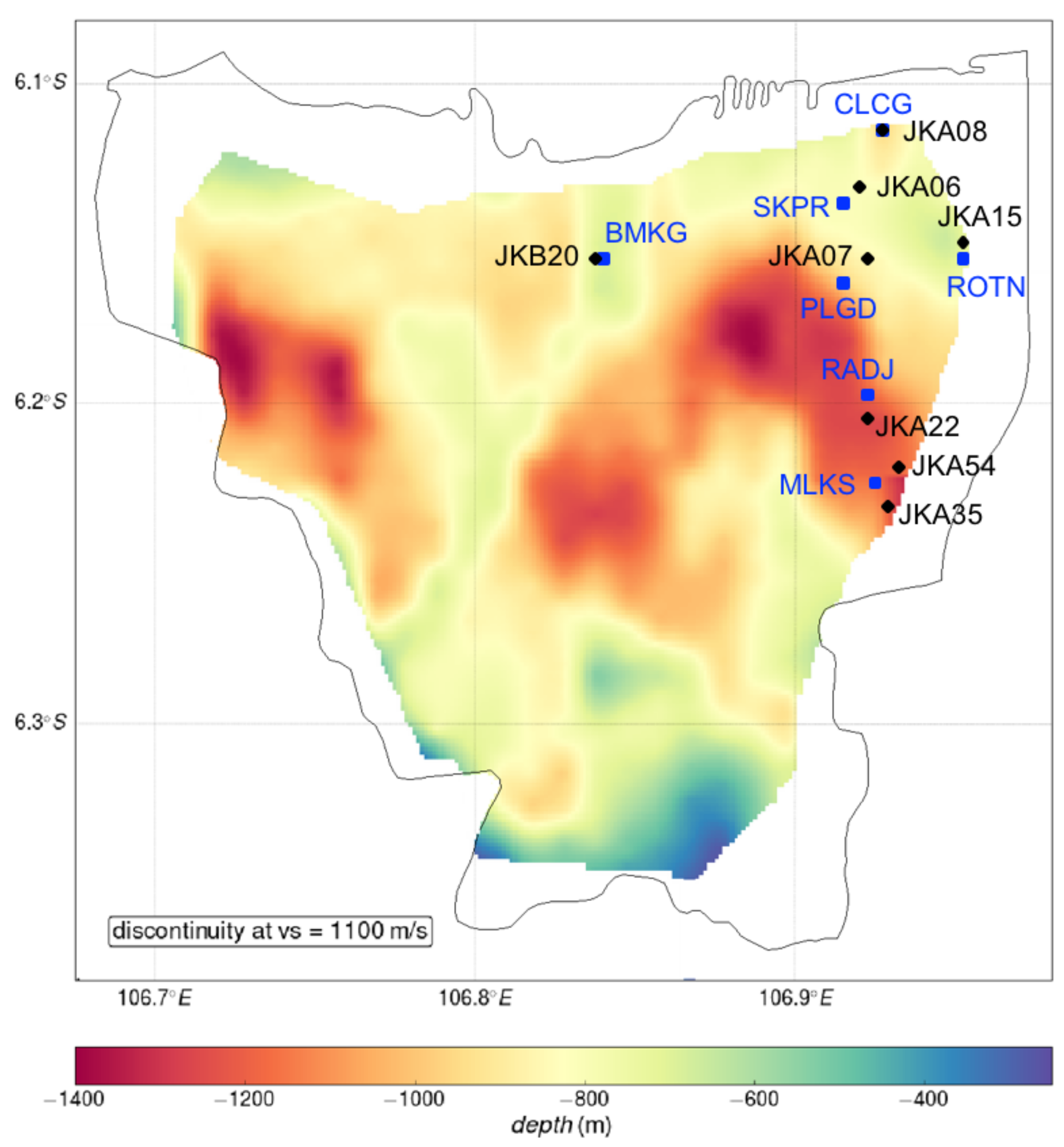
3. The Jakarta Basin

A model of the seismic velocity structure of the Jakarta Basin was constructed by Cipta et al. [13] using analysis of Horizontal-to-Vertical Spectral Ratios (HVSR) of ambient seismic noise (Figure 2), but this model does not extend to the basin edges. The sediment deposits along the city border are thick, from about 200 m in the south, to 800 m in the west and more than 1000 m in the east. Because the model does not include the basin edges, it is necessary to extend the model beyond Jakarta itself to estimated plausible margins of the basin, which are presumed to be the axes of low angle folds that will appear as topographic highs. For this purpose, geological data namely, the lateral distribution of lithology, drainage pattern and topographic information was utilized. A simple method to reconstruct the paleo-topography called the arc-method is used (for detail see e.g., Allmendinger [31]). By comparing geological data and sediment thickness as presented in Figure 2, it is a reasonable guess to interpret the basement of the basin as the upper Parigi formation deposited in the Late Miocene. To construct a paleotopography, i.e., a topography before the more recent Cibuluh formation was deposited, we need to plot the strike and dip of the Parigi formation layering in a 2D cross-section.

The topographic map shows that Jakarta in particular and the north coast of West Java in general is an area of gentle slope (slope 1–10 %). The morphology and surface lithology of this area is well illustrated in its drainage pattern, an excellent example of a dendritic drainage pattern characteristic of gentle topography with homogeneous lithology. Careful analysis of the drainage pattern discloses the faint topographic highs to the west and east of the city. Most of the tributaries of the Cisadane River (1 In Figure 3) flow only from the west, while further to the west the Cimanceuri River (4 in Figure 3) flows from the south, veers westward then flows northward. These two rivers encircle a topographic high that can be identified with the western rim of the Jakarta basin. The geological map shows that near the Cimanceuri River (4 In Figure 3) the lithology is changing from aluvial fan Qav to QT tuff (north) and Oligocene-Miocene formations (south). This changing lithology confirms the hypothesis that the Cimanceuri River lies at the western rim of the Jakarta basin, in the slightly elevated land that is known as the Tangerang High.

The Kali Bekasi River (3 in Figure 3) to the east of the city receives water intake mostly from the east, and further to the east the Citarum River (5 in Figure 3) flows from the south, turns to the east and circles back to the west, eventually flowing into the Kali Bekasi River and the Java Sea. This drainage pattern is indicative of a topographic high just east of the Kali Bekasi River, known as the Rengasdengklok High.

The Kali Bekasi River also marks the boundary between two alluvial fan bodies, alluvial fan Qav to the west of the Kali Bekasi River, and alluvial fan Qav/Qos to the east of the river. The changing lithology and topographic high to the east suggest that the eastern rim of the basin is situated around the Kali Bekasi River.

Oil prospecting studies using the seismic reflection method have succesfully recognized five principal oil reservoir groups within the North West-Java Basin. These oil caps are (1) Eocene–Oligocene fractured volcanics (Jatibarang Volcanics), (2) Oligocene–Lower Miocene deltaic sandstones (Talang Akar Formation), (3) Lower Miocene reefs (Baturaja Formation), (4) Lower–Middle Miocene sandstones (Upper Cibulakan Formation), and (5) Middle-Upper Miocene carbonates (Parigi Limestones and Upper Cibulakan Formation) (Kingston [32]). On the top of these reservoirs, the Parigi, Cibuluh and Quaternary formations were deposited successively, with a hiatus due to decreasing sea level separating these formations. From these data, it can be inferred that the Jakarta Basin, also known as the Ciputat Basin, is part of the North West-Java Basin in which the basement is composed of carbonates of the the upper Parigi formation deposited in the Middle-Upper Miocene (see Figure 6 in Putra et al. [33]).

The arc method, also known as the Busk method (named after H. G. Busk and nicely explained in Allmendinger [31]), is used to reconstruct the carbonates of the Parigi Formation, so that the basin basement extends outside the area in which it is inferred from the HVSR measurements. In using the arc method, it is assumed that the stratigraphy of the Parigi formation has not been strongly affected by erosion. The final basin model, which is the composite of the HVSR-derived model (covering the city) and that derived using the arc method (covering outside the city to the basin’s rim) is presented in Figure 4.

4. Material and Methods

4.1. Ground Motion Prediction Equations (GMPEs)

A GMPE is a generic term for a mathematical relationship between a statistical estimate of expected ground motion, and earthquake magnitude and some measure of distance to the earthquake fault rupture. GMPEs can supply a probability density function of ground motion values for a given earthquake scenario. These equations provide probabilistic descriptions of the level of ground shaking as a function of the earthquake parameters, accounting for path and site effects. Some Next Generation Attenuation (NGA) functions take into account independent estimator variables such as earthquake magnitude ($f_{mag}$), geometric attenuation ($f_{dis}$), style of faulting($f_{flt}$), hanging-wall geometry ($f_{hng}$), shallow site response ($f_{site}$), basin response ($f_{sed}$), hypocentral depth ($f_{hyp}$), rupture dip ($f_{dip}$), and (apparent) anelastic attenuation ($f_{atn}$) (Campbell & Bozorgnia [34]). They model a ground motion parameter Y, which could represent Peak Ground Acceleration (PGA), Peak Ground Velocity (PGV) or spectral acceleration (SA) at specific periods as:

$$lnY=f_{mag}+f_{dis}+f_{flt}+f_{hng}+f_{site}+f_{sed}+f_{hyp}+f_{dip}+f_{atn}$$

(1)

Out of these parameters, we are interested in investigating the $f_{sed}$ parameter, which is intended to parametrize basin depth. The preliminary ground motion simulations are readily performed as the selected NGA GMPEs (CY2014 and CB2014) are incorporated in OpenQuake, a software platform developed by the Global Earthquake Model (GEM) Foundation for seismic hazard and risk calculations Pagani et al. [35].

The three GMPEs mentioned above require site parameters that use $V_{S30}$ as a proxy for near-surface geology (soil) classification, and $Z_{1.0}$ or $Z_{2.5}$ to describe basin depth ($Z_{1.0}$ is the depth to a $V_S$ of 1 km/s, while $Z_{2.5}$ is depth to 2.5 km/s). Using data from Japan and California, Chiou & Youngs [8] provide empirical equations relating $V_{S30}$ and $Z_{1.0}$ and Campbell & Bozorgnia [34] provide empirical equations to estimate $Z_{2.5}$. To asses whether the velocity structure of the Jakarta Basin covers a similar parameter range to those in California and Japan that are used for these GMPEs, we plotted the empirical equations of Chiou & Youngs [8] for $Z_{1.0}$ as a function of $V_{S30}$ against data from the Cipta et al. [13] model for the Jakarta Basin, where $Z_{1.0}$ is taken directly from the model and $V_{S30}$ is either taken from the Cipta et al. [13] model or the NSPT data of Ridwan [36].

Regardless of which estimate of $V_{S30}$ is used, Figure 5a shows that $Z_{1.0}$ estimated for the Jakarta Basin are always much greater than the $Z_{1.0}$ calculated from the Chiou & Youngs [8] empirical relations, either for California or Japan. Figure 5b shows amplification of PSA as a function of period for $V_{S30}$ = 100 m/s, typical of the Jakarta Basin, and values of $Z_{1.0}$ ranging from 100 to 1500 m. The amplification curve for $Z_{1.0}$ = 100 m exhibits a pronounced peak at period 0.8 s, and this peak broadens and its period increases to 1.5 s and 2.0–2.5 s for $Z_{1.0}$ = 500 and 1000 m, respectively, but changes little in amplitude or period range for $Z_{1.0}$ = 1500 m. A typical HVSR curve for the Jakarta Basin, on the other hand, exhibits a pronounced peak at around 6 s (some curves such as this one also exhibit a secondary peak at shorter periods, see Cipta et al. [13]. While the HVSR curve does not necessarily represent the amplification of seismic waves, its peak period is widely regarded as coinciding with that of S-wave amplification Nakamura [37], it has been used to explain spatial patterns of earthquake damage Gosar [38], and it agrees with the fundamental period of S-wave resonant oscillation calculated form the Jakarta Basin velocity models of both Cipta et al. [13] and Saygin et al [39]. Thus, the basin parameters calculated for the Jakarta Basin model of Cipta et al. [13], appear to lie outside the range of values used for the development of the deep sediment corrections of CY2014, and the period dependence of CY2014 predictions for PSA using these corrections do not agree with the characteristics of ground motion implied by observed HVSR curves. Therefore, Therefore, we are skeptical that the deep sediment corrections of CY2014 will correctly account for seismic resonance in the Jakarta Basin.

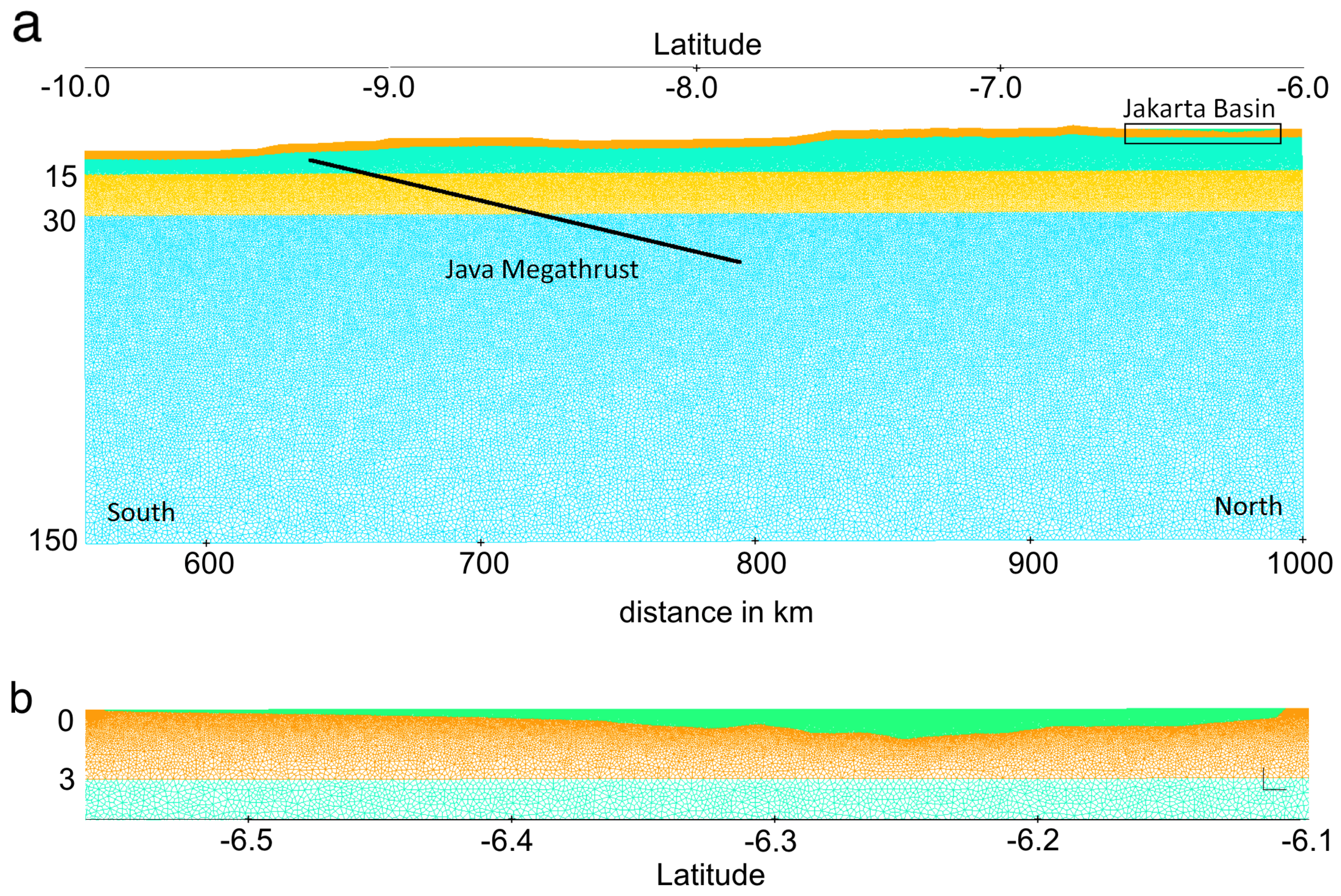
4.2. Numerical Simulation of Seismic Waves

Earthquake-generated ground shaking depends not only on the earthquake source parameters, but also on the medium in which seismic waves propagate, especially near surface and basin structure. In this study, seismic waves generated by synthetic ruptures on a crustal fault, the Java Megathrust, and an intraslab fault are simulated using SPECFEM2D. This software uses the Spectral Element Method (SEM), which combines the flexibility of the finite element method (FEM) with the accuracy of high-order (trigonometric) element basis functions. SEM is very effective at achieving high accuracy even for realistic earth models, and is therefore applicable for a wide range of applications in seismology (Komatitsch & Vilotte [16]). This approach to scenario ground modelling is similar to that used by Molnar et al. [40] and [41] to study seismic wave interaction with 3D structure of the Georgia Basin, British Columbia, Canada.

The seismic characteristics of the Jakarta Basin as obtained from the HVSR analysis will be represented in our 2D domain as a SN cross section over which the earthquake simulation takes place. To avoid extremely small elements, the sediment inside the basin is taken to be a homogeneous medium overlying bedrock, which is part of a 3-layer lithosphere, with maximum domain area as large as 445 km in length by 150 km in depth (Figure 6). The shear-wave velocity both in the sediment-filled basin and bedrock are taken as averages from the corresponding depths of the HVSR model. Crustal P-wave velocity ($V_P$) outside the basin is taken to be 1.8 times $V_S$ as indicated in Cipta et al. [13].

The surface geology in the area of interest, from older to younger deposits, is composed of Tertiary marine formations, Pliocene-Pleistocene volcanic rocks, alluvial fan and recent alluvium. Alluvial fan deposits are the main component filling the basin, overlaying the Tertiary-Quaternary volcanic rocks that are presumed to act as basement. It is also possible that Miocene marine deposits play a role as bedrock, especially in the northern part of the basin. Heterogeneities both in vertical and horizontal directions make it difficult to set the elastic properties of the basin, particularly since the very low $V_S$(<100 m/s) near the surface will require extremely small elements to model accurately. Instead of describing the detailed spatial variation of basin velocities, $V_S$ is set to the average velocity in the basin resulting from inversion of HVSR ellipticity curves, 582m/s. Compressional-wave velocity ($V_P$) in the basin is set to 3–4 times $V_S$ under the assumption that as a groundwater basin, the sediments filling Jakarta Basin are highly saturated, as also indicated by HVSR inversion that shows high (∼4) $V_P/V_S$ (Cipta et al. [13]).

The total length of the computational domain for the megathrust event extends from 6° to 10° south latitude, the maximum depth is 150 km and highest elevation is 1.5 km. The topographic surface is extracted from the Shuttle Radar Topography Mission DEM (SRTM Digital Elevation Model, freely downloaded from: https://dds.cr.usgs.gov/srtm/ version2_1/SRTM3/Eurasia/). The domain area accommodates source locations and is divided into 5 zones including the basin, a 3-layer crust and the mantle. Irregular quadrangle meshes are generated to fill the domain area, the coarsest (maximum gridsize: 2000 m) meshes filling the lower layer while the finest meshes are arranged in the basin (maximum gridsize: 12.5 m). The very small mesh size in the basin, together with the large computational domain that includes the megathrust, results in a very large mesh size, of 800,000 elements. This large mesh size is the main reason that calculations in this study were limited to 2-D, as a 3-D mesh at this resolution would have resulted in very long computation time. The topographic surface is set to be a free surface while the other sides are set to be absorbent surfaces to avoid waves reflecting back into the domain area (see Figure 6).

While seismic attenuation in sedimentary basins like Jakarta can be high, we found that the viscoelastic calculations of SPECFEM2D for our large computational mesh were prohibitive (even the elastic calculations using 28 CPUs required a wall time of 18 hours; viscoelastic calculations took much longer). To our knowledge no studies of seismic attenuation or seismic quality factor for the Jakarta region have been undertaken, but in order to test the influence of attenuation we use Qp = 44 and Qs = 25, taken from a study conducted Hauksson et al. [42] in the Los Angeles Basin. Tests using these values for Qp and Qs in the basin indicated that viscoelasticity had a small effect for periods > 1 s. Therefore, in the simulations described here we neglected attenuation in the basin for reasons of computational efficiency. All parameters for simulations are presented in

Table 1. Domain parameters used in simulation.

Layer	Rho	${\mathit{V}}_{\mathit{P}}$	${\mathit{V}}_{\mathit{S}}$	${\mathbf{Q}}_{\mathit{\kappa }}^{\mathbf{*}}$	${\mathbf{Q}}_{\mathit{\mu }}^{\mathbf{*}}$	Max Depth
	(kg m−3)	(ms−1)	(m−1)			(m)
Basin	1200	1600	582	44	25	1385
Layer 2	2200	4100	2300	283	150	3000
Layer 3	2900	5100	2800	450	450	13,467
Layer 4	3200	6500	3200	500	500	15,000
Layer 5	3800	8000	4000	600	700	120,000

* Parameter values were tested but not used in the simulations presented here.

.

In this study, we assume that seismic waves are generated outside the basin, in the Java subduction zone for the megathrust scenario, in the shallow crust to the south of the basin for the crustal earthquake scenario, and in the mantle for the intralsab scenario. Seismic waves propagate from the source through a 5-layer mantle + crustal model to the surface, as indicated in Table 1 On the surface, both inside and outside the basin, seismic waves will be recorded at stations located at 2 km spacing along a south-north cross-section. In order to account for 3-D geometrical spreading and attenuation in the crust and upper mantle outside 2-D elastic simulation, we scaled the computational results by matching the long-period (1–10 s) spectra of seismograms recorded just outside the basin with results from suitable GMPEs for the appropriate magnitude and distance. For the megathrust scenario, we scaled the seismograms by matching spectra with results of the AEA2014 GMPE, for the crustal source we used CY2014, and for the intraslab earthquake scenario we matched spectra to AEA2014S.

5. Results

5.1. GMPE Modeling Results

GMPE simulations have been performed for the three earthquake scenarios described above and results for the crustal earthquake scenario are displayed in Figure 7. Figure 7a–c show amplification of PGV, PGA and PSA(5 s) which vary between 200–500, 70–180 and 200–700%, respectively (note that we describe amplification following Pilz et al. [43], as described below in Section 6.2, where 0% corresponds to hard rock ground motion). The absolute values of these quantities are shown in Figure 7e–g, where it can be seen that PGV, PGA and PSA(5 s) have values of about 6 cm/s, 5% g and 0.6–0.8% g near the southern edge of the basin, about 60 km from the earthquake source. As distance from the earthquake increases in the center and northern part of the basin, the absolute level of ground motion (Figure 7e–f steadily decreases with increasing distance from the earthquakes. The amplification (Figure 7a–c), on the other hand, increases in the north of the basin, closely following the pattern of $V_{S30}$ decrease indicated in Figure 7d.

For the amplification at PSA (5.0 s), which is close to the apparent resonance peak in most of the HVSR measured by Cipta et al. [13], it might be expected that variation in basin geometry would have a significant influence on the long period ground motion, but there is very little correlation with the pattern of basin depth variations (Figure 7h). We believe this is reflective of the “saturation” in peak ground motion period depicted in Figure 5a as $Z_{1.0}$ reaches the value 1000 m that is typical of most of the Jakarta Basin. For this reason, it seems clear that caution should be used when trying to use the deep sediment terms of CY2014, and presumably othe GMPEs with deep sediment correction developed using similar datasets, to describe basins elsewhere, to estimate earthquake ground motion in the Jakarta Basin.

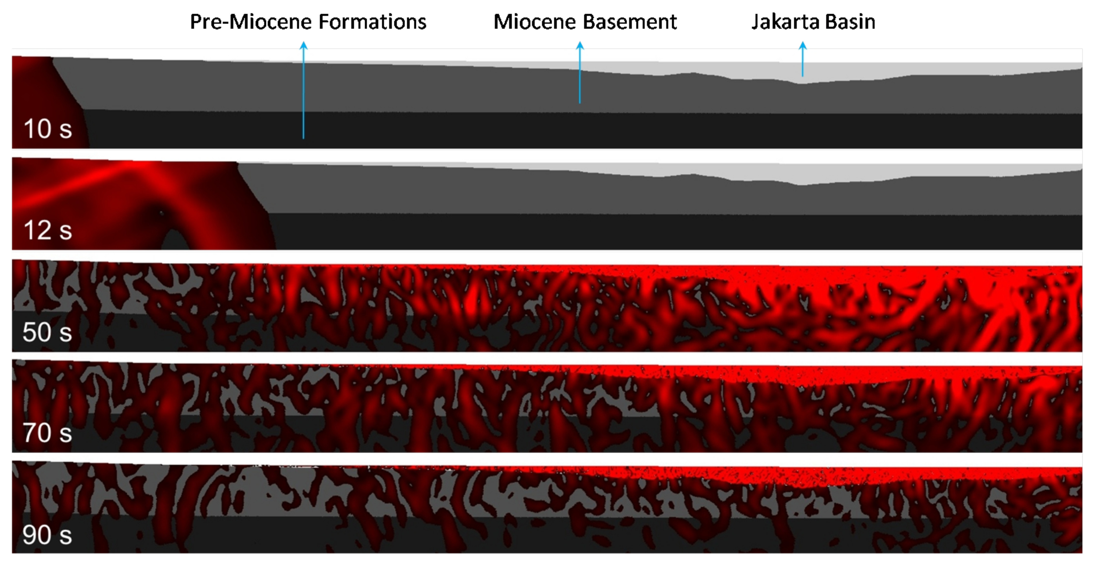
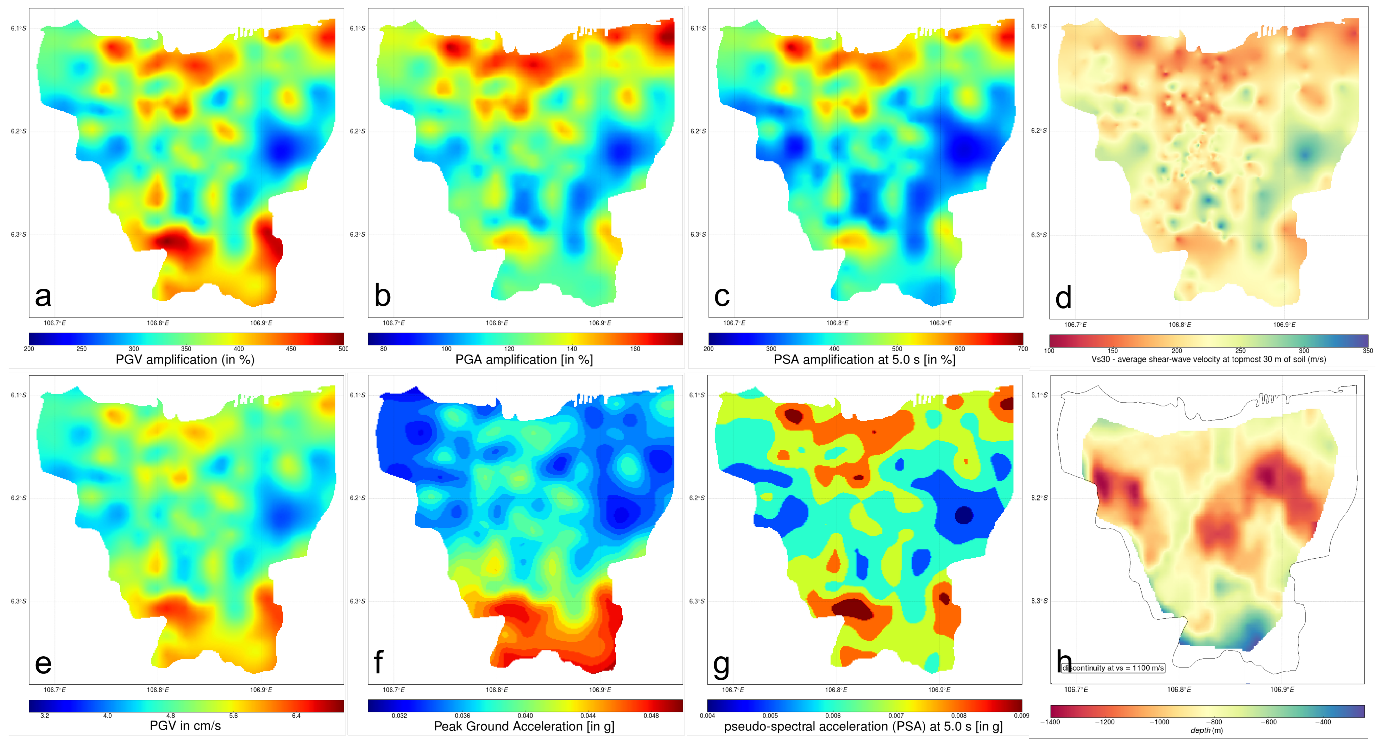
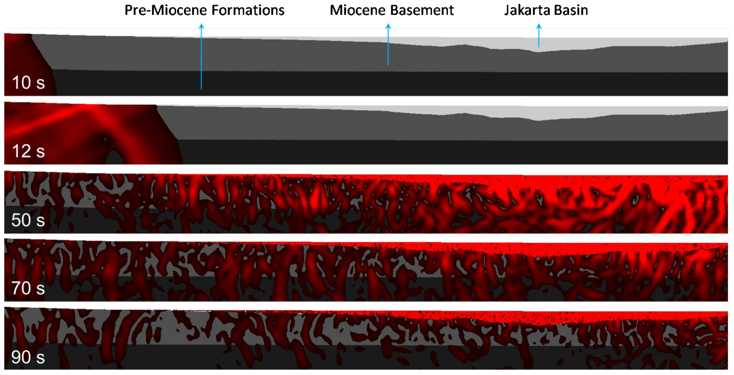
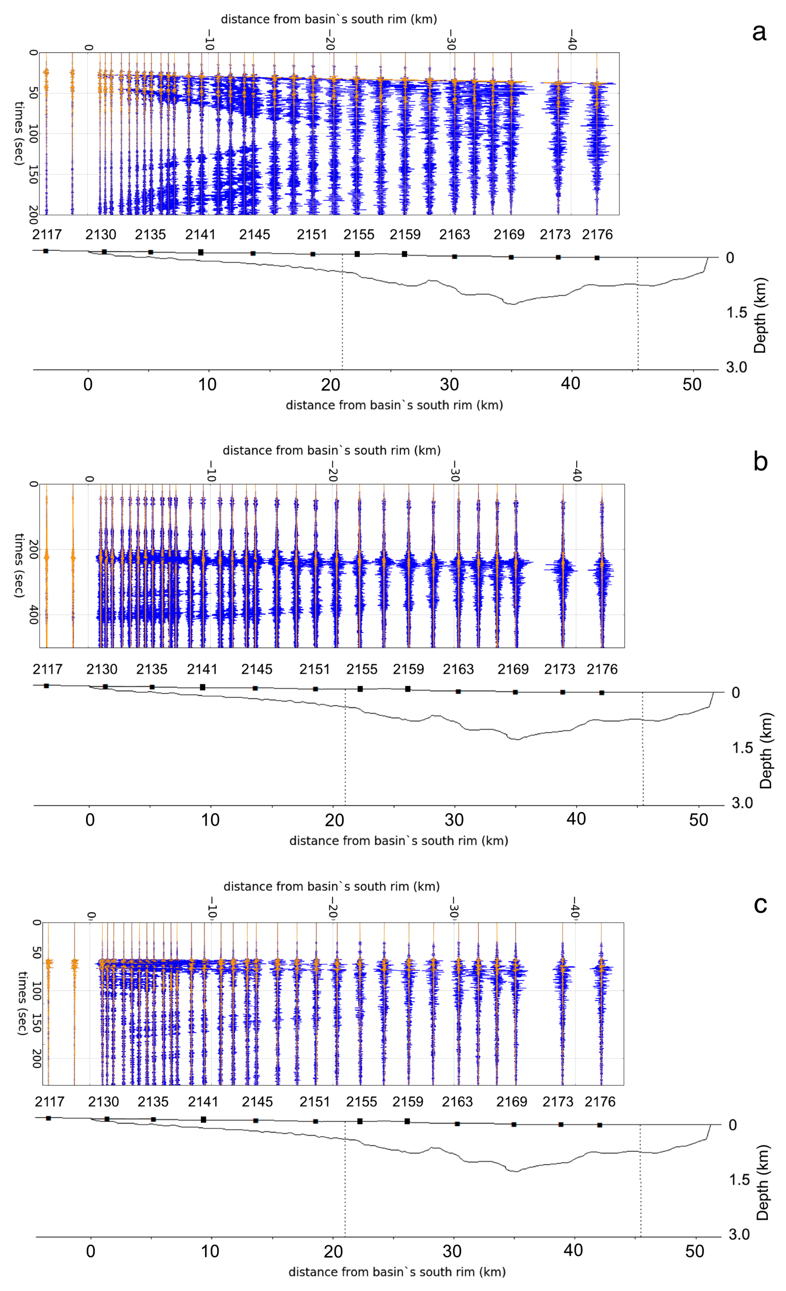
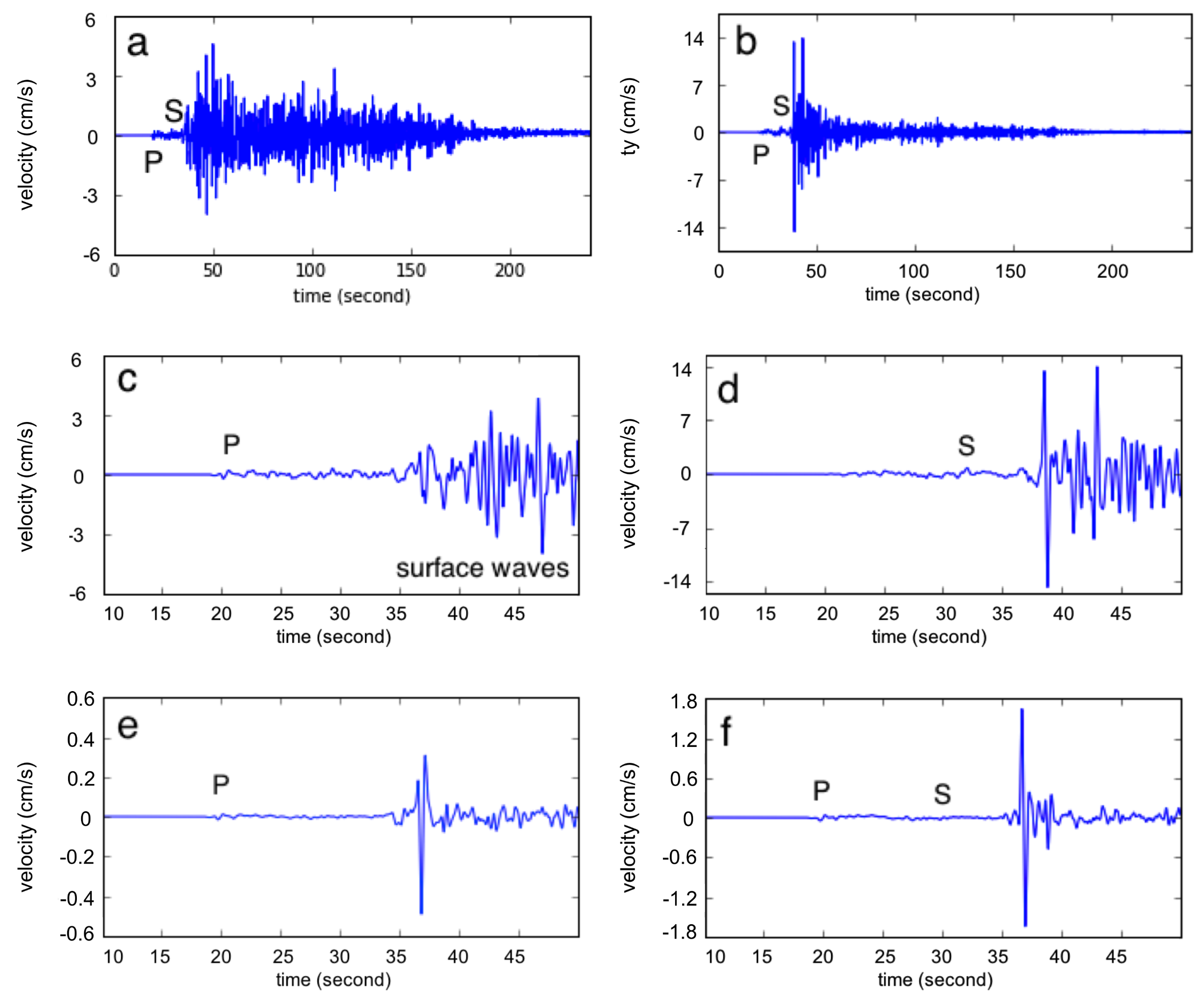
5.2. Numerical Simulation Results

The crustal and megathrust events are situated south of Jakarta at distances 85 km and 200 km and with magnitudes $M_w$ 6.5 and $M_w$ 9.0, respectively. The megathrust is dipping north while the crustal fault is dipping south. The third scenario simulates propagation of seismic waves originating from a medium-depth intraslab earthquake located at the depth of the subducting slab at 180–204 km (fault width = 34 km) directly beneath the city. This fault is dipping south and the earthquake has magnitude $M_w$ 7.0.

Snapshots from the crustal fault scenario are presented in Figure 8. After 10 s, the P-wave is showing up in the lower left corner of the topmost panel and at 12 s, both P-wave (dark) and S-wave (vermilion) are observed approaching the basin. At 50 s, seismic waves, both body and surface waves, have entered and are trapped inside the basin. Surface waves are modulated inside the basin and at 90 s, while body waves are attenuated and have faded away outside the basin, surface waves are still reverberating in the basin.

Seismograms (horizontal component) resulting from these three scenarios are presented in Figure 9a–c. Two types of seismograms are plotted: (1) those calculated using the elastic parameters indicated in Table 1, colored blue in Figure 9 and referred to here as ’basin seismograms’, and those calculated using an identical computational mesh but with the basin elastic parameters replaced by those of the basement (i.e., the Basin parameters in Table 1 are replaced by those of Layer 2), colored orange in Figure 9 and referred to here as ’bedrock seismograms’. The three record sections in Figure 9a–c clearly show that seismic waves propagating through the soft sediment inside the basin are amplified to different degrees. Outside the basin the orange colored curves (bedrock seismograms) match the blue curves (basin seismograms) perfectly, meaning that outside the basin, no amplification is observed. On the other hand, inside the basin, basin seismograms have much higher amplitudes and prolonged durations in comparison to bedrock seismograms. It is interesting to note that the basin-bedrock seismogram ratio is not uniform, and basin depth is not the only factor contributing to the amplification. Basin geometry and direction of incoming waves also appear to influence the degree of amplification.

For the crustal earthquake scenario, Figure 9a, seismic waves propagating toward the north edge of the basin are reflected back into the basin and recorded at 200 s at the southernmost station (S2117) and at progressively earlier times at more northerly stations. However, at S2157 to S2176, reflected waves are not clearly seen because they interfere with seismic waves propagate northward, producing high amplitude seismograms at 50–60 s (Figure 14). The megathrust earthquake also exhibits reflected waves that are clearly observed at S2130 to S2169, again with reflected waves recorded earlier in the north than in the south (Figure 9b).

In contrast to the other two scenarios, the intraslab earthquake scenario shows reflected waves from both south and north edges. Near the south edge, high amplitude seismic waves are observed at stations S2130-2135 at times 50–100 s. These high amplitudes are generated from interaction between incoming and reflected waves as well as trapping at the basin’s edge. As time goes by, waves reflected by the northern edge of the basin are recorded after 100 s in the southern stations and recorded earlier in the central and northern stations.

Seismograms in Figure 10a,b record incoming P- and S-waves at 20 s and 36 s, respectively, for the crustal fault scenario. For the basin seismograms in Figure 10c,d, the direct S-wave is followed by a series of reverberations comprised of S-wave and Rayleigh wave energy, that builds up over the following 15 s, with the highest vertical component amplitude achieved 10 s after the direct S-wave arrival. It is observed that S-wave/Rayleigh wave coda that builds up at about 37 s is still observed after more than 150 s. The bedrock seismograms (Figure 10e,f) are dominated by the direct S-wave and have a very weak coda after only a few seconds.The long duration (>120 s) and very high amplitude of basin seismic waves after 40 s is likely due to the constructive interference between seismic body waves and surface waves.

The intraslab scenario produces similar results, at the same station, with surface waves observed after 55 s and still trapped inside the basin after 240 s. In the case of the megathrust event, the Rayleigh wave arrives about 25 s after the P-waves recorded in the seismograms. The interference of reverberating surface waves leads to very high amplitudes, compared to the crustal and intraslab scenario. Entrapment of seismic waves inside the basin prolongs the duration of seismic waves, with high amplitude seismic waves still observed 10 minutes after the earthquake. Interference between seismic body waves and secondary surface waves was recognized as a main cause of building collapse in Kobe during the 1995 Great Hanshin Earthquake (Zhao et al. [44]).

The three scenarios indicate that the larger the magnitude, the longer the seismic waves were observed inside the basin. The “red” (i.e., long-period dominant) spectra of frequency content generated by the larger rupture area may be responsible for the very long duration of long period ground motions generated by the megathrust scenario. Together with the maximum amplitude and duration of seismic waves, frequency content is also a very important factor that is responsible for building damage. According to Shoji et al. [45], duration is more event-dependent than site-dependent while the site-dependency for a given total power is greater than the event-dependency.

6. Discussion

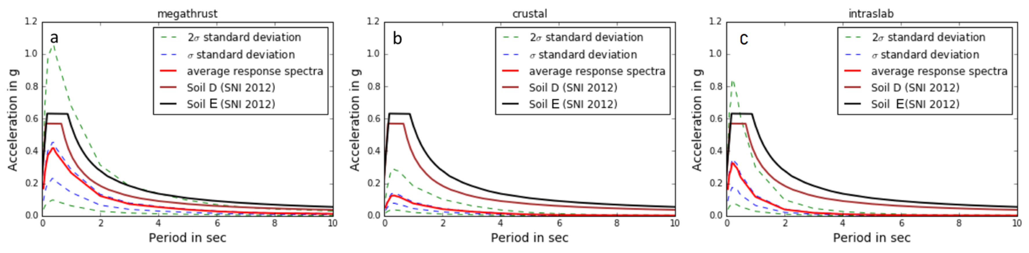
6.1. GMPE-Seismic Hazard

Using GMPE modelling, pseudo-spectral acceleration (PSA) for each spectral period can be computed, and it’s variability can be accounted for by sampling the aleatory variability in the GMPEs as well as computing ground motion over the range of site response information ($V_{S30}$ , $Z_{1.0}$, and $Z_{2.5}$) available for the Jakarta Basin. Results for average and 1- and 2-$\sigma$ simulated response spectra (SRS) for the three earthquake scenarios considered are shown in Figure 11, where they are compared with the design response spectra for Jakarta. At short periods (< 1 s), the average and 1-$\sigma$ simulated response spectra (SRS) curves lie well below the design spectra for all three scenarios, but the 2-$\sigma$ curves exceed the design spectra for the megathrust and intraslab scenarios. However, since GMPE simulations do not fully take the effects of basin geometry into account, longer period PSA may be underestimated, and hence we need to be careful in interpreting the curves presented in Figure 11. For this reason, let us compare design seismic response and SRS at the shorter periods (<1 s) only, and note that shorter period response spectra correspond to the natural resonance of most residential buildings (which, however, are not generally required to conform to the Indonesian building code).

The current building code (2012 Indonesia’s National Standard–SNI 1726-2012) adopted the updated seismic map of Irsyam et al. [46] that estimated ground motions for a 2% probability of exceedance in 50 years (2500 years return period) as the maximum considered earthquake (MCE) level. Figure 11 shows that the current seismic building code in Indonesia that takes into account D and E soil classes performs well against the PSA estimated from GMPEs for the crustal earthquake scenario, but has significant probability of being exceeded (at the 2-$\sigma$ level) for the megathrust and intraslab earthquakes. In this figure, the thick black and magenta curves represent designed ground motion produced by the MCE in a 2500 years return period for D- and E-type soils, respectively.

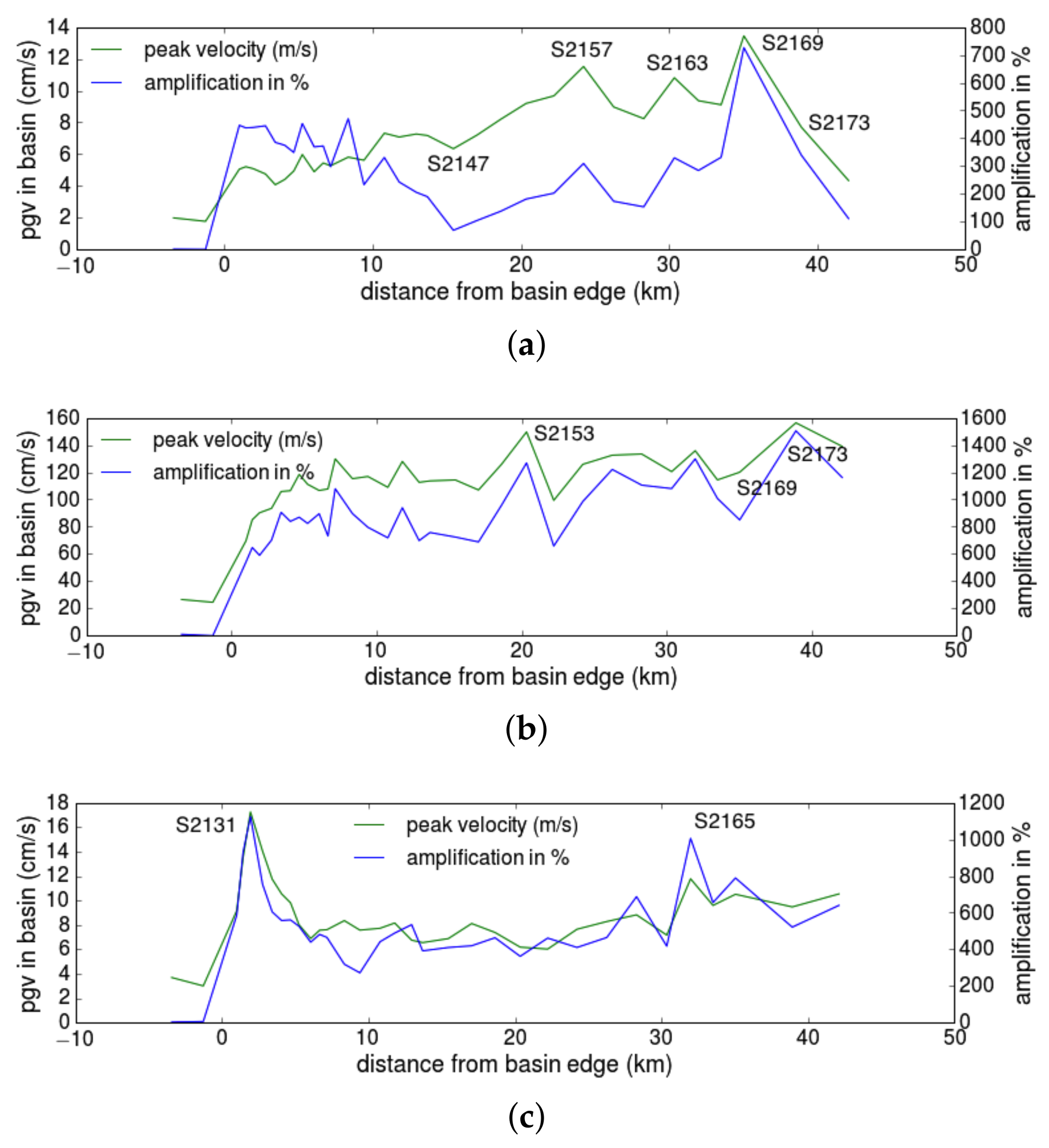
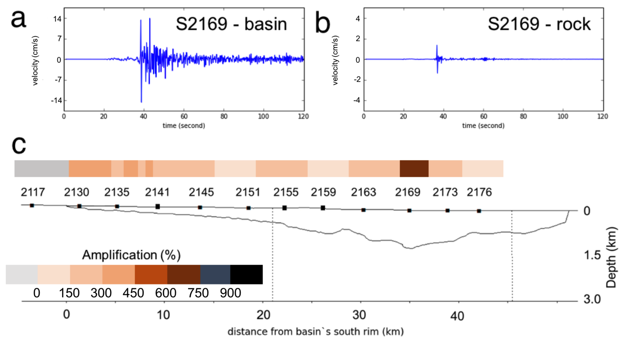
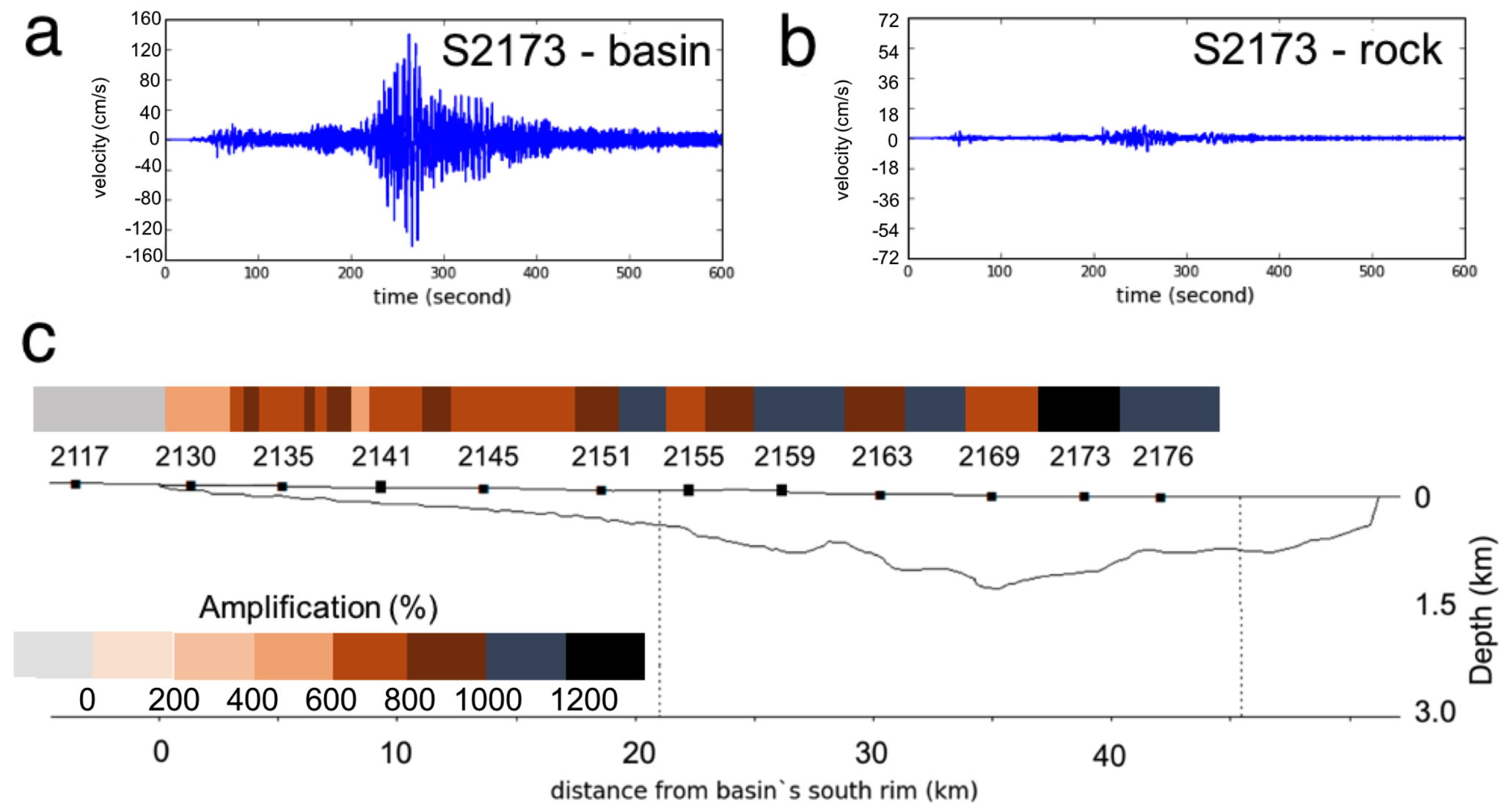
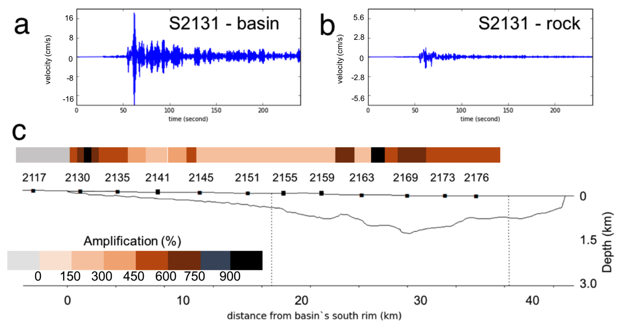
6.2. Numerical Simulations–Peak Ground Velocity (PGV)

The Mw 6.5 crustal fault scenario generates a maximum peak ground velocity of 13.45 cm/s and the maximum PGV amplification is about 726%. Figure 12a shows that amplification is not uniform throughout the basin, while in S2147 basin depth gives small effect to peak velocity, in other stations basin geometry amplify peak velocity significantly. Most striking is the amplification observed at S2169 at the deepest part of the basin (Figure 12 and Figure 13a–c. Amplification here is describe in a manner similar to that used by Pilz et al. [43] in calculating estimated PGV amplification in Santiago Basin, Chile: we subtract the PGV values for the bedrock seismograms from the value for the basin seismograms, and divide this by the PGV value for the bedrock seismograms (multiplying by 100 to convert to percentage amplification).

Different characteristic of simulated PGV and amplification are produced by megathrust earthquake scenario. PGV and amplification tent to incerase as the basin gets deeper. Prominent high PGV and amplification are simulated at stations S2153 and S2173. Simulated PGV at these stations are 149.67 cm/s and 153.37 cm/s while amplifications are 1269% and 1504%, respectively (Figure 12a and Figure 14a–c). While these ground motion levels may seem very high, we note that the $M_w$ 9.0 Tohoku Earthquake resulted in 50 cm/s pseudo-velocity response at 7 s period observed in the Osaka Basin at 770 km distance, along with 2.7 m peak-to-peak roof displacements at one high-rise building (Sato et al. [47] and Tsai et al. [48], respectively). The $M_w$ 8.0 Michoacan earthquake resulted in an observed PGV of 40 cm/s at 350 km distance (Singh & Ordaz [49]). In light of these observed basin effects observed at much greater distance and smaller magnitud, our simulated result of ≈150 cm/s for a $M_w$ 9.0 earthquake at 250 km distance from Jakarta Basin does not seem unreasonable.

The intraslab earthquake scenario results in very large amplification, especially at S2131 (1134%), so that the estimated PGV in that station (17.24 cm/s) is significantly higher than the other stations. The source of the intraslab scenario is very deep and directly beneath the city, so that rupture-to-station distance is the same for all stations, hence the variation of amplification with respect to rupture distance can be neglected. Therefore, large amplification at this station is most probably due to focusing of seismic waves by the basin edge, while trapping of seismic waves inside the basin may also affect amplification at this station. High amplification is also recorded at S2165, where particulary thick basin fill is responsible for large amplification (Figure 12a and Figure 15a–c). Recorded PGVs (cm/s) and amplification (%) for all three scenarios are presented in

Table 2. PGVs and Amplification in % resulted from 3 scenarios.

Station	PGV-C	Ampli-C	PGV-M	Ampli-M	PGV-S	Ampli-S
Station	(cm/s)	(%)	(cm/s)	(%)	(cm/s)	(%)
S2117	1.98	1	26.44	8	3.68	2
S2124	1.77	0	24.39	−2	3	5
S2129	5.05	447	69.49	539	9.15	586
S2130	5.21	437	85.07	646	13.52	930
S2131	5.08	439	90.2	589	17.24	1125
S2132	4.75	445	93.46	701	14.03	754
S2133	4.07	385	105.82	906	11.74	604
S2134	4.4	375	106.43	838	10.54	557
S2135	4.94	349	118.45	869	9.8	560
S2136	5.98	453	111.16	824	8	525
S2137	4.89	369	106.6	895	6.88	439
S2138	5.44	372	107.74	731	7.56	481
S2139	5.27	297	129.84	1079	7.6	465
S2140	5.81	470	115.27	896	8.34	318
S2141	5.62	233	116.89	795	7.56	271
S2142	7.32	331	108.93	718	7.72	441
S2143	7.08	242	127.94	939	8.15	488
S2144	7.27	205	112.59	697	6.74	534
S2145	7.17	190	113.63	757	6.54	391
S2147	6.34	69	114.33	723	6.87	409
S2149	7.2	104	106.95	688	8.11	419
S2151	8.19	137	125.93	959	7.37	463
S2153	9.19	181	149.67	1269	6.17	361
S2155	9.67	202	99.34	657	6.01	461
S2157	11.52	309	125.83	985	7.64	410
S2159	8.97	173	132.54	1221	8.27	464
S2161	8.23	153	133.4	1105	8.82	687
S2163	10.81	330	120.44	1080	7.16	417
S2165	9.36	284	135.84	1298	11.77	1005
S2167	9.11	331	114.37	1007	9.59	655
S2169	13.45	726	120.02	849	10.5	789
S2173	7.7	339	156.37	1505	9.47	521
S2176	4.34	111	139.01	1162	10.53	640

PGV-C, PGV-M, PGV-S, Ampli-C, Ampli-M, Ampli-S are peak ground velocity (PGV) and amplification (Amp) generated from crustal fault, megathrust and intraslab.

. Minor amplification or deamplification recorded at stations S2117 and S2124 that are located outside the basin may come from simulation noise.

6.3. Numerical Simulation-Response Spectral Acceleration

The megathrust scenario generated the highest peak ground velocity and amplification in the basin, especially at station S2173. In this section, we will look at the response spectral acceleration that is widely used to characterise ground motion in civil engineering, then compare the design building code against spectral acceleration resulting from SPEFEM2D modeling. At station S2169 and S2173, simulated horizontal acceleration at period 1 s are about 0.45 g, which is higher than the design response spectra used by the building code. At periods about 1 s very high accelerations are observed (Figure 16a,c), however, these results may be inaccurate since neither near surface attenuation $\kappa$ nor crustal and basin frequency-dependent attenuations for $V_P$ and $V_S$ (Qp and Qs) for Jakarta region are available.

Since long period (>3 s) ground motions are much less sensitive to $\kappa$, Qp and Qs, it seems reasonable to consider how these compare to the design response spectra. At S2169, for all frequencies, mean ground motion predicted from GMPE fall below both the 2012-SNI Irsyam et al. [46] in Figure 11 and the 2002-SNI Puskim [50] (see also Sukamta & Alexander [51]) design response spectra (Figure 16a–d). On the other hand, ground motion predictions on soil inferred from the SPECFEM2D modeling are much higher than design response spectra of 2002-SNI (since 2012-SNI provides response spectra from PGA to PSA 4 s, we compare PSA 4–10 s with 2002- SNI). Figure 16a–d shows that ground motion on bedrock is lower than 2002-SNI and 2012-SNI, therefore we believe that basin depth and surface condition is of great importance for magnifying seismic motion, as shown in Figure 12b and Figure 14a–c amplification factor can reach 1200% for megathrust events. This amplification factor should be considered.

For the intraslab earthquake scenario, basin edge effects can be particularly pronounced as observed in Figure 9c. Amplification of short period ground motions, particularly at periods of about 1.0 s, result in very high acceleration (>1 g) at S2131 (Figure 17). At this point, the PGV amplification is 1125% (Figure 15 and Table 2), but this high frequency content may not be realistic due to the lack of consideration of attenuation effects as discussed above. On the other hand, large amplification at S2165 in the deepest part of the basin as can be seen in Figure 12c and Figure 17 is experienced by ground motion at period >4. The spectral amplification at this point is as high as 424%. There is interesting characteristic of amplification at S2131 and S2165, while PSA >4 s at S2131 fall below the 2002-SNI design response spectra (Figure 17b) , at S2165 the scenario response spectra at about 5.5 s is much higher the design response spectra (Figure 17b). An acceleration of about 0.2 g and amplification of 335% (for period of 5.5 s) are estimated by the simulation (Figure 17).

7. Conclusions

We have shown that GMPE modeling predicts significant influence of near-surface geology, represented by $V_{S30}$ , on short-period (<1 s) seismic waves. However, for a very deep basin filled with soft sediment, available GMPEs are not capable of capturing the effects of basin geometry on seismic waves, at least for basins the Jakarta Basin. Consequently, more realistic approaches should be used to estimate ground motions. SPECFEM2D was chosen to simulate earthquake scenario ground motions, and the results show how soft sediment filling a deep basin amplifies seismic waves, generating high ground motion on the basin surface.

The amplification of ground motion due to basin geometry and depth varies from site to site, and depends upon depth of the basin, distance from the source, distance from the basin edge and also magnitude of the earthquake. While the megathrust scenario showed a close correspondence between PGV and spectral amplification, the crustal fault and especially intraslab scenarios showed a more complex relationship. These latter scenarios show large amplification in the south and north parts of basin and low amplification in the central part. The largest PGV are observed at the north stations, where the basin is very deep (>1000 m), in the crustal fault and megathrust scenarios. In contrast, the intraslab scenario triggered the highest long period PGVs near the basin edge.

The crustal fault scenario produced high spectral amplitudes at frequencies in the range 0.4–0.6 Hz, while the megathrust event generated high ground motions at frequencies of about 0.2 Hz and 0.5 Hz (Figure 16). Pronounced high ground motions at frequencies about 0.2 Hz are generated by the deep intraslab scenario (Figure 17). The high spectral amplitudes in the period range of 1.6–10 s are approximately in accordance with natural periods of 16–100 story buildings, therefore, basin resonance may be a more important consideration for high-rise buildings construction than previously realised.

Megathrust earthquakes may trigger high spectral accelerations in Jakarta. Especially at a period of 1 s, the simulated acceleration is higher than the design spectra of the building code. At some stations (e.g., S2173), acceleration at about period 5 s is also a bit higher than the building code’s design spectra. This high acceleration and long duration of seismic waves inside the basin, as shown in Figure 14 , should be of concern, because these factors can be responsible for building collapse. The high spectral accelerations (0.07–0.08 g) at periods between 5–7 s are estimated from the megathrust scenario, but high spectral acceleration (0.06 g) at a period of about 5.5 s is also estimated due to the intraslab earthquake scenario.

While results in this study should be regarded as preliminary in that they neglect the effects of attenuation inside the basin and do not account for 3-D wave propagation, overall they show the greatly enhanced seismic hazard in Jakarta due to its deep basin structure. When this is combined with Jakarta’s proximity to earthquake sources (megathrust and active faults) and destructive earthquakes that have devastated Jakarta centuries ago, the risk of catastrophic damage should one of these large historical events occur today seems very real.

References

1. Cruz-Atienza, V.M.; Tago, J.; Sanabria-Gómez, J.D.; Chaljub, E.; Etienne, V.; Virieux, J.; Quintanar, L. Long Duration of Ground Motion in the Paradigmatic Valley of Mexico. Nature 2016, 6, 38807. [Google Scholar] [CrossRef]
2. Rial, J.A.; Saltzman, N.G.; Hui, L. Earthquake-induced resonance in Sedimentary Basin. Am. Sci. 1992, 80, 566–578. [Google Scholar]
3. Galetzka, J.; Melgar, D.; Genrich, J.F.; Geng, J.; Owen, S.; Lindsey, E.O.; Xu, X.; Bock, Y.; Avouac, J.-P.; Adhikari, L.B.; et al. Slip pulse and resonance of the Kathmandu basin during the 2015 Gorkha earthquake, Nepal. Science 2015, 349, 1091–1095. [Google Scholar] [CrossRef] [PubMed] [Green Version]
4. Brinkhoff, T. City Population. 2017. Available online: http://citypopulation.de/world/Agglomerations.html (accessed on 12 December 2017).
5. Nata, T.P.; Witsen, B. A Relation of the Bad Condition of the Mountains about the Tungarouse and Batavian Rivers, Having Their Source from Thence, Occasioned by the Earthquake between the 4th and 5th of January, 1699. Drawn up from the Account Given by the Tommagon Porbo Nata, (Who Hath Been There) and Sent to the Burgermaster Witsen, Who Communicated It to the R. Society, of Which He is a Member. Philos. Trans. 1699, 22, 595–598. [Google Scholar]
6. Albini, P.; Musson, R.M.W.; Gomez Capera, A.A.; Locati, M.; Rovida, A.; Stucchi, M.; Viganó, D. Global Historical Earthquake Archive and Catalogue (1000–1903); GEM Foundation: Pavia, Italy, 2013. [Google Scholar]
7. Musson, R.M.W. A Provisional Catalogue of Historical Earthquakes in Indonesia; British Geological Survey: Nottinghamshire, UK, 2012. [Google Scholar]
8. Chiou, B.; Youngs, R. Update of the Chiou and Youngs NGA Model for the Average Horizontal Component of Peak Ground Motion and Response Spectra. Earthq. Spectr. 2014, 30, 1117–1153. [Google Scholar] [CrossRef]
9. Campbell, K.W.; Bozorgnia, Y. NGA-West2 Ground Motion Model for the Average Horizontal Components of PGA, PGV, and 5% Damped Linear Acceleration Response Spectra. Earthq. Spectr. 2014, 30, 1087–1115. [Google Scholar] [CrossRef]
10. Graves, R.W.; Pitarka, A.; Sommerville, P. Ground-motion amplification in the Santa Monica area: Effects of shallow basin-edge structure. Bull. Seismol. Soc. Am. 1998, 88, 1224–1242. [Google Scholar]
11. Bard, P.Y.; Bouchon, M. The two-dimensional resonance of sediment-filled valleys. Bull. Seismol. Soc. Am. 1985, 75, 519–541. [Google Scholar]
12. Furumura, T.; Chen, L. Parallel simulation of strong ground motions during recent and historical damaging earthquakes in Tokyo, Japan. Parallel Comput. 2005, 31, 149–165. [Google Scholar] [CrossRef]
13. Cipta, A.; Cummins, P.; Dettmer, J.; Saygin, E.; Irsyam, M.; Rudyanto, A.; Murjaya, J. Seismic Velocity Structure of the Jakarta Basin, Indonesia, using Trans-dimensional Bayesian Inversion of Horizontal-to-Vertical Spectral Ratios. Geophys. J. Int. 2018, in press. [Google Scholar]
14. Abrahamson, N.A.; Gregor, N.; Addo, K. BC Hydro Ground Motion Prediction Equations for Subduction Earthquakes. Earthq. Spectra 2016, 32, 23–44. [Google Scholar] [CrossRef]
15. Marafi, M.A.; Eberhard, M.O.; Berman, J.W. Effects of the Yufutsu Basin on Structural Response during Subduction Earthquakes. In Proceedings of the 16th WCEE 2017, Santiago, Chile, 9–13 January 2017. No. 2629. [Google Scholar]
16. Komatitsch, D.; Vilotte, J.P. The spectral element method: An efficient tool to simulate the seismic response of 2D and 3D geological structure. Bull. Seismol. Soc. Am. 1998, 88, 368–392. [Google Scholar]
17. Abidin, H.Z.; Andreas, H.; Gumilar, I.; Fukuda, Y.; Pohan, Y.E.; Deguchi, T. Land subsidence of Jakarta (Indonesia) and its relation with urban development. Nat. Hazards 2011, 18, 232–242. [Google Scholar] [CrossRef]
18. Ng, A.H.-M.; Ge, L.; Li, X.; Abidin, H.Z.; Andreas, H.; Zhang, K. Mapping land subsidence in Jakarta, Indonesia using persistent scatterer interferometry (PSI) technique with ALOS PALSAR. Int. J. Appl. Earth Obs. Geoinf. 2012, 18, 232–242. [Google Scholar] [CrossRef]
19. Nguyen, N.; Griffin, J.; Cipta, A.; Cummins, P. Indonesia’s Historical Earthquakes Modelled Examples for Improving the National Hazard Map; Geoscience Australia: Canberra, Australia, 2015. [Google Scholar]
20. Simons, W.J.F.; Socquet, A.; Vigny, C.; Ambrosius, B.A.C.; Abu, S.H.; Promthong, C.; Subarya, C.; Sarsito, D.A.; Matheussen, S.; Morgan, P.; et al. A decade of GPS in Southeast Asia: Resolving Sundaland motion and boundaries. J. Geophys. Res. 1997, 112. [Google Scholar] [CrossRef]
21. Hall, R. Hydrocarbon basins in SE Asia: Understanding why they are there. Petrol. Geosci. 2009, 15, 131–146. [Google Scholar] [CrossRef]
22. Pusat Studi Gempa Nasional (National Center for Earthquake Studies). Peta Sumber dan Bahaya Gempa Indoensia Tahun 2017; Pusat Litbang Perumahan dan Pemukiman PU: Bandung, Indonesia, 2017. [Google Scholar]
23. Dardji, N.; Villemin, T.; Ramnoux, J.P. Paleostresses and strike-slip movement: The Cimandiri Fault Zone, West Java, Indonesia. J. Southeast Asian Stud. 1994, 9, 3–11. [Google Scholar] [CrossRef]
24. Abidin, H.Z.; Andreas, H.; Kato, T.; Ito, T.; Meilano, I.; Kimata, F.; Natawidjaja, D.; Harjono, H. Crustal deformation studies in Java (Indonesia) using GPS. J. Earthq. Tsunami 2009, 3, 77–88. [Google Scholar] [CrossRef]
25. Supartoyo, I.A.; Sadisun, E.; Suparka, A. Cimandiri Fault Activity at Sukabumi Area, West Java, Indonesia (Based on Morphometry Analysis). In Proceedings of the ISEGA I, Bandung, Indonesia, 13 October 2013. [Google Scholar]
26. Marliyani, G.I.; Arrowsmith, R. Tectonic Geomorphology of the Hanging Wall Blocks of the Cimandiri Fault Zone, West Java, Indonesia. In Proceedings of the American Geophysical Union Fall Meeting, T41C-4650, San Francisco, CA, USA, 15 December 2014. [Google Scholar]
27. Handayani, L.; Maryati, M.; Kamtono, M.; Mukti, M.M.R.; Sudrajat, Y. Audio-Magnetotelluric Modeling of Cimandiri Fault Zone at Cibeber, Cianjur. Indones. J. Geosci. 2017, 4, 39–47. [Google Scholar] [CrossRef]
28. Meilano, I.; Abidin, H.Z.; Andreas, H.; Gumilar, I.; Sarsito, D.; Rino, R.H.; Harjono, H.; Kato, T.; Kimata, F.; Fukuda, Y. Slip Rate Estimation of the Lembang Fault West Java from Geodetic Observation. J. Dis. Res. 2012, 7, 12–18. [Google Scholar] [CrossRef]
29. Simandjuntak, T.O.; Barber, A.J. Contrasting Tectonic Styles in the Neogene Orogenic Belts of Indonesia; Geological Society: London, UK, 1996; Volume 106, pp. 185–201. [Google Scholar]
30. Koulali, A.; McClusky, S.; Susilo, S.; Leonard, Y.; Cummins, P.; Tregoning, P.; Meilano, I.; Efendi, J.; Wijanartob, A.B. The kinematics of crustal deformation in Java from GPS observations: Implications for fault slip partitioning. Earth Planet. Sci. Lett. 2017, 458, 69–79. [Google Scholar] [CrossRef]
31. Allmendinger, R.W. Modern Structural Practice: A Structural Geology Laboratory Manual for the 21st Century v.1.7.0 ©2015–2017. 2017. Available online: http://www.geo.cornell.edu/geology/faculty/RWA/structure-lab-manual/ (accessed on 12 December 2017).
32. Kingston, J. Undiscovered Petroleum Resources of Indonesia; U.S. Geological Survey: Reston, VA, USA, 1988.
33. Putra, S.D.; Suryantini, H.; Srigutomo, W. Thermal modeling and heat flow density interpretation of the onshore Northwest Java Basin, Indonesia. Geotherm. Energy 2016, 4. [Google Scholar] [CrossRef]
34. Campbell, K.W.; Bozorgnia, Y. NGA-West2 Campbell-Bozorgnia Ground Motion Model for the Horizontal Components of PGA, PGV, and 5%-Damped Elastic Pseudo-Acceleration Response Spectra for Periods Ranging from 0.01 to 10 s; PEER, Report No. 2013/06; Pacific Earthquake Engineering Research Center: Berkeley, CA, USA, 2013. [Google Scholar]
35. Pagani, M.; Monelli, D.; Weatheril, G.; Danciu, L.; Crowley, H.; Silva, V.; Henshaw, P.; Butler, L.; Nastasi, M.; Panzeri, L.; et al. OpenQuake Engine: An Open Hazard (and Risk) Software for the Global Earthquake Model. Seismol. Res. Lett. 2011, 85, 692–702. [Google Scholar] [CrossRef]
36. Ridwan, M. Development of an Engineering Bedrock Map Beneath Jakarta Based on Microtremor Array Measurements; Study of Ground Subsurface in Jakarta by Using Microtremor Array Method: Identifi- cation of Engineering Bedrock Depth and Site Class; Institut Teknologi Bandung: Bandung, Indonesia, 2016. [Google Scholar]
37. Nakamura, Y. A method for dynamic characteristics estimation of subsurface using microtremor on the ground surface. Q. Rep. RTRI 1989, 30, 25–33. [Google Scholar]
38. Gosar, A. Site effects and soil-structure resonance study in the Kobarid basin (NW Slovenia) using microtremors. Nat. Hazards Earth Syst. Sci. 2010, 10, 761–772. [Google Scholar] [CrossRef]
39. Saygin, E.; Cummins, P.R.; Cipta, A.; Hawkins, R.; Pandhu, R.; Murjaya, J.; Masturyono; Irsyam, M.; Widiyantoro, S.; Kennett, B.L.N. Imaging architecture of the Jakarta Basin, Indonesia with transdimensional inversion of seismic noise. Geophys. J. Int. 2016, 204, 918–931. [Google Scholar] [CrossRef]
40. Molnar, S.; Cassidy, J.F.; Olsen, K.B.; Dosso, S.E.; He, J. Earthquake ground motion and 3D Georgia basin amplification in SW British Columbia: Deep Juan de Fuca plate scenario earthquakes. Bull. Seismol. Soc. Am. 2014, 104, 301–320. [Google Scholar] [CrossRef]
41. Molnar, S.; Cassidy, J.F.; Olsen, K.B.; Dosso, S.E.; He, J. Earthquake ground motion and 3D Georgia basin amplification in SW British Columbia: Shallow blind-thrust scenario earthquakes. Bull. Seismol. Soc. Am. 2014, 104, 321–335. [Google Scholar] [CrossRef]
42. Hauksson, A.; Teng, T.L.; Henyey, T.L. Results from a 1500 m Deep, Three-level Downhole Seismometer Array: Site Response, Low Q values and fmax. Bull. Seismol. Soc. Am. 1987, 7, 1883–1904. [Google Scholar]
43. Pilz, M.; Parolai, S.; Stupazzini, M.; Paoluci, R.; Zschau, J. Modelling basin effects on earthquake ground motion in the Santiago de Chile basin by a spectral element code. Geophys. J. Int. 2011, 187, 929–945. [Google Scholar] [CrossRef]
44. Zhao, Z.; Zhao, Z.; Xu, J. Interference between seismic body wave and secondary surface wave resulting in the peak collapse ratios of buildings. J. Appl. Geophys. 2010, 72, 1–9. [Google Scholar] [CrossRef]
45. Shoji, Y.; Tanii, K.; Kamiyama, M. The Duration and Amplitude Characteristics of Earthquake Ground Motions with Emphasis on Local Site Efects. In Proceedings of the Conference the 13th WCEE, Vancouver, BC, Canada, 1–6 August 2004. Paper No. 436. [Google Scholar]
46. Irsyam, M.; Sengara, W.; Aldiamar, F.; Widiyantoro, S.; Triyoso, W.; Hilman, D.; Kertapati, E.; Meilano, I.; Suhardjono, S.; Asrurifak, M.; et al. Development of Seismic Hazard Maps of Indonesia for Revision of Seismic Hazard Map in SNI 03-1726-2002; Research Report; Bandung Institute of Technology: Bandung, Indonesia, 2010. [Google Scholar]
47. Sato, K.; Asano, K.; Iwata, T. Long-period ground motion characteristics of the Osaka Sedimentary Basin during the 2011 Great Tohoku Earthquake. In Proceedings of the Fifteenth World Conference on Earthquake Engineering, Lisabon, Portugal, 24–28 September 2012. [Google Scholar]
48. Tsai, V.C.; Bowden, D.C.; Kanamori, H. Explaining extreme ground motion in Osaka basin during the 2011 Tohoku earthquake. Geophys. Res. Lett. 2017, 44, 7239–7244. [Google Scholar] [CrossRef]
49. Singh, S.K.; Ordaz, M. On the origin of long coda observed in the lake-bed strong-motion records of Mexico City. Bull. Seismol. Soc. Am. 1993, 83, 1298–1306. [Google Scholar]
50. Pusat Litbang Perumahan dan Pemukiman PU. 2011. Available online: http://puskim.pu.go.id/Aplikasi/desain_spektra_indonesia_2011/ (accessed on 20 November 2017).
51. Sukamta, N.; Alexander, D. State of Practice of Performance-Based Seismic Design in Indoensia. I. J. High-Rise Build. 2012, 1, 211–220. [Google Scholar]
Figure 1. (a) Simplified tectonic setting of the Indonesian region and (b) western Java, with more detail of the inset area indicated in (a). The study area is the orange shaded area in (b). Motion of the Australian Plate at a rate of 7 cm a year toward the Eurasian Plate is indicated by a black arrow. Major faults are indicated by blue lines, while black toothed, red and green dashed lines denoted subduction, microcontinent boundaries, and Benioff countours, respectively. The blue dashed-line indicates the continuation of the Baribis fault to the west and east as mentioned in Simandjuntak & Barber [29].
Geosciences 08 00128 g001
Figure 2. The bedrock-depth is defined as medium having shear-wave velocity V S = 1300 m/s, hence the geometry of the basin is defined. The labelled black diamonds and blue squares are HVSR and SPAC co-located stations. The black rectangle is station where ground motion is calculated from SPECFEM2D simulation.
Geosciences 08 00128 g002
Figure 3. Contour lines and drainage patterns overlaid on a map of surface geology show the funnel-shaped basin, bounded by the Cisadane (1) and Kali Bekasi (3) Rivers in the west and east, respectively. Mountains from which the Cisadane (1), Ciliwung (2) and Kali Bekasi (3) Rivers sprout form the narrow base of a funnel-shaped topographic low with Jakarta Bay at its mouth. The Cimanceuri River is labeled as (4). The SN Line is the cross-section used in the numerical simulation. Tangerang and Rengasdengklok Highs are indicated by dashed lines, labeled T and R, respectively.
Geosciences 08 00128 g003
Figure 4. The extended basin model presented here merges the basin model derived from the HVSR technique that covered only the city of Jakarta with the result of the arc (Busk) method that considered geological data to estimate the basin edges.
Geosciences 08 00128 g004
Figure 5. The behaviour of the deep sediment terms in the CY2014 GMPE compared with parameters for the Jakarta Basin. (a) Plot of V S 30 against Z 1.0 and curves showing estimated Z 1.0 as a function of measured and computed V S 30 derived by Chiou & Youngs [8] from data taken in California (black line) and Japan (brown line). The blue and green dots are plots of Z 1.0 from the Cipta et al. [13] model for the Jakarta Basin plotted against V S 30 taken from the same model and from the NSPT data of Ridwan [36], respectively. (b) Amplification of pseudo-spectral acceleration as a function of period calculated for different values of Z 1.0 , compared with a typical HVSR curve for the Jakarta Basin measured by Cipta et al. [13]. Locations of S2176 and JKB16 are showing in Figure 2.
Geosciences 08 00128 g005
Figure 6. (a) The SPECFEM2D computational domain consists of a 5-layered medium, with the surface topography extracted from SRTM and the basin geometry resulting from the HVSR inversion. The vertical axis is depth (km) and horizontal is latitude in km and degree. The thick black line represents an inclined set of 1002 point sources along the subduction zone megathrust, and the area of the rectangle basin inset shown in (b) is indicated. For the crustal fault and deep intraslab scenarios, different dimensions of domain areas are used but the mesh-sizes for the first 4 top layers are the same.
Geosciences 08 00128 g006
Figure 7. Results of GMPE modeling using CY2014 for the crustal earthquake scenario, and comparison with Jakarta Basin V S 30 and basin depth. (ac) PGA, PGV and PSA 5.0 s, respectively calculated for the crustal earthquake scenario using CY2014 with the deep sediment correction Z 1.0 derived from the Jakarta Basin model of Cipta et al. [13]. (d) V S 30 derived form NSPT data (Ridwan [36]). (eg) PGA, PGV and 5.0 s PSA amplification obtained by dividing the results in (ac), respectively, by the corresponding calculations for hard rock. (h) A map of the Jakarta Basin depth from Cipta et al. [13], from which the Z 1.0 values for the deep sediment correction of CY2014 were taken.
Geosciences 08 00128 g007
Figure 8. Snapshots of wave propagation, showing waves approaching (10 and 12 s, top two panels) and reverberating inside (50, 70 qnd 90 s, bottom three panels) the basin. The modeled M w 6.5 earthquake is taken to have ruptured a southward dipping, shallow crustal thrust fault 85 km south of the city center. The Jakarta Basin is the light gray colored area, overlying the dark grey medium, clearly shown in the top two pictures capturing snapshots at 10 and 12 s, respectively.
Geosciences 08 00128 g008
Figure 9. Bedrock seismograms (orange traces) are plotted over basin seismograms (blue traces) for (a) crustal, (b) megathrust and (c) intraslab events, respectively. Labelled points indicate location of stations corresponding to the seismograms plotted directly above the points. In the area between dotted lines (21–41 km from the basin’s rim) the basin structure is inferred from Cipta et al. [13], while the extension of the basin is estimated from geological data. The basinal area in this figure is the same as the basinal area in Figure 8.
Geosciences 08 00128 g009
Figure 10. Seismograms at stations S2169, both for vertical (a) and horizontal (b) components, showing P-, S- and surface waves generated from the crustal fault scenario. Figure (c,d): the same seismograms at time 10–50 second, showing the arrival of direct S followed by Rayleigh surface waves at about 37 s. Similar to (c,d), (e,f) are seismograms recorded at bedrock sites.Seismograms at stations S2169, both for vertical (a) and horizontal (b) components.
Geosciences 08 00128 g010
Figure 11. Design response spectra used for the 2012 Indonesian Building Code for soil sites (classes D and E are brown and black curves, respectively) in Jakarta, compared with average , 1- and 2- σ (solid red, blue dashed and green dashed, respectively) results for simulated response spectra (SRS) calculated in the Jakarta Basin for the (a) megathrust (GMPE:AEA2015); (b) crustal (GMPE: CY2014) and (c) intraslab (GMPE:AEA2015S)earthquake scenarios. Each curve represents the results of calculations at all sites for which V S 30 and Z 1.0 , have been estimated, as well as 1000 ground motion realizations that have sampled the aleatory variability in the respective GMPEs.
Geosciences 08 00128 g011
Figure 12. Peak velocity at stations plotted as a function of distance from the basin edge, generated for (a) crustal fault, (b) megathrust, and (c) intraslab scenarios. Blue and green curves represent peak velocity in the basin stations and amplification (in %), respectively. Selected station names are indicated by labelled dots.
Geosciences 08 00128 g012
Figure 13. Amplification for the crustal (ac) earthquake scenario, Figure (a,b) show velocity seismogram at stations S2169 for basin and bedrock sites respectively, and Figure (c) shows PGV amplification at each station along the S-N cross-section for the crustal fault scenario. The cross-section is located at the longitude 108.84335° and seismograms are the horizontal component.
Geosciences 08 00128 g013
Figure 14. Similar to Figure 13ac, these figures depicting seismograms at (a) basin and (c) rock sites (S2173) and (c) PGV amplification for the megathrust earthquake scenario.
Geosciences 08 00128 g014
Figure 15. Similar to Figure 13 and Figure 14, but for medium-depth intraslab earthquake scenario. Figure (a,b) are basin and bedrock seismograms (at S2131, located about 500 m north of S2130) and Figure (c) shows PGV amplification along the S-N cross-section.
Geosciences 08 00128 g015
Figure 16. Computed acceleration response spectra for the megathrust earthquake scenario, plotted with the PSA using the AEA2015 GMPE and the Jakarta Building Code’s design response spectra (for D-type soil, thick-black curve) at stations (a) S2169 and (c) S2173. (b,d) are zoomed images of (a,c), respectively for the period band 4–10 s. Location of stations are indicated in Figure 14 and Figure 15.
Geosciences 08 00128 g016
Figure 17. Computed acceleration response spectra for the intraslab earthquake scenario, plotted with the PSA using the AEA2015S GMPE and the Jakarta Building Code’s design response spectra (for D-type soil, thick-black curve) at stations S2131 (a) and S2165 (c). (b,d) are zoomed images of (a,c), respectively, for the period band 4–10 s. Locations of S2165 are indicated in Figure 12 5.19 and 5.20, while S2131 is 500 m north of S2130 in the same figures. Note, that the Y-axes have different scales.
Geosciences 08 00128 g017