Landslide Change Detection Based on Multi-Temporal Airborne LiDAR-Derived DEMs

 ,
, 
Abstract
:1. Introduction
2. Area Description and Data Setting
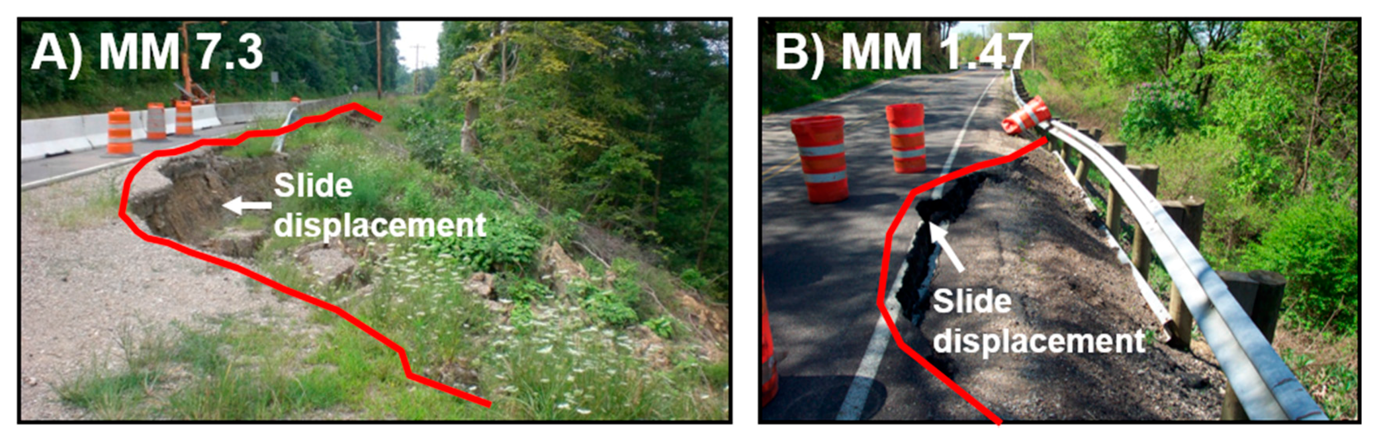
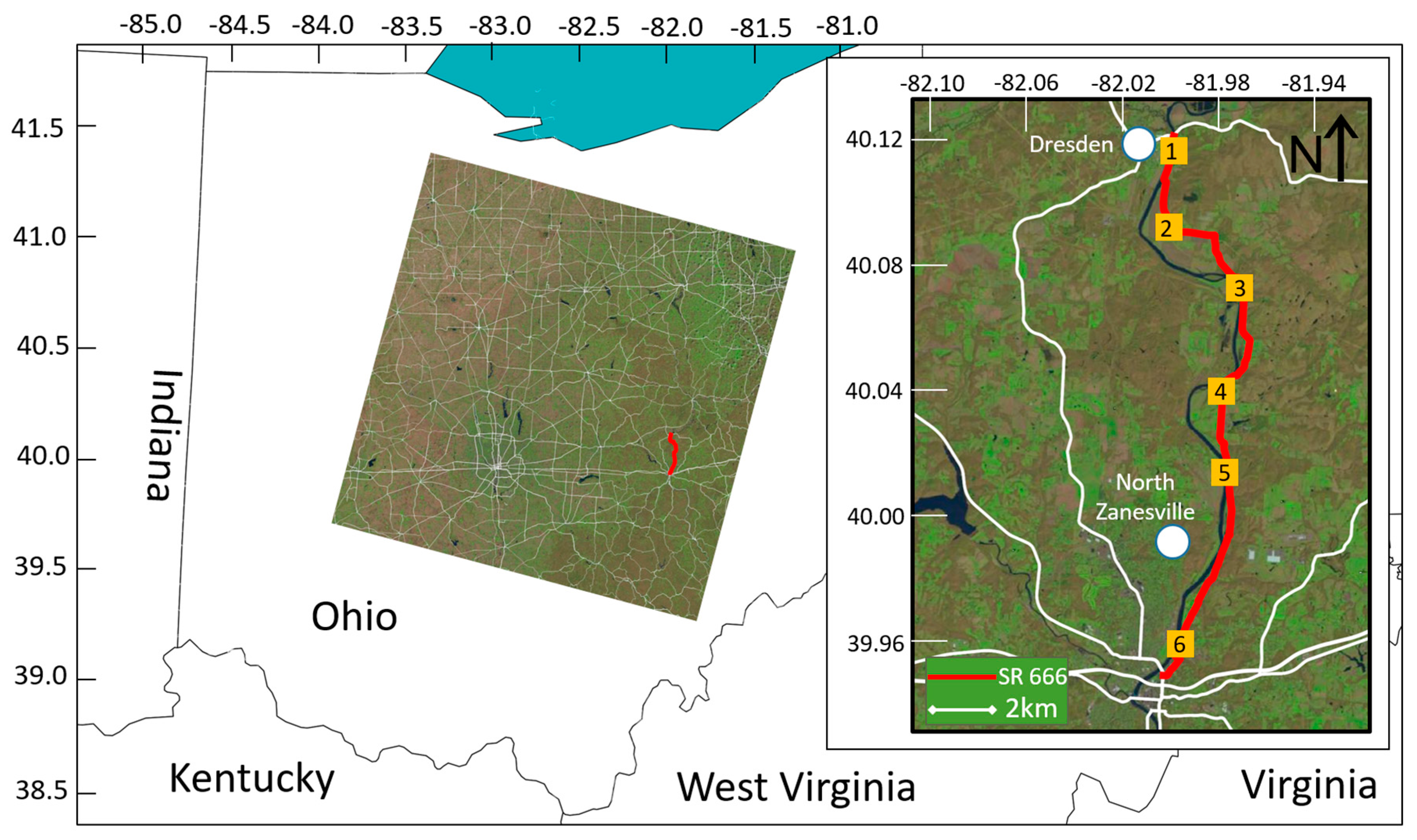
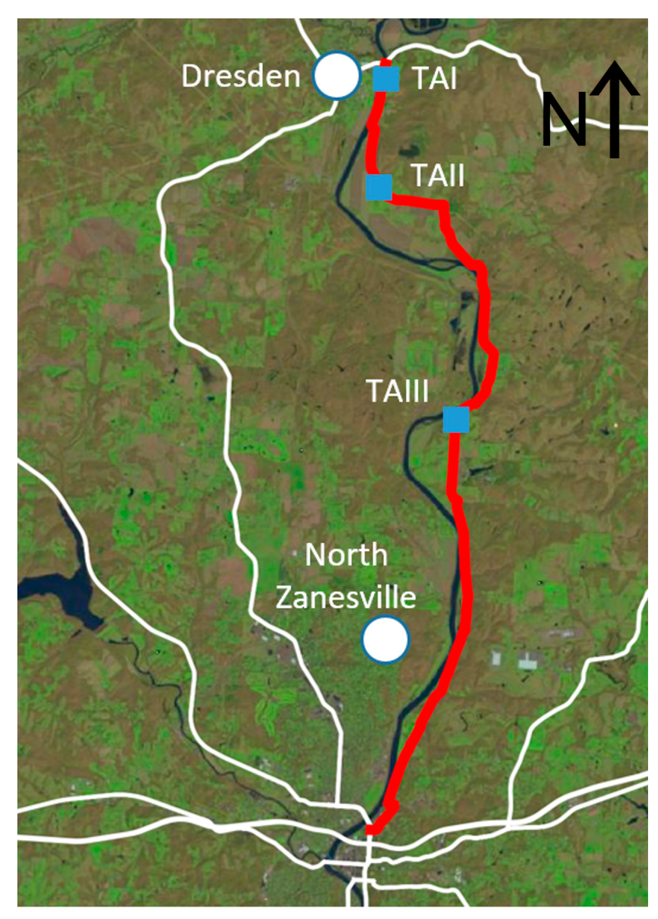
2.1. Study Area
2.2. LiDAR Data
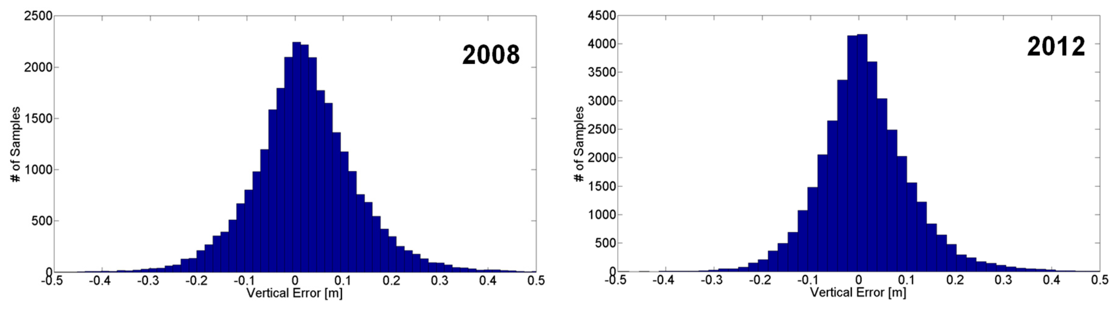
DEM and DoD Uncertainty Evaluation
2.3. Landslide Inventory
3. Methods
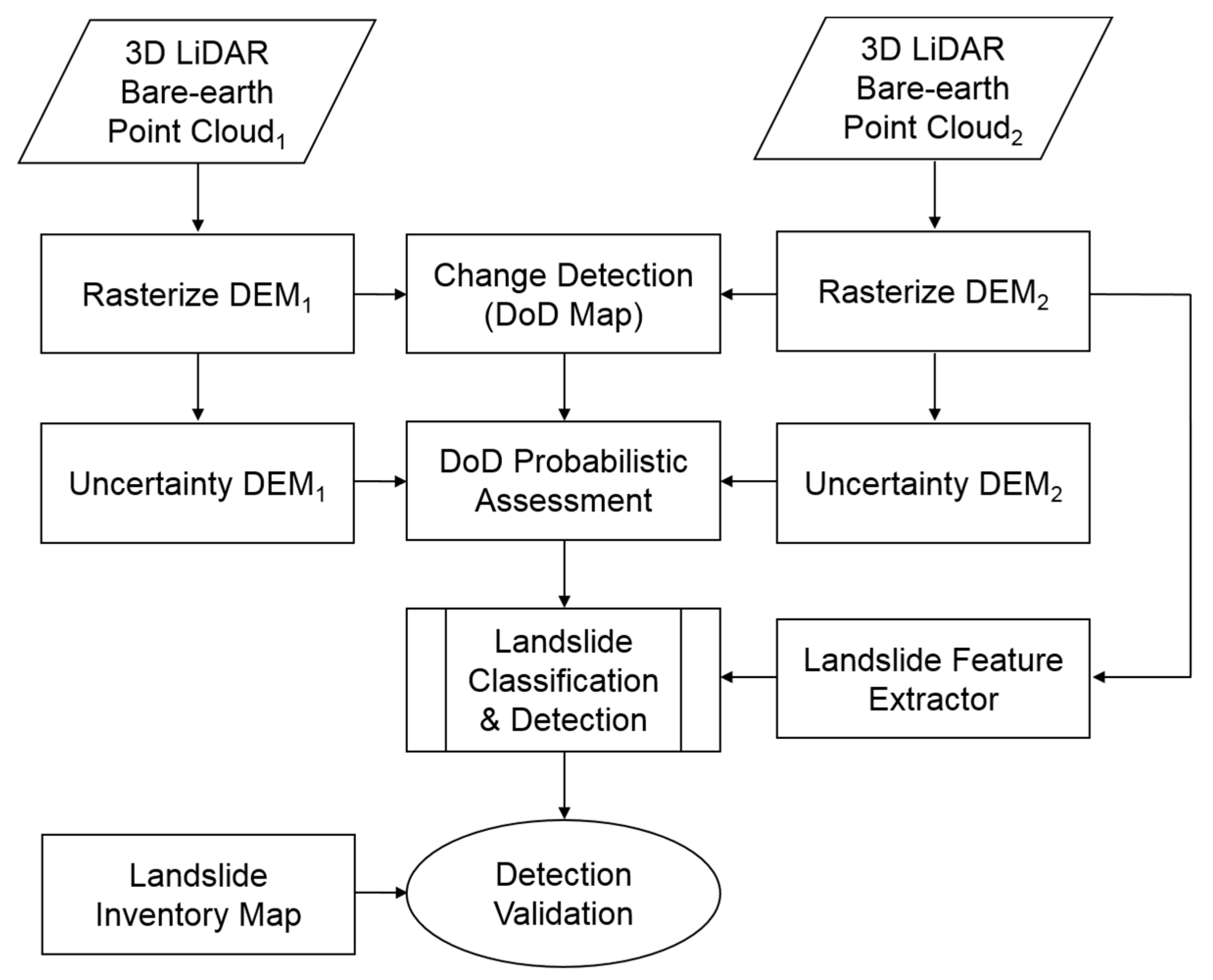
3.1. Algorithm
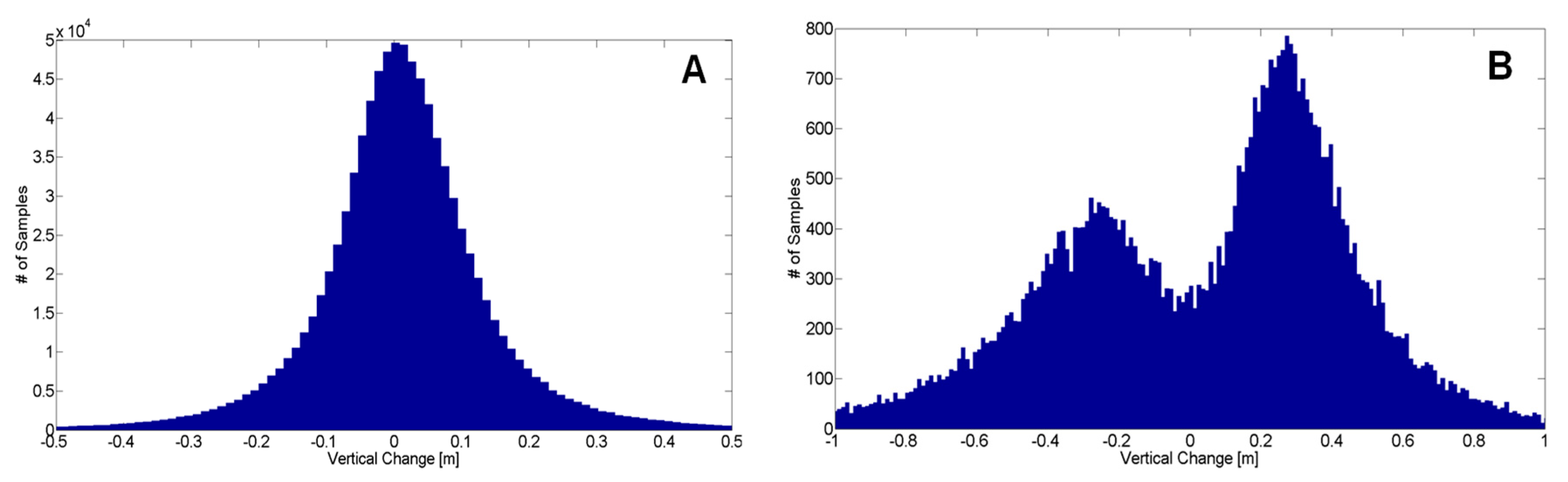
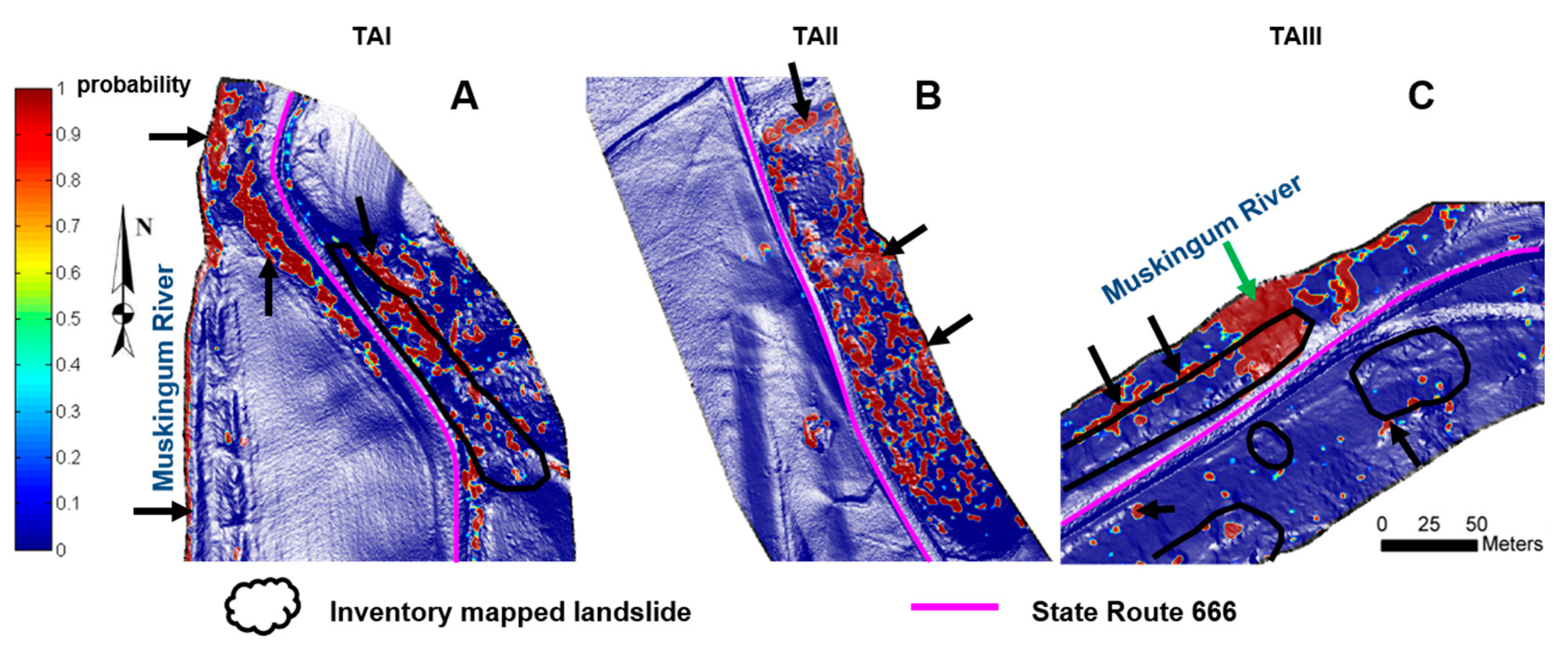
3.2. Probabilistic Change Detection
3.3. Landslide Surface Feature Extraction
Support Vector Machine
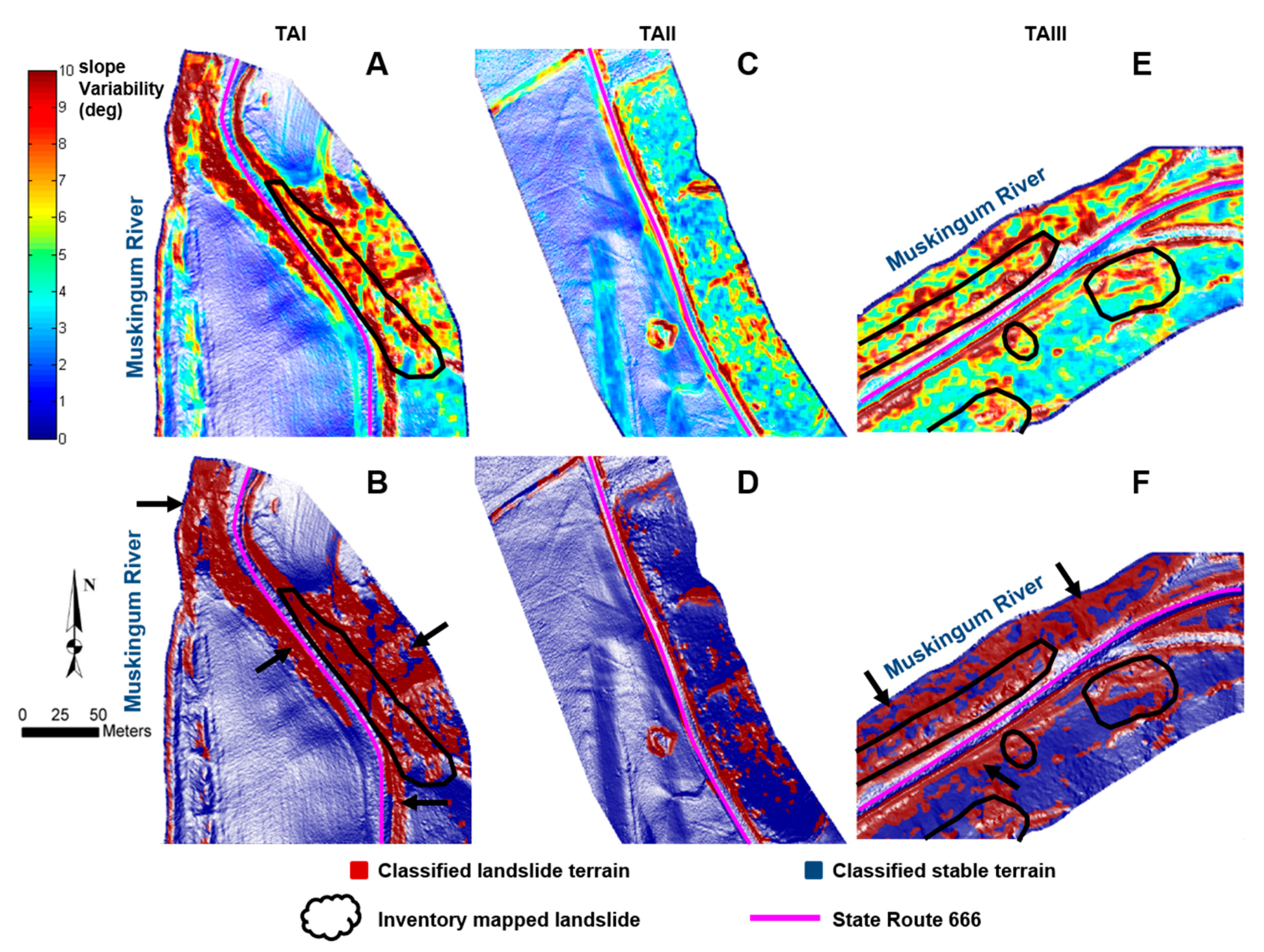
3.4. Landslide Detection
4. Results
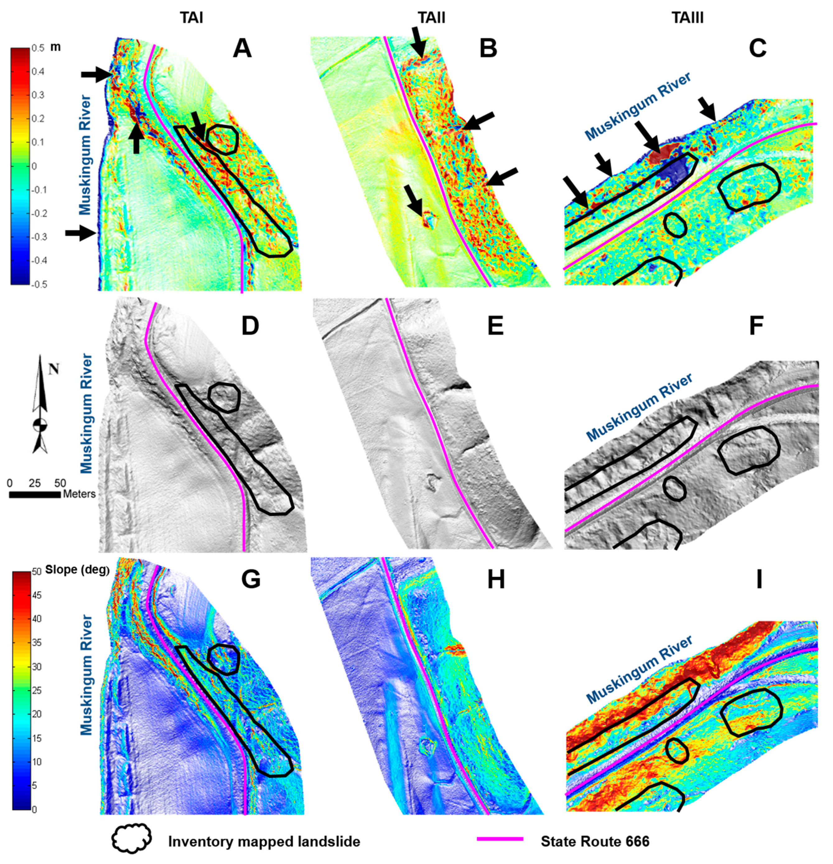
4.1. DEM and DoD Map Evaluation
4.2. Probabilistic Change Detection
4.3. Landslide Surface Feature Extraction
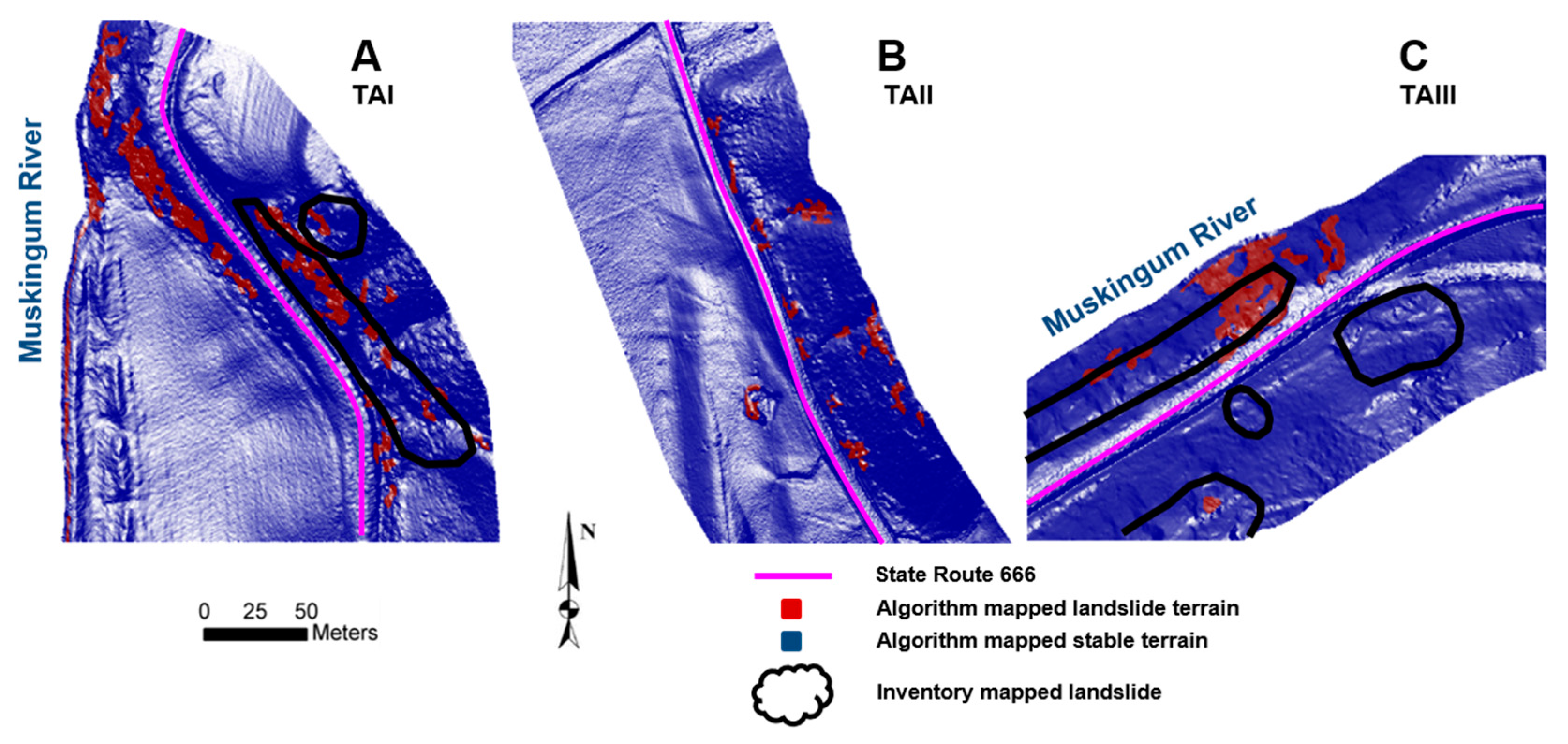
4.4. Landslide Detection
5. Discussion and Conclusions
Acknowledgments
Author Contributions
Conflicts of Interest
References
- Guzzetti, F.; Carrara, A.; Cardinali, M.; Reichenbach, P. Landslide hazard evaluation: A review of current techniques and their application in a multi-scale study, Central Italy. Geomorphology 1999, 31, 181–216. [Google Scholar] [CrossRef]
- Booth, A.M.; Roering, J.J.; Perron, J.T. Automated landslide mapping using spectral analysis and high-resolution topographic data: Puget Sound lowlands, Washington, and Portland Hills, Oregon. Geomorphology 2009, 109, 132–147. [Google Scholar] [CrossRef]
- Martha, T.R.; Kerle, N.; van Westen, C.J.; Jetten, V.; Kumar, K.V. Segment optimization and data-driven thresholding for knowledge-based landslide detection by object-based image analysis. IEEE Trans. Geosci. Remote Sens. 2011, 49, 4928–4943. [Google Scholar] [CrossRef]
- Ballabio, C.; Sterlacchini, S. Support vector machines for landslide susceptibility mapping: The Staffora River Basin case study, Italy. Math. Geosci. 2012, 44, 47–70. [Google Scholar] [CrossRef]
- Tien Bui, D.; Pradhan, B.; Lofman, O.; Revhaug, I. Landslide susceptibility assessment in Vietnam using Support vector machines, Decision tree and Naïve Bayes models. Math. Probl. Eng. 2012, 2012, 974638. [Google Scholar] [CrossRef]
- McKean, J.; Roering, J. Objective landslide detection and surface morphology mapping using high-resolution airborne laser altimetry. Geomorphology 2004, 57, 331–351. [Google Scholar] [CrossRef]
- Galli, M.; Ardizzone, F.; Cardinali, M.; Guzzetti, F.; Reichenbach, P. Comparing landslide inventory maps. Geomorphology 2008, 94, 268–289. [Google Scholar] [CrossRef]
- Wang, L.-J.; Sawada, K.; Moriguchi, S. Landslide-susceptibility analysis using light detection and ranging-derived digital elevation models and logistic regression models: A case study in Mizunami City, Japan. J. Appl. Remote Sens. 2013, 7, 073561. [Google Scholar] [CrossRef]
- Lane, S.N.; Richards, K.S.; Chandler, J.H. Developments in monitoring and modelling small-scale river bed topography. Earth Surface Processes Landf. 1994, 19, 349–368. [Google Scholar] [CrossRef]
- Wheaton, J.M.; Brasington, J.; Darby, S.E.; Merz, J.; Pasternack, G.B.; Sear, D.; Vericat, D. Linking geomorphic changes to salmonid habitat at a scale relevant to fish. River Res. Appl. 2010, 26, 469–486. [Google Scholar] [CrossRef]
- Wheaton, J.M.; Brasington, J.; Darby, S.E.; Sear, D.A. Accounting for uncertainty in DEMs from repeat topographic surveys: Improved sediment budgets. Earth Surf. Processes Landf. 2010, 35, 136–156. [Google Scholar] [CrossRef]
- DeLong, S.B.; Prentice, C.S.; Hilley, G.E.; Ebert, Y. Multitemporal ALSM change detection, sediment delivery, and process mapping at an active earthflow. Earth Surf. Processes Landf. 2012, 37, 262–272. [Google Scholar] [CrossRef]
- Kelsey, H.M. Earthflows in Franciscan mélange, Van Duzen River basin, California. Geology 1978, 6, 361–364. [Google Scholar] [CrossRef]
- Baum, R.L.; Messerich, J.; Fleming, R.W. Surface deformation as a guide to kinematics and three-dimensional shape of slow-moving, clay-rich landslides, Honolulu, Hawaii. Environ. Eng. Geosci. 1998, 4, 283–306. [Google Scholar] [CrossRef]
- Malet, J.-P.; Maquaire, O.; Calais, E. The use of Global Positioning System techniques for the continuous monitoring of landslides: Application to the Super-Sauze earthflow (Alpes-de-Haute-Provence, France). Geomorphology 2002, 43, 33–54. [Google Scholar] [CrossRef]
- Chadwick, J.; Dorsch, S.; Glenn, N.; Thackray, G.; Shilling, K. Application of multi-temporal high-resolution imagery and GPS in a study of the motion of a canyon rim landslide. ISPRS J. Photogramm. Remote Sens. 2005, 59, 212–221. [Google Scholar] [CrossRef]
- Glenn, N.F.; Streutker, D.R.; Chadwick, D.J.; Thackray, G.D.; Dorsch, S.J. Analysis of LiDAR-derived topographic information for characterizing and differentiating landslide morphology and activity. Geomorphology 2006, 73, 131–148. [Google Scholar] [CrossRef]
- Mackey, B.H.; Roering, J.J.; McKean, J.A. Long-term kinematics and sediment flux of an active earthflow, Eel River, California. Geology 2009, 37, 803–806. [Google Scholar] [CrossRef]
- Coe, J.A.; McKenna, J.P.; Godt, J.W.; Baum, R.L. Basal-topographic control of stationary ponds on a continuously moving landslide. Earth Surf. Processes Landf. 2009, 34, 264–279. [Google Scholar] [CrossRef]
- Mackey, B.H.; Roering, J.J. Sediment yield, spatial characteristics, and the long-term evolution of active earthflows determined from airborne LiDAR and historical aerial photographs, Eel River, California. Geol. Soc. Am. Bull. 2011, 123, 1560–1576. [Google Scholar] [CrossRef]
- Cheng, K.S.; Wei, C.; Chang, S.C. Locating landslides using multi-temporal satellite images. Adv. Space Res. 2004, 33, 296–301. [Google Scholar] [CrossRef]
- Lu, P.; Stumpf, A.; Kerle, N.; Casagli, N. Object-oriented change detection for landslide rapid mapping. IEEE Geosci. Remote Sens. Lett. 2011, 8, 701–705. [Google Scholar] [CrossRef]
- Daehne, A.; Corsini, A. Kinematics of active earthflows revealed by digital image correlation and DEM subtraction techniques applied to multi-temporal LiDAR data. Earth Surf. Processes Landf. 2013, 38, 640–654. [Google Scholar] [CrossRef]
- Ventura, G.; Vilardo, G.; Terranova, C.; Sessa, E.B. Tracking and evolution of complex active landslides by multi-temporal airborne LiDAR data: The Montaguto landslide (Southern Italy). Remote Sens. Environ. 2011, 115, 3237–3248. [Google Scholar] [CrossRef]
- Tseng, C.M.; Lin, C.W.; Stark, C.P.; Liu, J.K.; Fei, L.Y.; Hsieh, Y.C. Application of a multi-temporal. LiDAR-derived, digital terrain model in a landslide-volume estimation. Earth Surf. Processes Landf. 2013, 38, 1587–1601. [Google Scholar] [CrossRef]
- Caris, J.P.T.; van Asch, T.W. Geophysical, geotechnical and hydrological investigations of a small landslide in the French Alps. Eng. Geol. 1991, 31, 249–276. [Google Scholar] [CrossRef]
- Garel, E.; Marc, V.; Ruy, S.; Cognard-Plancq, A.L.; Klotz, S.; Emblanch, C.; Simler, R. Large scale rainfall simulation to investigate infiltration processes in a small landslide under dry initial conditions: The Draix hillslope experiment. Hydrol. Process. 2012, 26, 2171–2186. [Google Scholar] [CrossRef]
- James, L.A.; Hodgson, M.E.; Ghoshal, S.; Latiolais, M.M. Geomorphic change detection using historic maps and DEM differencing: The temporal dimension of geospatial analysis. Geomorphology 2012, 137, 181–198. [Google Scholar] [CrossRef]
- Wehr, A.; Lohr, U. Airborne laser scanning—An introduction and overview. ISPRS J. Photogramm. Remote Sens. 1999, 54, 68–82. [Google Scholar] [CrossRef]
- Shan, J.; Toth, C.K. (Eds.) Topographic Laser Ranging and Scanning: Principles and Processing; CRC Press: Boca Raton, FL, USA, 2008. [Google Scholar]
- Ohio Department of Transportation Office of Geotechnical Engineering. Report of Findings, Geohazard Inventory and Evaluation, MUS-666-0.00. Available online: www.dot.state.oh.us/Divisions/Planning/SPR/Research/reportsandplans/Reports/2015/Geotechnical/134609_ES.pdf (accessed on 20 November 2017).
- Isenburg, M. LAStools—Efficient Tools for LiDAR Processing. Version 111216. Available online: http://lastools.org (accessed on 20 November 2017).
- Mora, O.E.; Lenzano, M.G.; Toth, C.K.; Grejner-Brzezinska, D.A. Analyzing the Effects of Spatial Resolution for Small Landslide Susceptibility and Hazard Mapping. Int. Arch. Photogramm. Remote Sens. Spat. Inf. Sci. 2014, XL-1, 293–300. [Google Scholar] [CrossRef]
- Brasington, J.; Langham, J.; Rumsby, B. Methodological sensitivity of morphometric estimates of coarse fluvial sediment transport. Geomorphology 2003, 53, 299–316. [Google Scholar] [CrossRef]
- Wilcoxon, F. Individual comparisons by ranking methods. Biometrics 1945, 1, 80–83. [Google Scholar] [CrossRef]
- Hollander, M.; Wolfe, D.A.; Chicken, E. Nonparametric Statistical Methods; John Wiley & Sons: New York, NY, USA, 2013; Volume 751. [Google Scholar]
- Mora, O.E.; Liu, J.K.; Lenzano, M.G.; Toth, C.K.; Grejner-Brzezinska, D.A. Small Landslide Susceptibility and Hazard Assessment Based on Airborne Lidar Data. Photogramm. Eng. Remote Sens. 2015, 81, 239–247. [Google Scholar] [CrossRef]
- Vapnik, V. The Nature of Statistical Learning; Springer: New York, NY, USA, 2000. [Google Scholar]
- Samui, P. Slope stability analysis: A support vector machine approach. Environ. Geol. 2008, 56, 255–267. [Google Scholar] [CrossRef]
- Yao, X.; Tham, L.G.; Dai, F.C. Landslide susceptibility mapping based on support vector machine: A case study on natural slopes of Hong Kong, China. Geomorphology 2008, 101, 572–582. [Google Scholar] [CrossRef]
- Marjanović, M.; Kovačević, M.; Bajat, B.; Voženílek, V. Landslide susceptibility assessment using SVM machine learning algorithm. Eng. Geol. 2011, 123, 225–234. [Google Scholar] [CrossRef]
- Micheletti, N.; Foresti, L.; Kanevski, M.; Pedrazzini, A.; Jaboyedoff, M. Landslide Susceptibility Mapping Using Adaptive Support Vector Machines and Feature Selection. Master’s Thesis, University of Lausanne, Lausanne, Switzerland, 2011; 99p. [Google Scholar]
- Katzil, Y.; Doytsher, Y. A logarithmic and sub-pixel approach to shaded relief representation. Comput. Geosci. 2003, 29, 1137–1142. [Google Scholar] [CrossRef]
- Nichol, J.; Wong, M.S. Satellite remote sensing for detailed landslide inventories using change detection and image fusion. Int. J. Remote Sens. 2005, 26, 1913–1926. [Google Scholar] [CrossRef]


| Segment # | No. Pts | Mean (m) | STD (m) | Min (m) | Max (m) | RMSE (m) | ||||||
|---|---|---|---|---|---|---|---|---|---|---|---|---|
| 2008 | 2012 | 2008 | 2012 | 2008 | 2012 | 2008 | 2012 | 2008 | 2012 | 2008 | 2012 | |
| 1 | 4241 | 5448 | 0.05 | 0.02 | 0.12 | 0.12 | 0.00 | 0.00 | 0.82 | 0.76 | 0.12 | 0.12 |
| 2 | 3181 | 3710 | 0.01 | 0.01 | 0.14 | 0.07 | 0.00 | 0.00 | 0.84 | 0.55 | 0.14 | 0.08 |
| 3 | 7589 | 10,057 | 0.06 | 0.02 | 0.09 | 0.09 | 0.00 | 0.00 | 0.58 | 0.55 | 0.11 | 0.09 |
| 4 | 4610 | 6597 | −0.03 | 0.01 | 0.08 | 0.08 | 0.00 | 0.00 | 0.32 | 0.34 | 0.08 | 0.08 |
| 5 | 4564 | 5460 | −0.02 | 0.02 | 0.13 | 0.13 | 0.00 | 0.00 | 0.72 | 0.71 | 0.13 | 0.13 |
| 6 | 4866 | 7125 | 0.04 | 0.01 | 0.08 | 0.09 | 0.00 | 0.00 | 0.67 | 1.29 | 0.09 | 0.09 |
| Total | 29,051 | 38,397 | 0.02 | 0.01 | 0.11 | 0.10 | 0.00 | 0.00 | 0.84 | 1.29 | 0.11 | 0.10 |
| Testing Areas | Mean (m) | Median (m) | STD (m) |
|---|---|---|---|
| TAI | 0.01 | 0.01 | 0.18 |
| TAII | 0.07 | 0.05 | 0.12 |
| TAIII | −0.03 | 0.00 | 0.29 |
| Changes Detected (Units: m) | Mean | Median | STD |
|---|---|---|---|
| Inventory Mapped Slides (A) | 0.01 | 0.02 | 0.17 |
| Algorithm Mapped w/in Inventory Slides (B) | 0.02 | 0.18 | 0.48 |
© 2018 by the authors. Licensee MDPI, Basel, Switzerland. This article is an open access article distributed under the terms and conditions of the Creative Commons Attribution (CC BY) license (http://creativecommons.org/licenses/by/4.0/).
Share and Cite
Mora, O.E.; Lenzano, M.G.; Toth, C.K.; Grejner-Brzezinska, D.A.; Fayne, J.V. Landslide Change Detection Based on Multi-Temporal Airborne LiDAR-Derived DEMs. Geosciences 2018, 8, 23. https://doi.org/10.3390/geosciences8010023
Mora OE, Lenzano MG, Toth CK, Grejner-Brzezinska DA, Fayne JV. Landslide Change Detection Based on Multi-Temporal Airborne LiDAR-Derived DEMs. Geosciences. 2018; 8(1):23. https://doi.org/10.3390/geosciences8010023
Chicago/Turabian StyleMora, Omar E., M. Gabriela Lenzano, Charles K. Toth, Dorota A. Grejner-Brzezinska, and Jessica V. Fayne. 2018. "Landslide Change Detection Based on Multi-Temporal Airborne LiDAR-Derived DEMs" Geosciences 8, no. 1: 23. https://doi.org/10.3390/geosciences8010023
APA StyleMora, O. E., Lenzano, M. G., Toth, C. K., Grejner-Brzezinska, D. A., & Fayne, J. V. (2018). Landslide Change Detection Based on Multi-Temporal Airborne LiDAR-Derived DEMs. Geosciences, 8(1), 23. https://doi.org/10.3390/geosciences8010023