Kinematic Reconstruction of a Deep-Seated Gravitational Slope Deformation by Geomorphic Analyses

Abstract

On 4 November 2010, a deep-seated gravitational slope deformation (North Italy) reactivated with sudden ground movement. A 450,000 m² mountainous area moved some metres downslope, but the undeniable signs were only connected to the triggering of a debris flow from the bulging area’s detrital cover and the presence of a continuous perimeter fracture near the crown area. Based on two detailed LiDAR surveys (2 m × 2 m) performed just a few days before and after the event, a quantitative topographic analysis was performed in a GIS environment, integrating morphometric terrain parameters (slope, aspect, surface roughness, hill shade, and curvature). The DEMs analysis highlighted some morphological changes related to deeper as well as shallow movements. Both global and sectorial displacements were widely verified and discussed, finally inferring that the geometry, persistence, and layout of all movements properly justify each current morphostructure, which has the shape of a typical Sackung-type structure with impulsive kinematics. Moreover, a targeted field survey allowed specific clues to be found that confirmed the global deduced dynamics of the slope deformation. Finally, thanks to a ground-based interferometric radar system (GB-InSAR) that was installed a few days after the reactivation, the residual deep-seated gravitational slope deformation (DSGSD) movements were also monitored. In the landslide lower bulging area, a localized material progression of small entities was observed for some months after the parossistic event, indicating a slow dissipation of forces in sectors more distant from the crown area.

1. Introduction

Among natural hazards, slope instability processes in mountainous areas are characterized by complex interactions among different lithological, geomorphological, and structural features (topographical location, size, and connection with the drainage network) and processes (triggering factors, styles of activity, and displacements) [1,2,3,4]. Some of the largest non-catastrophic slow rock-slope deformations affecting entire high-relief valley walls are deep-seated gravitational slope deformations (DSGSDs) [2,4,5,6], and according to Dramis et al. [1] and Agliardi et al. [3], most of these are Sackung type [2,7,8,9]. Although DSGSDs have been recognized since the 1940s [10], the phenomenon was poorly understood until the 1990s, when the multidisciplinary research approach and new technologies began to be used [3,9]. According to Bovis [9], a precise definition of DSGSDs is problematic. Even though a general agreement has been found around the classification based on movement type and involved materials proposed by Cruden and Varnes [5], there are many definitions that depend on study approach and postulated evolutionary mechanisms. There is a wide literature on DSGSD definition, classification, and the most frequently quoted predisposing, controlling or causal factors [2,3,4,6,9,10,11].

In general terms, DSGSDs

(i)

occur on high relief-energy hillslopes involving entire valley flanks (the extension could range from the ridge crest to the valley floor) [2,4,6,10];

(ii)

have sizes comparable to whole slopes (from few cubic metres to thousands or tens of millions of cubic metres) [3,5,12,13];

(iii)

can be found in different rock types and are mostly characterized by poorly defined and/or irregular lateral boundaries [2,6,13]. Subsurface geometry is often unknown, but the absence of a macroscopically well-denoted slip surface cannot be assumed to be a DSGSD diagnostic feature [6]. In fact, many confined landslides [5,8] do not show a clear or complete sliding surface until final collapse, and, on the other hand, many DSGSDs are characterized by basal sliding surfaces [10,14];

(iv)

display gravitational morphostructures (e.g., large scarps and counterscarps or up-hill facing scarps, open or infilled trenches, downthrown blocks, ridge top depressions or toe bulging, open tension cracks, grabens, double or multiple ridges) [4,6,10,13,14] and geomorphological evidence of slope deformation and displacements along individual structures and inherited structural features [4]. Nevertheless, it is not yet clear if tectonic features play an active or passive role in DSGSD movements (i.e., DSGSDs occur in zones of high stress or simply in weak rock) [6] and, therefore, whether the sliding surface is occasionally partially coincident to a pre-existing tectonic surface or whether it must be postulated to justify the DSGSD kinematics [10];

(v)

have low displacement rates (mm/year) compared to those of the slopes themselves that are often undetectable because of weathering or erosion [2,6,10,13] and/or because the rates are close to the detection precisions of monitoring instruments [5,9]; and

(vi)

trigger sudden and rapid secondary minor landslides (rotational and planar slides, falls, topples and debris flows) from the most superficial part [10,15,16] or can evolve in huge landslides of different types after very long evolutionary phases [1], so that DSGSDs can be considered as preparation stages for huge gravitational collapses that, in any event, do not always complete their evolution [1,2].

The worldwide distribution map of the most significant DSGSDs studied since the 1990s [14] shows that they are not rare in mountain belts. DSGSDs are common in Europe, and there are four main DSGSD published databases [14]: Scottish Highlands (89 landslides), Eastern Pyrennes (30 landslides), European Alps (1033 landslides), and Western Carpathians (more than 100 landslides). The updated European Alps DSGSD inventory is presented and discussed in [4], together with some general criteria for the generation of a homogeneous and reliable DSGSD inventory. Some studies suggest that more than 5% of alpine slopes are affected by DSGSDs [4,11].

Until recently, DSGSD were considered inactive and non-hazardous phenomena under present climatic conditions because of their slow evolution [2]. Nevertheless, under certain conditions, movements can last for long periods, resulting in large cumulative displacements. However, after periods of inactivity, external agents (exceptionally heavy rainfall periods, groundwater recharge, snow melts, temperature oscillations, and earthquakes) can reactivate them, and they can show episodic accelerations that can sometimes reach alarming levels but then subside to non-critical levels [1,17], evolve into faster mass movements or favour collateral landslide processes [2,14]. Consequently, DSGSDs can also be considered hazardous phenomena because they can cause deformations in structures and infrastructures, i.e., buildings, roads, railway tracks, tunnels, underground caverns, dams, hydroelectric power stations and penstocks [5,6,9,17,18].

DSGSDs can be triggered by different and potentially coexisting mechanisms, as discussed in [3,14,17,19], so studies can focus on both initial failure and successive reactivations or each separately [20]. Moreover, DSGSDs evolve at long-term (≥10² years) and short-term (<10² years) times scales according to Pánek and Klimeš [14], and a multidisciplinary approach is necessary to understand the overall geometry and kinematics of DSGSDs and assess correct mitigation procedures [3,14,18]. In the short term, conventional DSGSD displacement monitoring methods are usually adopted, which provide information on a limited number of points (geotechnical in situ instrumentation such as inclinometers and extensometers, topographic or GPS surveys) [14,21,22], but usually the obtained data are insufficient to assess whole landslide kinematics and behaviour [21] or estimate expected collapse time [20]. Therefore, advanced remote sensing methodologies that are chiefly based on satellite, aerial and terrestrial technologies have gained widespread recognition as efficient tools for characterizing and monitoring landslide-affected areas in terms of resolution, accuracy, data visualization, management, and reproducibility [14,23,24,25,26]. Among all the terrestrial and aerial remote sensing technologies applied in landslide analysis, those that are more effective for DSGSD studies are ground-based interferometric radar (GB-InSAR, [21,24,25,27]), and light detection and ranging (LiDAR, [19,28]). However, compared with their use in other landslides, applications of advanced remote sensing techniques and/or geophysical investigations [29,30,31] remain rarely applied to DSGSDs [14].

This paper addresses the Rotolon DSGSD (north-eastern Italy), and the main goal is to understand its kinematic behaviour after the October-November 2010 rainfalls, which apparently does not show direct reactivation clues but only more hazardous localized and secondary phenomena such as debris flows and rock falls. Therefore, all previous studies of the Rotolon landslide were aimed at characterizing the landslide morphological features, assessing the landslide residual displacements, and supporting local authorities in emergency management. In fact, a GB-InSAR monitoring system [25,27] and an automatic monitoring network and early-warning system [22] were installed, and accurate geomorphological field surveys [15] and infrared thermographic (IRT) analysis [18,32] were carried out. Moreover, a 3D landslide runout numerical model was used to identify the source and impact areas of potential debris flow events, flow velocity and deposit distribution within the Rotolon creek valley [16,33].

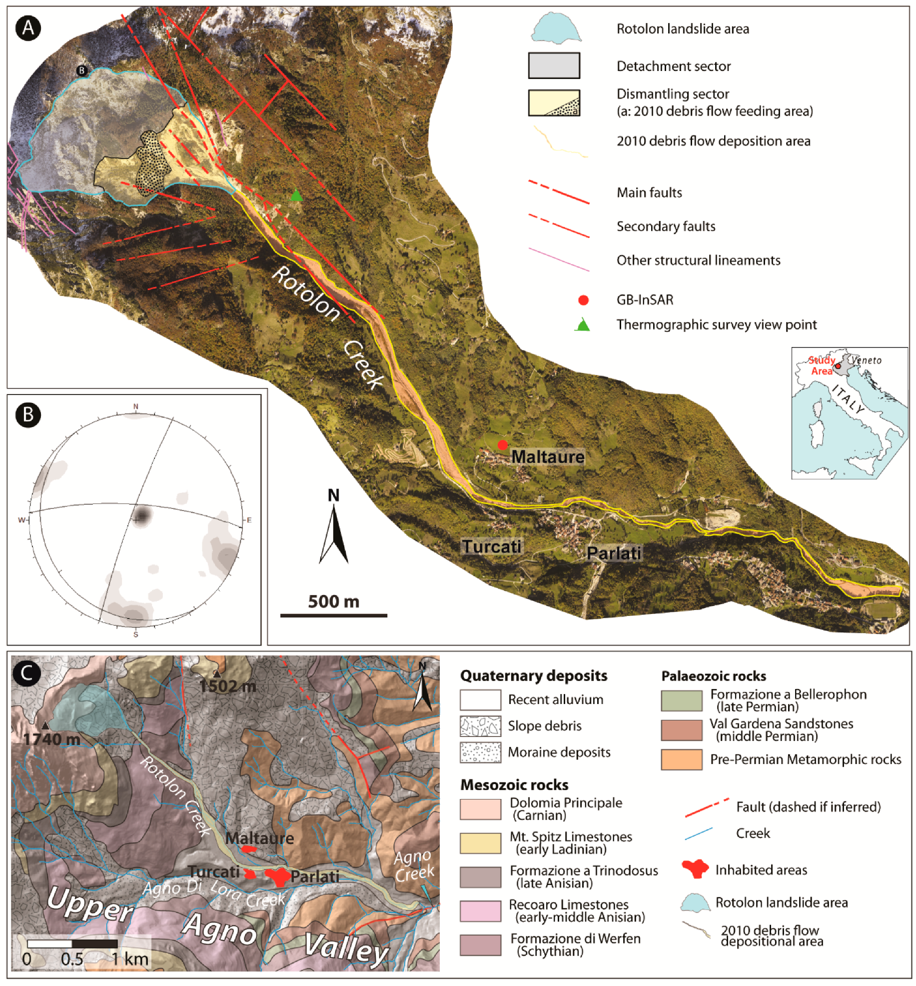
2. Study Area

2.1. Geology and Geomorphology

The Rotolon DSGSD is located in the Little Dolomites chain (Vicentine Prealps, Veneto, Italy, Figure 1), in the topmost slopes of the Rotolon River Basin (the extension of which is approximately 5 km²), which is part of the Upper Agno valley (Figure 1). The slope instability processes in this area, which is characterized by both slow phenomena (such as localized debris slides and the studied DSGSD) and rapid slope failures (such as large debris flows, rock avalanches, rockfalls and topples), have threatened the valley for centuries, as documented in a recent bibliography [34,35,36] and historical documents available since 1573 [37]. Moreover, the local toponym suggests the dangerousness of such slopes. The Rotolon name, in fact, originates from the language of an ancient local Celtic population (Cimbri) through the composition of rot (red) with lön (landslide) [37].

The Rotolon DSGSD, which is already included in the 2008 DSGSD inventory [4], covers an area of approximately 450,000 m² and has a drop height of 600 m (from approximately 1700 m to 1100 m above see level). It overtops a narrow poorly populated s-shaped valley that is often threatened by rapid channelled landslide occurrences (Figure 1). Such deformational activity develops in the uppermost portion of a sub-horizontally bedded, intensively fractured, mainly dolomitic limestone stratigraphic succession belonging to the South Alpine Domain (middle Triassic to lower Jurassic in age) [15,25]. The geological formations, from bottom to top, are the Mt. Spitz Limestone (massive, locally layered limestones), Raibl Formation (a sequence of conglomerates, sandstones, marls and dolomitic evaporates that show a discontinuous level of riolitic-dacitic porphyrites at the bottom), and Dolomia Principale (dolostones and dolomitic limestones). Two main low-displacement fault systems (NE-SW and NNW-SSE oriented) and a third one (E-W oriented) intersect the area (Figure 1A) [35]. Structural discontinuities with the same geometric pattern were also identified by photo interpretation on the west rocky massif bordering the studied area (Figure 1A) and along the ridge next to the main crown (Figure 1B) by collecting the orientations of discontinuities [38,39]. Such a spatial distribution and related structural constraint contributed to develop the current amphitheatre shape of the DSGSD and influenced the deformational character of the entire slope.

On the basis of the geomorphological analysis, the whole DSGSD can be divided into two main zones (Figure 1A): (i) an upper detachment sector (mean slope of approximately 30°), which develops large extensional forms that reduce the average slope inclinations, and (ii) a lower dismantling or bulging sector (mean angle of approximately 34°) that includes high-angle slopes with compressive arched forms [15].

Many linear landforms that are related to the relaxing consequences of gravitational action such as tensional fractures along scarps (Figure 2B (ii)), trenches and crests (Figure 2C) that are largely associated with colluvial, rockfall and rock avalanche materials with very coarse and heterometric clasts and scattered boulders (Figure 2B (i)) are widely recognized and mapped in the detachment sector [15,25]. No evidence of glacial phenomena has been identified in those materials, even though active earth-shaping agents such as karst phenomena, which are able to rapidly modify the territory with their own morphological forms, are absent. Even glacial deposits are absent here, and according to Altieri [35], they are only distributed in a narrow south-east area of the basin outside the DSGSD. Toe bulging structures such as tilted mega blocks and subvertical open fractures (Figure 2D,E) have instead been documented in the dismantling sector through some outcrops. In fact, a large and thick loose detritus mantle originated by short-term surface processes is predominant and widespread in the bulging sector and masks the continuity of the local deformations, especially in the lowermost portions (Figure 2F,G) [16,25]. In this area, however, no well-denoted slip surface associable with other types of possible mass movements (e.g., rockslides) has been found or directly and indirectly outlined by topographic examinations. Therefore, the evidence of extensional and compressive processes in the uppermost and lowermost parts of the landslide, respectively, joined with the rough morphology suggest that the Rotolon DSGSD can be classified as Sackung [7,15]. Moreover, regarding its general structure, this slope deformation can be classified at the limit between large landslides and DSGSDs on the basis of the area-frequency statistics proposed by Agliardi et al. [3].

2.2. The 2010 DSGSD Reactivation

Between 31 October 2010, and 2 November 2010, the entire Veneto region was hit by heavy and persistent rainfall after a rather rainy period that led to diffuse landslide events [22,25]. These rainfalls triggered widespread flooding and abundant slope failures and caused 3 fatalities, the evacuation of approximately 3500 people, extensive damage to structures and heavy economic losses in agricultural, livestock, and industrial activities. On 4 November 2010, a dormant Deep-Seated Gravitational Slope Deformation reactivated with sudden ground movement on the south-east facing slope of the Rotolon River Basin. A 450,000 m² mountainous area moved downslope, but the undeniable signs were only connected to the triggering of a debris flow from the detrital cover of the bulging area and the presence of a continuous perimeter fracture near the crown area associable with the geomorphic expression of the surface sliding (Figure 3). The detachment of this subordinate mass movement, which was approximately 320,000 m³ in volume, channelized in the downstream Rotolon Creek, damaging various hydraulic works and structures related to the settlements located along the creek beds [16,32]. This critical situation has drawn new attention to the geo-hydrological hazards of the valley, and new efforts were actuated by the Civil Protection to address this problem in detail. In particular, the first contingent interventions were focused on the debris flow source area by means of instrumental measurements [18,22,25,27,32] and field surveys [15], and they were later extended to the whole DSGSD area.

3. Materials and Methods

3.1. LiDAR Measurement

To provide information on the nature, extent and activation frequency of ancient gravitational slope movements, standard detection and mapping procedures employ a combination of field-based studies and advanced techniques such as remote sensing data analysis and geophysical investigations [23,29,40,41,42]. The LiDAR technique is currently commonly used in landslide inventory mapping and more generally in geomorphology and natural hazards fields to understand landslide evolution and geomorphological processes [19,28]. Airborne and ground-based sensors send out pulses and record the returning signals that are back-scattered by the ground surface and other objects. A complete review of these techniques is presented in [28]. From the large amounts of LiDAR terrain 3D information, it is possible to derive high-resolution digital terrain models (DTMs) and compare LiDAR-derived DTMs obtained from successive surveys [36].

Two LiDAR surveys of the Rotolon valley were acquired with the same characteristics by the Soil Defence Department of the Veneto region on 21 October 2010 (denoted pre- in the following), just 13 days before the 2010 debris flow, and on 23 November (denoted post- in the following). An ALTM3100EA laser scanner (Optech, Vaughan, Canada) with a pulse repetition frequency that ranged from 33 kHz to 100 kHz was used to collect data. The instrument was installed on a helicopter, which was flown at a mean speed of 140 km/h. A kinematic GPS [43,44] with dual frequency receivers and oriented by an inertial measurement unit (roll accuracy: 0.02°, pitch accuracy: 0.04°) and one GPS ground station were used to locate the entire LiDAR dataset. The GPS ground station (Parrocchia, 45°46′36.83705″ N, 11°7′22.90136″ E), which was located 6–10 km north-west of the surveyed area, was part of the Trento province GPS Network. The elevations of test area points located throughout the survey area were checked by ground survey data, and the average elevation difference was found to be −0.047 m, with a 0.072 m root mean square (RMS) and a 0.055 standard deviation. The average point densities for both the October and November surveys were approximately 8 pts/m², and the vertical accuracy RMSs were 0.072 m and 0.044 m, respectively. The TerraScan software was used to filter and process the entire dataset and obtain the 2 m × 2 m DEM.

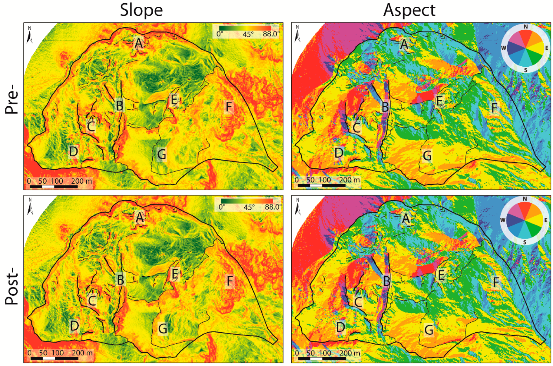
3.2. DEM Analysis

As defined by Evans [45] and Li et al. [46], a landform can be usefully described by five landform parameters: altitude and its first and second derivatives such as gradient, aspect, profile and plan curvature. Moreover, topographic wetness index (TWI) can also be used to characterize landslide roughness [47]. To detect displacement indicators of the Rotolon DSGSD and perform a kinematic analysis (determine the average vertical and horizontal movements and detect zones characterized by different types of activity, recognizing uplift zones) the pre- and post-high-resolution DEM and their (i) slopes, (ii) aspects, (iii) surface roughnesses, (iv) hill shades, (v) curvatures, and (vi) TWI were elaborated and compared in a GIS environment. A combined analysis of slope, aspect, and hill shade, as shown in [15], was also employed to (i) delimit the boundary of the mass movement, (ii) estimate the 2010 debris flow volumes and (iii) identify morphological features such as major and minor scarps, ridges, and cracks.

According to Evans [45] and Li et al. [46], slope is defined at a given point by a plane tangent to the surface and completely identified by gradient (the first vertical derivative, which ranges from 0° to 90°) and aspect (the first horizontal derivative, measured clockwise from 0° to 360°), which are the maximum rate of change of altitude with horizontal displacement and the direction of that maximum in the x-y plane, respectively. Moreover, curvature, the second derivative of the altitude surface, could be defined as the slope change rate, and its two components are profile convexity (the gradient rate of change along a slope line) and plan convexity (the aspect rate of change along a contour). Roughness is the measure of terrain irregularity, and because it is a vague and complex topic, there are many definitions in the literature [45,48,49]. Hillshading is a well-known and useful way of describing the topographic relief of a site using shading to enhance the visualization of objects perpendicular to the azimuth of the illumination [49]. Finally, TWI is defined as the natural logarithm of the ratio between the local upslope area draining through a certain point per unit contour length and the tangent of the slope at that point [50].

The abovementioned parameters (slope, aspect, surface roughness, hill shade, and curvature) presented herein were estimated in ArcGIS 10.4 (Esri, Redlands, CA, USA) using the DEM Surface Tool developed by Jenness [48]. Slope and aspect were calculated using the 4-cell method [51], which is the most accurate method [52], and surface roughness was calculated using the ratio between the surface area and the flat area of square cells [46,53] so that flat areas have values close to 1. The hill shades were obtained using both the same algorithm implemented in the ArcGIS Spatial Analyst tool [48] and the Multidirectional Oblique-Weighted (MDOW) method [48,54], which generated the final hill shade weighting, and according to the cell aspect, the hill shades were generated from 4 directions that were separated by 45° and covered a range of 135°. Finally, the curvature (plan, profile, tangential, and total) was calculated using the Evans approach that uses a 3 × 3 cell moving window, and the curvature was calculated by fitting a curve to the 9 elevation points using a 6-parameter polynomial [45,48]. The TWI maps were obtained in ArcGIS 10.4 starting from the slope (expressed in radians) and the flow accumulation raster according to the equation TWI = ln(flow accumulation/tan(slope_rad)) [50]. High TWI values represent drainage depressions, whereas lower or sometimes negative values represent crests and ridges.

Moreover, maps of residual topographic surface (RTS, [55,56]) were also calculated to highlight the fine scale landforms. These maps were obtained by subtracting from the 2 m × 2 m DEMs a smoothed map created by averaging the values within an n-cells moving window such that each cell of the smoothed DEM has a value that corresponds to the mean of the n² neighbourhood cells values [55].

3.3. GB-InSAR Analysis

The DEM parameter analysis was integrated with incremental and monthly cumulated displacement maps obtained from the GB-InSAR monitoring system described in [25]. GB-InSAR is a computer-controlled microwave antenna that both transmits and receives and moves along a linear rail [57]. SAR images contain information (amplitude and phase) on backscattered echoes of objects observed in investigated scenarios. By evaluating the phase differences, pixel by pixel, between two pairs of complex SAR images, 2D displacement maps along the sensor’s LOS (line of sight; [57]) can be obtained.

The GB-InSAR system, which acquired data every 10 min, was installed in the Maltaure village at an average distance of 3 km from the study area and pointed upwards to the NW (Figure 1). Consequently, the dismantling sector had good spatial coverage, whereas the detachment sectors suffered shadowing effects that were caused by slope roughness, crests, and counter-slope surfaces. Ten measuring points (corresponding to a 5 × 5 pixel area) were selected in correspondence with high stability signal sectors in order to monitor the DSGSD kinematics and characterize the various physiographic features of the slope deformation.

4. Results

The analysis of the DEM parameters allowed some morphological changes to be highlighted that occurred after the October 2010 reactivation and that were associable with deep as well as shallow movements. The difference of DEM (DoD) highlighted negative differences at the boundaries of the 2010 debris flow source area (1 and 2 in Figure 4A,B). These differences were generated by superficial movements, as also confirmed by the field survey (red arrows in Figure 4B). Moreover, the positive anomalies north-east of the 2010 debris flow (3 in Figure 4A,C) could be justified only by taking into account a general and deeper movement of the entire landslide.

The pre- and post-DEM aspect and slope maps are shown in Figure 5, and the roughness and TWI maps are shown in Figure 6. Maps of the differences of these four parameters are also presented in both figures. The maps clearly show that the morphological changes occurred in the entire DSGSD, not just in the area affected by the 4 November debris flow (G in Figure 5 and Figure 6). Six main areas (A–F in Figure 5, Figure 6 and Figure 7) were identified based on the distribution of the surface irregularities. 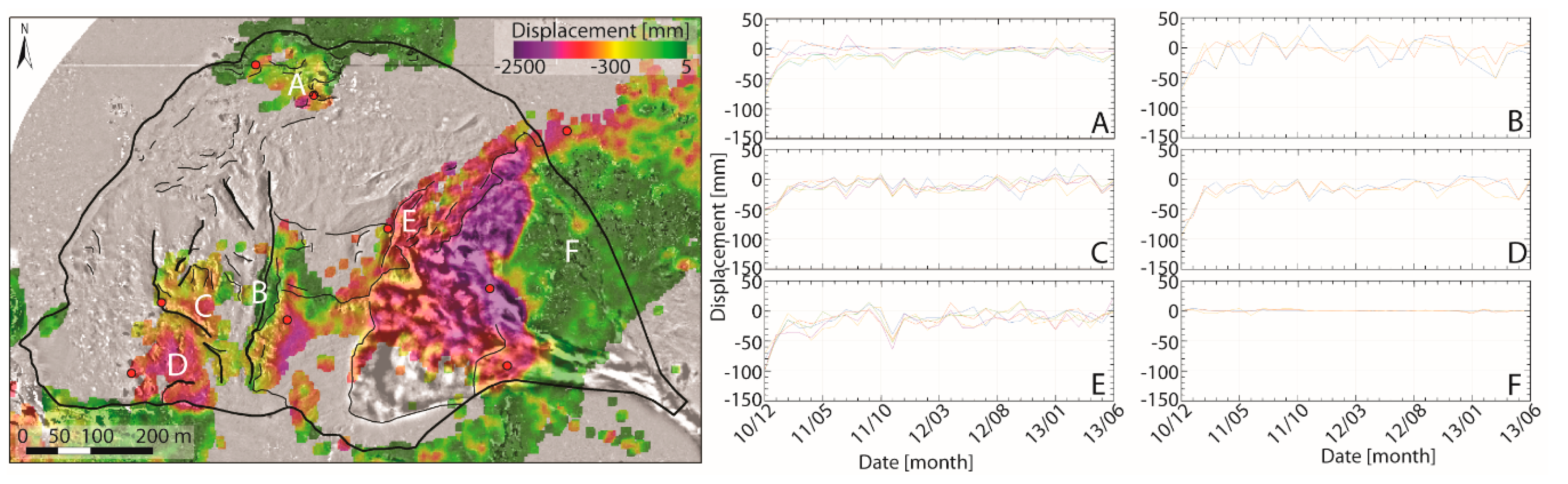According to the detailed geomorphological map [15], these areas were identified as follows:

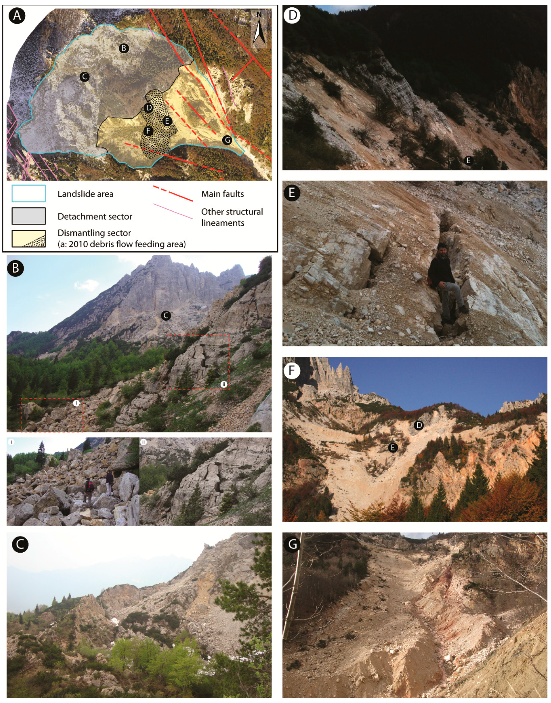
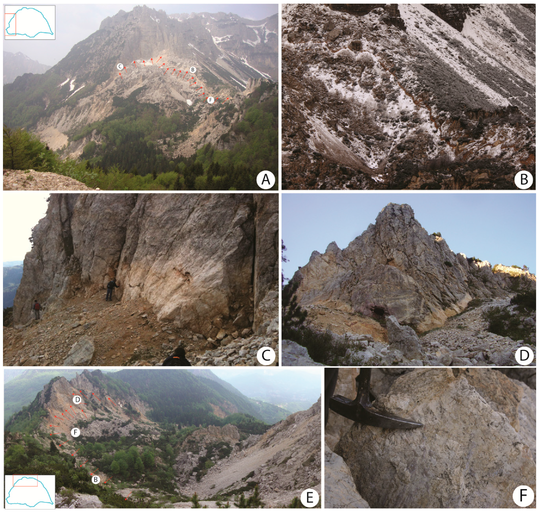
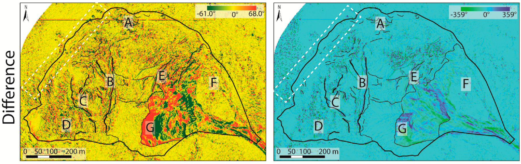
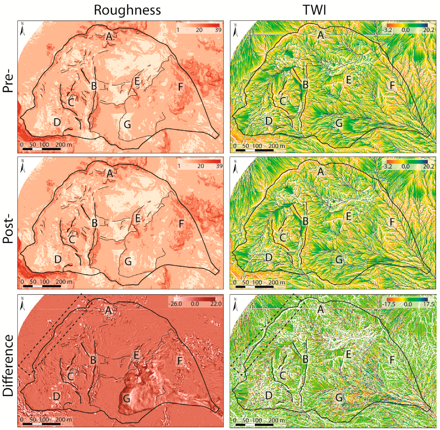
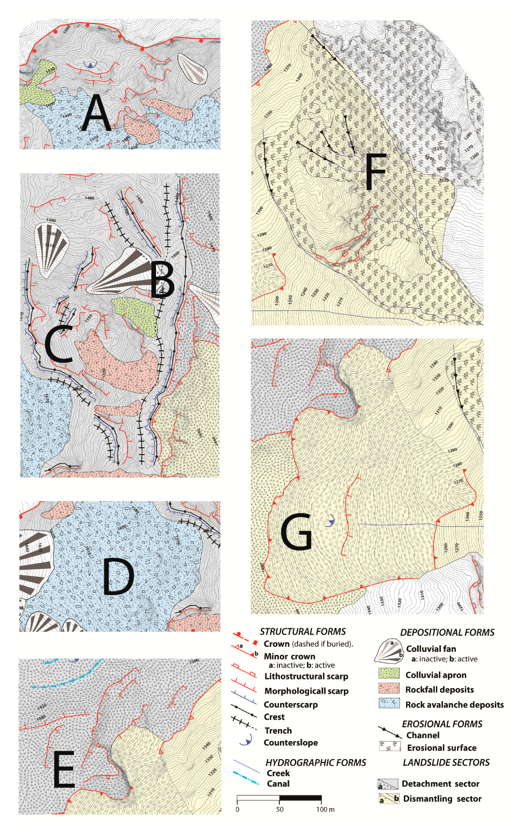
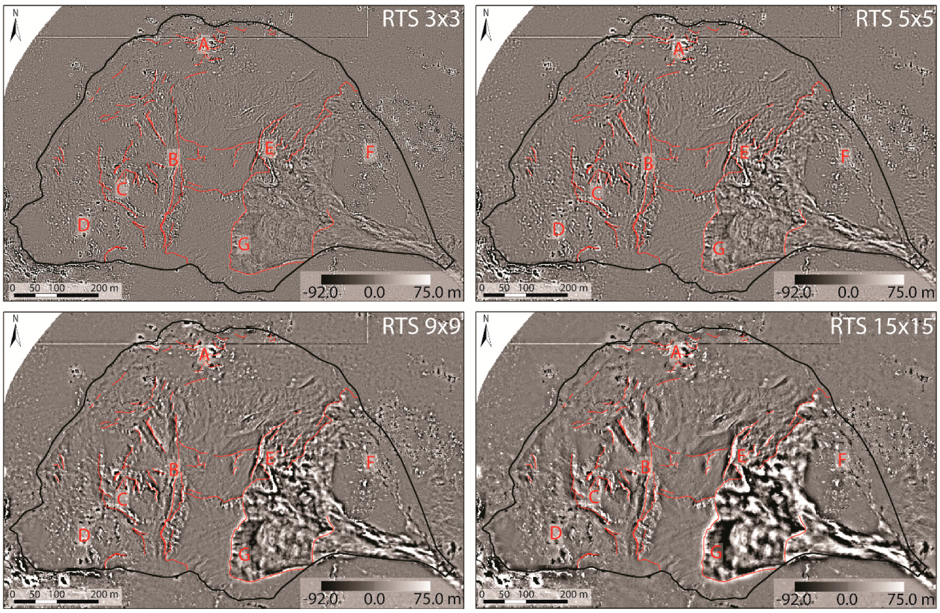
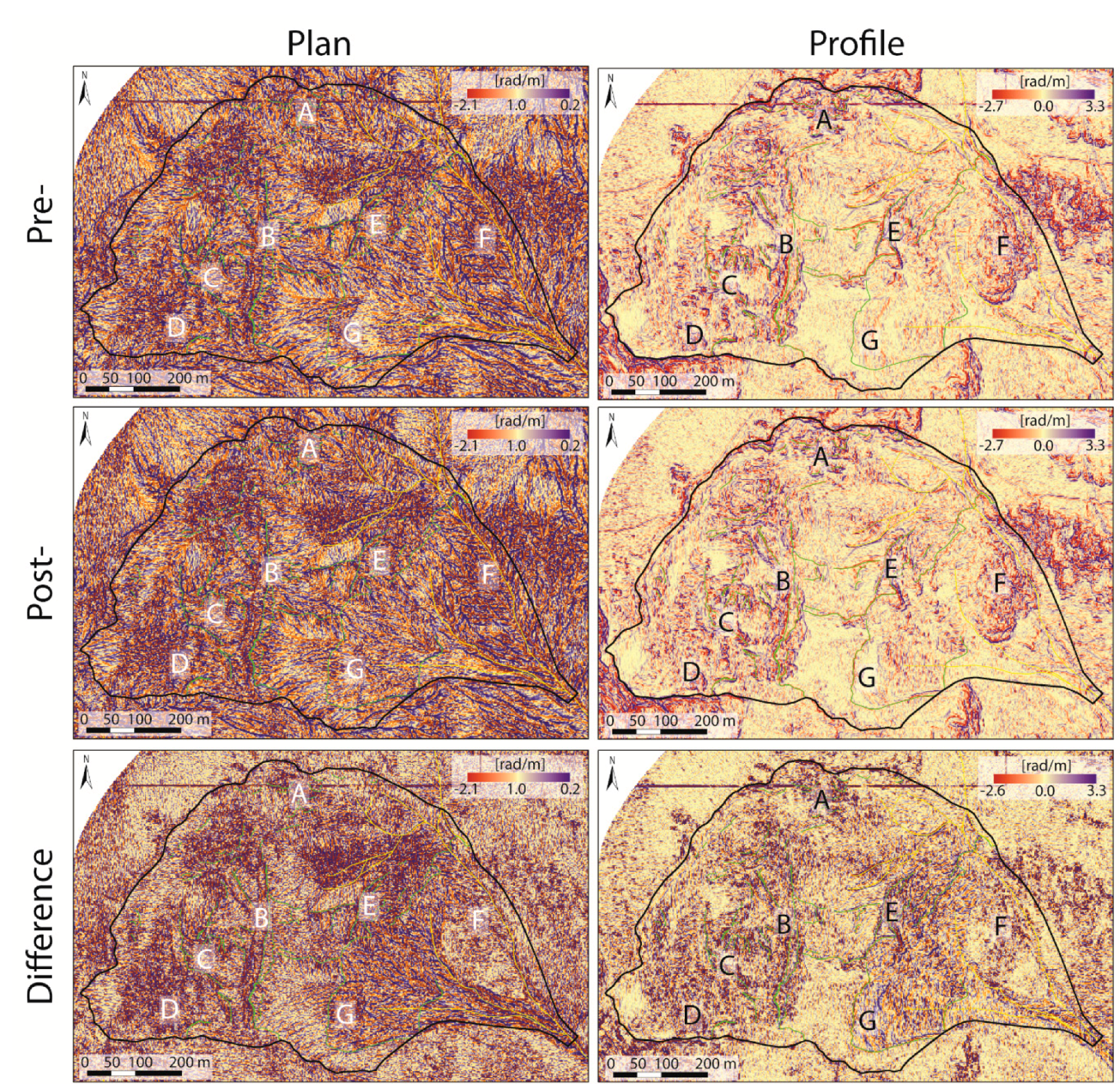
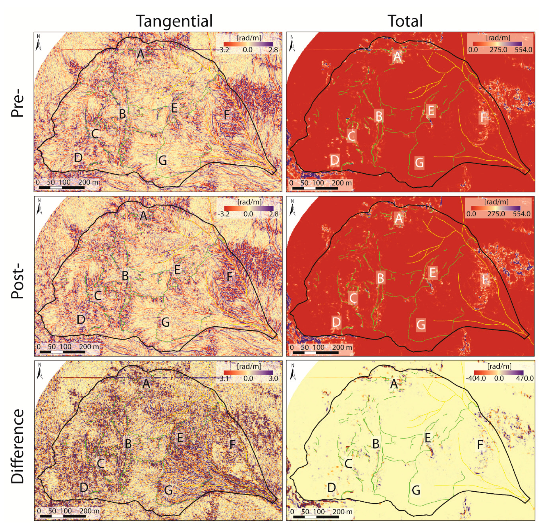
• A is the north portion of the landslide near the crown and is characterized by morphological scarps (Figure 7);
• B and C are in the west portion of the landslide and are characterized by scarps, counterscarps and trenches (Figure 7);
• D is in the south-west portion and is mainly characterized by rock avalanche deposits (Figure 7);
• E is in the middle-east portion between the detachment and the dismantling sectors, where there are the minor crow and morphological scarps (Figure 7); and
• F is in the east portion, in an area affected by erosional processes and characterized by lithostructural scarps (Figure 7).

The analysis of the difference maps (Figure 5 and Figure 6) showed that the variation in mean aspect is roughly −1.5°, whereas the mean slope variation is roughly −0.2°. Moreover, an anomaly (in the white dashed area in Figure 5 and Figure 6) at a mean distance from the main crown of approximately 20 m is evident in the slope, roughness, and TWI differences maps but not in the aspect differences map. This anomaly is associable with the newly activated 2010 sliding surface (Figure 3B) that changed the slope and surface roughness but did not affect the aspect.

The RTS maps were obtained by subtracting four different mean DEMs from the 2 m × 2 m DEMs created using the focal statistics ArcGIS tool with rectangular 3 × 3, 5 × 5, 9 × 9, and 15 × 15 cell moving windows. The RTS difference maps obtained by subtracting the post- and pre-RTS maps are shown in Figure 8. The six areas (A–F) characterized by higher variability are visible in all of the RTS difference maps, but the RTS15 × 15 map better highlights those differences and the newly activated 2010 sliding surface (highlighted with white arrows in Figure 8).

The hill shade maps (Figure 9) were obtained by simulating illumination from the north with altitude angles above the surface of the illumination source of 45° and 90°. The first simulation well illuminated the scarps, counterscarps and trenches in areas B and C and the rock avalanche deposits in D but shaded all the other areas that were brightened by the second simulation. The best results were obtained with the MDOW analysis that combined the results of the other two simulations, enhancing all the morphostructures that otherwise would have been shaded. Finally, the hill shade of the difference map clearly shows the six areas (A–F) affected by changes.

The plan (along the line of intersection between the surface and an XY plane) and profile (along the line of maximum slope, where the surface is intersected by the plane formed by the aspect and the Z-axis) curvatures are shown in Figure 10, and the tangential (along the line orthogonal to the line of steepest gradient) and total (general measure of the curvature of the surface itself, rather than the curvature of some line across the surface) curvatures of the pre- and post-DEMs and their differences are shown in Figure 11. Positive values of the plan and tangential curvatures describe how water would diverge as it flows over this point, and negative values show how it converges. Profile curvature describes how water would accelerate (negative values) or decelerate (positive values) flowing over a point, and total curvature is always positive and could be a measure of landscape ruggedness. The plan curvature has very low values except for the six areas (A–F), where the canals and the creeks north-west of area F and the morphostructures of the other areas are clearly recognizable. Canals and creeks are also well defined by the tangential curvature, which together with the profile curvature, shows a very complex situation over the entire landslide. The profile curvature well enhanced the morphostructures in the western part of area E. The pre- and post-total curvatures show that the main roughness is in the already defined six areas (A–F), and the difference map clearly shows that all these areas were affected by changes after the 2010 reactivation.

5. Discussion

Descriptions of the triggering or reactivation of DSGSD structures are usually associated with the development of extensive geomorphic structures expressed by distinguishable landscape morphologies, through which a typological classification [58] and degree of evolution [59] can be established. However, the entirety of slopes affected by DSGSDs generally can be differently deformed with millimetric-displacements [3,10] that often cannot be observed by means of field surveys. This can generate non-exhaustive safety awareness strategies in the risk management of these phenomena, which, on the contrary, often focus only on the more short-period localized hazardous effects (e.g., collateral debris flows). Therefore, a complete risk assessment strategy must also comprise the analysis of deep-seated impulsive phenomena. This type of behaviour can be observed effectively by using only high-resolution data obtained via advanced remote sensing techniques.

5.1. DSGSD Re-Activation

In the case study, the most undeniable evidence of the movement of the 2010 event was related to (i) a high mobile debris flow triggered from the debris cover of the lower sector (Figure 1 and Figure 2) and (ii) the appearance of a breaking/slip surface along the crown perimeter through a single impulse (Figure 3B). The first was an accessory and new occurrence that had evolutionary dynamics typical of rapid flow-like landslides, whereas the latter was a phenomenon linked to a deeper deformation that reactivated one of the main slip surfaces along the perimeter-breaking band. From the earliest post-event surveys, this rupture surface was immediately apparent, with a variable throw of some metres, to all the technicians who went up to check the status of the slopes. Despite the snow covering the entire area, it was possible to observe this fresh break continuously from one side of the border (Figure 3B) to the other, and at the same time, all of the geomorphological signs seemed to testify to an overall displacement of the mass. Therefore, the collection and analysis of high-resolution data based on advanced instrumentation were mandatory to obtain information that also pertained to the micro-morphological features descriptive of the event evolution. In this framework, the airborne remote imagery collected at a distance of a month (pre- and post-event) allowed the overall behaviour of the whole DSGSD to be detected during its re-activation.

The analysis of the DTM parameters (slope, aspect, surface roughness, hill shade, and curvature, Figure 5, Figure 6, Figure 8, Figure 9, Figure 10 and Figure 11) noted a regular change in morphology that can only be associated with laterally continuous short displacements along the maximum slope gradient. Despite the high masking worked by the accumulated rock blocks, each individual geomorphological domain developed homogeneous movements with a typical variation in shape and geometry on each known coordinate point. This slope evolution is mostly evident in the proximity of the major morphostructures such as the secondary crests, structural trenches, main scarps or tilted megablocks and in the land microforms of slopes tending to aggradation (detachment area) as well as those developing in protruding deformation (bulging area). In contrast, the same kind of spatial correlation does not run through pixels in the external area, and in some points, it even seems to be absent.

In the detachment area, they have a finely pronounced aspect but cover almost the whole area. Here, the existing fracturing system of the local carbonate rocks does not seem to have influenced the direction and velocity of downthrown movement, which resulted in a constant geometric deformation clearly represented by narrow parallel stripes in the comparative images of the surface geometrical properties. This is emblematic of ongoing large relaxing deformations that are being manifested, despite the high current stresses within the rock mass, here evidenced by some lineations (typical of fault mechanisms) discovered on the sliding surface between blocks in the central sector. The blocks we analysed are currently part of a dislocated system, but the orientation of the scratched lines along the dip direction remains consistent with the overall direction of the movement.

In the bulging area, deformations are more marked but are concentrated on the left slope immediately adjacent to the debris flow zone, behind a large stable rocky outcrop emerging from the sliding mass. The slope involved in the debris flow does not exhibit such morphologies, but during our inspections, some open high-angle macro fractures (Figure 2E) were identified for some metres in the outcropping bedrock, emerging in small isolated portions after the debris collapse. They are perpendicular to the inclination of the slope and constitute the most noticeable sign of the compressional character of the basal part of the DSGSD, which can give rise to the current high slopes (which are on average greater than those above) thanks to the action of the increasing bulging. The remaining slope immediately around them (such as the debris flow source area and the depositional path) have not developed other characterizing features due to the catastrophic nature of the collateral event, which concealed all of the deep evidence and did not allow, as elsewhere, linear morphologies related to the slow and controlled downward progression.

DoD analysis has been exploited in the literature to describe the 2010 debris flow event from the source area up to the distribution of the final deposit [16,36]. However, following the approach used in this work, the DoD (Figure 4) is useful to confirm the previous observations and in some cases to provide additional supporting evidence. The distribution of the information reported by each pixel, which at first sight can be confused with an error descended from the original processing or at least local accidents, reflects the same alternating geometric texture of the previously discussed displacements for the entire mobilized DSGSD, even if in a less obvious way from a visual point of view. The incidence of the system of these dense bands is particularly evident in the detachment area and can be associated with an alternating sequence of the loss and appearance of material over a point (vertical variation due to the advancing landslide).

In Figure 12, morphological and altitude variations along five cross sections show the local effect of the down-sliding, which assumes the abovementioned parallel forms if viewed from above. In the bulging area, the removal (red areas in Figure 12A and blue areas in Figure 12B) and storage zones (blue areas in Figure 12A and red areas in Figure 12B) are more persistent and continuous. On the DSGSD right flank, a removal zone is present in the upper portion (the large red area in Figure 12A associated with the 2010 debris flow), and just at its foot a storage zone (the debris flow deposition area shown in Figure 1) develops up to the narrow valley floor (the elongated blue strip in Figure 12). Throughout this zone, the deep-seated dislocations analysed using the differential DEM were masked by intense displacements caused by the 2010 debris flow detachment (enlargements 1 and 2 in Figure 12C); therefore, no evidence of surface microvariations is present in any of the elaborated maps (Figure 5, Figure 6, Figure 8, Figure 9, Figure 10 and Figure 11). In contrast, on the left adjacent side, a large storage zone is present (enlargements 3 and 4 in Figure 12), again without bend shapes. We believe that this positive deformation was not caused by a debris accumulation after a collapse because any detachment area exists upstream. Further, given the existing high slopes, it is highly unlikely that a material accumulation can come from the mobilized detritus through horizontal sliding. Therefore, considering this landslide context, the thick detrital cover was pushed forward in a significant component by the deep-seated deformation during the bulging evolution of the bedrock. In this case, differently from the adjacent area, the conditions for the break did not occur, and the material remained hanging on the slope. Consequently, the present aspect of a part of this landscape is apparently dominated by surface processes that mask deeper evolutionary phenomena (Figure 4C). The volume gain and loss of the whole landslide are summarized in

Table 1. Positive (Loss—removed material) and negative (Gain—accumulation) volume variations.

Calculated Features	Total	Detachment Sector	Bulging Sector
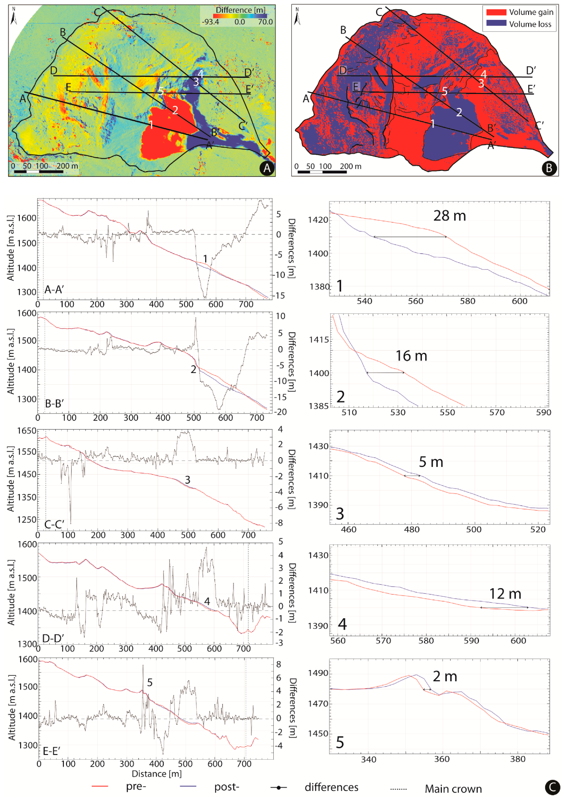
Volume gain [m3]	−232,942.0	−231,644.0	−216,543.0
Area [%]	55.9	58.0	54.0
Volume loss [m3]	411,059.0	402,021.0	404,250.0
Area [%]	44.0	42.0	46.0
Volume variation [m3]	178,117.0	170,377.0	187,707.0
2010 debris flow volume [m3]	-	-	322,220.0

.

A further sign of the expansive deformation of this area can also be identified over almost two megablocks in zone E (1 and 2 in Figure 4), which have tilted alignments (anti-dip slopes) with respect to the horizontal orientation of stable rocks all around the DSGSD. During the reactivation, their feet were disentangled by the 2010 debris flow occurrence, but at the same time, the whole of the rock masses continued their historical roto-translation evolution, expressing a positive mass balance just where the opposite consequence would be expected for rapid and strong detritus removal. However, as noted even by field inspections, no new material deriving from the above slopes moved and contributed to this volume budget.

5.2. DSGSD Residual Movements

The GB-InSAR acquisition started approximately two weeks after the DSGSD reactivation, and from that moment on, it allowed monitoring of the residual deformations over the main geomorphological structures. Such instrumental observations were carried out from December 2010 to June 2013, with special attention to sectors where the radar signal was characterized by high stability (details in [18]). Immediately after the beginning of the monitoring, all the areas that showed signs of deep displacement during the reactivation again proved to be particularly active some weeks later. The main movements continued until February 2011, and subsequently, depending on the concerned morphostructures, they decreased to minimum values throughout the whole observation period, testifying the slow downloading of inner forces that began with the impulsive advance of 4 November 2010 (Figure 13). Only the suspended debris below zone E had a different evolution. Movements there continued significantly throughout the period, with alternating stages of progression, and reached a maximum displacement of 2437 mm. These movements were mainly concentrated in a narrow portion of slope comprising a canal in which an ephemeral creek sometimes seasonally appears. Unlike the other cases in this circumstance, the moving mass centre shifted slowly over time (without accelerations or rapid landslide triggers) from the highest slope to the bottom. Therefore, the evolutionary dynamics of this sector can be associated with both the deeper structural deformation and surface dismantling action concerning the debris cover rearrangement, but in virtue of the development process, it is impossible to separate the two components using uniquely radar data. However, these deep and slow thrusts mobilizing residual loose material and transferring the barycentre were insufficient to trigger new collapses despite the occurrence of precipitations comparable to those in 2010, and they were limited to aiding the material find new balances over high slopes. To date, no debris flows have yet occurred from this critical slope.

6. Conclusions

The kinematic behaviour of the Rotolon DSGSD reactivation after the October–November 2010 rainfalls has been presented in this paper by means of the analysis of two LiDAR derived DEMs and their parameters. Employing a metaheuristic approach, it was found that the 2010 event apparently was limited to secondary and localized phenomena such as debris flows in the bulging area, without direct reactivation clues, other than the presence of a continuous perimeter fracture associated with the crown area. The analysis of the DEM parameters noted not only shallower movements in the bulging area but also regular morphological changes throughout the landslide that were connected with deeper continuous displacements along the maximum slope gradient, thus confirming the DSGSD reactivation. Moreover, the displacements connected to the DSGSD reactivation did not cease immediately, particularly far from the break/crown zone (as shown by the GB-InSAR analysis), but continued with very slow deformations until the new equilibrium was reached, testifying to the impulsive behaviour of the landslide.

References

- Dramis, F.; Farabollini, P.; Gentili, P.; Pambianchi, G. Neotectonis and large-scale gravitational phenomena in the Umbria-Marche Apennines, Italy. In Steepland Geomorphology; Slaymaker, O., Ed.; J. Wiley & Sons: Chichester, UK, 1995; pp. 199–217. [Google Scholar]
- Hippolyte, J.C.; Brocard, G.; Tardy, M.; Nicoud, G.; Bourlès, D.; Braucher, R.; Ménard, G.; Souffaché, B. The recent fault scarps of the Western Alps (France): Tectonic surface ruptures or gravitational sackung scarps? A combined mapping, geomorphic, levelling, and 10Be dating approach. Tectonophysics 2006, 418, 255–276. [Google Scholar] [CrossRef]
- Agliardi, F.; Crosta, G.B.; Frattini, P. Slow rock-slope deformation. In Landslide: Types, Mechanisms and Modelling, 1st ed.; Clague, J.J., Stead, D., Eds.; Cambridge University Press: New York, NY, USA, 2012; pp. 207–221. ISBN 9781107002067. [Google Scholar]
- Crosta, G.B.; Agliardi, F.; Frattini, P. Deep seated gravitational slope deformations in the European Alps. Tectonophysics 2013, 605, 13–33. [Google Scholar] [CrossRef]
- Cruden, D.M.; Varnes, D.J. Landslide types and processes. In Landslides: Investigation and Mitigation; Turner, A.K., Shuster, R.L., Eds.; Transportation Research Board: Washington, DC, USA, 1996; pp. 36–75. [Google Scholar]
- Ambrosi, C.; Crosta, G.B. Large sackung along major tectonic features in the Central Alps. Eng. Geol. 2006, 83, 183–200. [Google Scholar] [CrossRef]
- Zischinsky, U. On the deformation of high slopes. In Proceedings of the First Conference of the International Society for Rock Mechanics, Lisbon, Portugal, 25 September–1 October 1966; Volume 2, pp. 179–185. [Google Scholar]
- Hutchinson, J.N. General Report: Morphological and geotechnical parameters of landslides in relation to geology and hydrogeology. In Proceedings of the 5th International Symposium on Landslides, Lausanne, Switzerland, 10–15 July 1988; Volume I, pp. 3–35. [Google Scholar]
- Bovis, M. Rock-slope deformation at Affliction Creek, southern Coast Mountains, British Columbia. Can. J. Earth Sci. 1990, 27, 243–254. [Google Scholar] [CrossRef]
- Agliardi, F.; Crosta, G.B.; Zanchi, A. Structural constraints on deep-seated slope deformation kinematics. Eng. Geol. 2001, 59, 83–102. [Google Scholar] [CrossRef]
- Jaboyedoff, M.; Penna, I.; Pedrazzini, A.; Baroň, I.; Crosta, G.B. An introductory review on gravitational-deformation induced structures, fabrics and modelling. Tectonophysics 2013, 605, 1–12. [Google Scholar] [CrossRef]
- McCalpin, J.P.; Irvine, J.R. Sackungen at Aspen Highlands Ski Area, Pitkin County, Colorado. Environ. Eng. Geosci. 1995, 1, 277–290. [Google Scholar] [CrossRef]
- Varnes, D.J.; Radbruch-Hall, D.; Savage, W.Z. Topographic and structural conditions in areas of gravitational spreading of ridges in the western United States. U. S. Geol. Surv. Prof. Pap. 1989, 1496, 1–28. [Google Scholar]
- Pánek, T.; Klimeš, J. Temporal behavior of deep-seated gravitational slope deformation: A review. Earth Sci. Rev. 2016, 156, 14–38. [Google Scholar] [CrossRef]
- Frodella, W.; Morelli, S.; Fidolini, F.; Pazzi, V.; Fanti, R. Geomorphology of the Rotolon landslide (Veneto region, Italy). J. Maps 2014, 10, 394–401. [Google Scholar] [CrossRef]
- Salvatici, T.; Morelli, S.; Pazzi, V.; Frodella, W.; Fanti, R. Debris flow hazard assessment by means of numerical simulations: Implications for the Rotolon Creek Valley (Northern Italy). J. Mt. Sci. 2017, 14, 636–648. [Google Scholar] [CrossRef]
- Zangerl, C.; Eberhardt, E.; Perzlmaier, S. Kinematic behaviour and velocity characteristics of a complex deep-seated crystalline rockslide system in relation to its interaction with a dam reservoir. Eng. Geol. 2010, 112, 53–67. [Google Scholar] [CrossRef]
- Frodella, W.; Morelli, S.; Pazzi, V. Infrared thermographic surveys for landslide mapping and characterization: The Rotolon DSGSD (Northern Italy) case study. Int. J. Eng. Geol. Environ. 2017, 1, 77–84. [Google Scholar] [CrossRef]
- Kasai, M.; Ikeda, M.; Asahina, T.; Fujisawa, K. LiDAR-derived DEM evaluation of deep-seated landslides in a steep and rocky region of Japan. Geomorphology 2009, 113, 57–69. [Google Scholar] [CrossRef]
- Crosta, G.B.; di Prisco, C.; Frattini, P.; Frigerio, G.; Castellanza, R.; Agliardi, F. Chasing a complete understanding of the triggering machanisms of a large rapidly evolving rockslide. Landslides 2014, 11, 747–764. [Google Scholar] [CrossRef]
- Barla, G.; Antolini, F.; Barla, M.; Mensi, E.; Piovano, G. Monitoring of the Beauregard landslide (Aosta Valley, Italy) using advanced and conventional techniques. Eng. Geol. 2010, 116, 218–235. [Google Scholar] [CrossRef]
- Frigerio, S.; Schenato, L.; Bossi, G.; Cavalli, M.; Mantovani, M.; Marcato, G.; Pasuto, A. A web-based platform for automatic and continuous landslide monitoring: The Rotolon (Eastern Italian Alps) case study. Comput. Geosci. 2014, 63, 96–105. [Google Scholar] [CrossRef]
- Casagli, N.; Frodella, W.; Morelli, S.; Tofani, V.; Ciampalini, A.; Intrieri, E.; Raspini, F.; Rossi, G.; Tanteri, L.; Lu, P. Spaceborne, UAV and ground-based remote sensing techniques for landslide mapping, monitoring and early warning. Geoenviron. Disasters 2017, 4, 9. [Google Scholar] [CrossRef]
- Casagli, N.; Tofani, V.; Morelli, S.; Frodella, W.; Ciampalini, A.; Raspini, F.; Intrieri, E. Remote sensing techniques in Landslide Mapping and Monitoring, Keynote Lecture. In Advancing Culture of Living with Landslides; Mikos, M., Arbanas, Ž., Yin, Y., Sassa, K., Eds.; Advances in Landslide Technology; Springer International Publishing: Cham, Switzerland, 2017; Volume 3, pp. 1–19. [Google Scholar]
- Frodella, W.; Salvatici, T.; Pazzi, V.; Morelli, S.; Fanti, R. GB-InSAR monitoring of slope deformations in a mountainous area affected by debris flow events. Nat. Hazards Earth Syst. Sci. 2017, 17, 1779–1793. [Google Scholar] [CrossRef]
- Pazzi, V.; Lotti, A.; Chiara, P.; Lombardi, L.; Nocentini, M.; Casagli, N. Monitoring of the vibration induced on the Arno masonry embankment wall by the conservation works after the 25 May 2016 riverbank landslide. Geoenviron. Disasters 2017, 4, 6. [Google Scholar] [CrossRef]
- Fidolini, F.; Pazzi, V.; Frodella, W.; Morelli, S.; Fanti, R. Geomorphological characterization, monitoring and modeling of the Monte Rotolon complex landslide (Recoaro terme, Italy). In Engineering Geology for Society and Territory—Volume 2; Lollino, G., Giordan, D., Crosta, G., Corominas, J., Azzam, R., Wasowski, J., Sciarra, N., Eds.; Springer International Publishing: Cham, Switzerland, 2015; pp. 1311–1315. [Google Scholar]
- Jaboyedoff, M.; Oppikofer, T.; Abellán, A.; Derron, M.H.; Loye, A.; Metzger, R.; Pedrazzini, A. Use of LIDAR in landslide investigations: A review. Nat. Hazards 2012, 61, 5–28. [Google Scholar] [CrossRef]
- Lotti, A.; Saccorotti, G.; Fiaschi, A.; Matassoni, L.; Gigli, G.; Pazzi, V.; Casagli, N. Seismic monitoring of rockslide: The Torgiovannetto quarry (Central Apennines, Italy). In Engineering Geology for Society and Territory—Volume 2; Lollino, G., Giordan, D., Crosta, G., Corominas, J., Azzam, R., Wasowski, J., Sciarra, N., Eds.; Springer International Publishing: Cham, Switzerland, 2015; pp. 1537–1540. [Google Scholar]
- Pazzi, V.; Tapete, D.; Cappuccini, L.; Fanti, R. An electric and electromagnetic geophysical approach for subsurface investigation of anthropogenic mounds in an urban environment. Geomorphology 2016, 273, 335–347. [Google Scholar] [CrossRef]
- Pazzi, V.; Tanteri, L.; Bicocchi, G.; D’Ambosio, M.; Caselli, A.; Fanti, R. H/V measurements as an effective tool for the reliable detection of landslide slip surfaces: Case studies of Castagnola (La Spezia, Italy) and Roccalbegna (Grosseto, Italy). Phys. Chem. Earth 2017, 98, 136–153. [Google Scholar] [CrossRef]
- Frodella, W.; Fidolini, F.; Morelli, S.; Pazzi, V. Application of Infrared Thermography for landslide mapping: The Rotolon DSGDS case study. Rend. Online Soc. Geol. Ital. 2015, 35, 144–147. [Google Scholar] [CrossRef]
- Cola, S.; Bossi, G.; Munari, S.; Brezzi, L.; Marcato, G. Applicability of two propagation models to simulate the Rotolon earth-flow occurred in November 2010. In Engineering Geology for Society and Territory—Volume 2; Lollino, G., Giordan, D., Crosta, G., Corominas, J., Azzam, R., Wasowski, J., Sciarra, N., Eds.; Springer International Publishing: Cham, Switzerland, 2015; pp. 1683–1687. [Google Scholar]
- Trivelli, G. Storia del Territorio e Delle Genti di Recoaro; Istituto Geografico De Agostini: Novara, Italy, 1991; p. 256. (In Italian) [Google Scholar]
- Altieri, V.; Colombo, P.; Dal Prà, A. Studio per la Valutazione Delle Condizioni di Stabilità dei Versanti e del Fondovalle del Bacino Idrografico del Torrente Rotolon nell’Alta Valle dell’Agno in Comune di Recoaro Terme (Vicenza). Relazione Geologico—Geotecnica; Regione del Veneto Segreteria Regionale per il Territorio—Dipartimento Lavori Pubblici: Venezia, Italy, 1994; p. 97. (In Italian) [Google Scholar]
- Bossi, G.; Cavalli, M.; Crema, S.; Frigerio, S.; Quan Luna, B.; Mantovani, M.; Marcato, G.; Schenato, L.; Pasuto, A. Multi-temporal LiDAR-DTMs as a tool for modelling a complex landslide: A case study in the Rotolon catchment (eastern Italian Alps). Nat. Hazards Earth Syst. Sci. 2015, 15, 715–722. [Google Scholar] [CrossRef]
- Schneuwly-Bollschweiler, M.; Stoffel, M.; Rudolf-Miklau, F. Dating Torrential Processes on Fans and Cones: Methods and Their Application for Hazard and Risk Assessment; Springer: London, UK, 2012; p. 423. ISBN 978-94-007-4336-6. [Google Scholar]
- Gigli, G.; Morelli, S.; Fornera, S.; Casagli, N. Terrestrial laser scanner and geomechanical surveys for the rapid evaluation of rock fall susceptibility scenarios. Landslides 2014, 11, 1–14. [Google Scholar] [CrossRef]
- Gigli, G.; Frodella, W.; Garfagnoli, F.; Morelli, S.; Mugnai, F.; Menna, F.; Casagli, N. 3-D geomechanical rock mass characterization for the evaluation of rockslide susceptibility scenarios. Landslides 2014, 11, 131–140. [Google Scholar] [CrossRef]
- Del Soldato, M.; Segoni, S.; De Vita, P.; Pazzi, V.; Tofani, V.; Moretti, S. Thickness model of pyroclastic soils along mountain slopes of Campania (southern Italy). In Landslides and Engineered Slopes. Experience, Theory and Practice; Aversa, S., Cascini, L., Picarelli, L., Scavia, C., Eds.; Associazione Geotecnica Italaiana: Rome, Italy, 2016; pp. 797–804. ISBN 978-1-138-02988-0. [Google Scholar]
- Morelli, S.; Pazzi, V.; Monroy, V.H.G.; Casagli, N. Residual slope stability in low order streams of Angangueo mining area (Michoacán, Mexico) after the 2010 debris flows. In Advancing Culture of Living with Landslides; Mikos, M., Casagli, N., Yin, Y., Sassa, K., Eds.; Volume 4—Diversity of Landslide Forms; Springer International Publishing: Cham, Switzerland, 2017; pp. 651–660. [Google Scholar]
- Pazzi, V.; Tanteri, L.; Bicocchi, G.; Caselli, A.; D’Ambosio, M.; Fanti, R. H/V technique for the rapid detection of landslide slip surface(s): Assessment of the optimized measurements spatial distribution. In Advancing Culture of Living with Landslides; Mikos, M., Tiwari, B., Yin, Y., Sassa, K., Eds.; Volume 2—Advances in Landslide Science; Springer International Publishing: Cham, Switzerland, 2017; pp. 335–343. [Google Scholar]
- Pazzi, V.; Morelli, S.; Fidolini, F.; Krymi, E.; Casagli, N.; Fanti, R. Testing cost-effective methodologies for flood and seismic vulnerability assessment in communities of developing countries (Dajç northern Albania). Geomat. Nat. Hazards Risk 2016, 7, 971–999. [Google Scholar] [CrossRef]
- Pazzi, V.; Morelli, S.; Pratesi, F.; Sodi, T.; Valori, L.; Gambacciani, L.; Casagli, N. Assessing the safety of schools affected by geo-hydrologic hazards: The geohazard safety classification (GSC). Int. J. Disaster Risk Reduct. 2016, 15, 80–93. [Google Scholar] [CrossRef]
- Evans, I. General geomorphometry. In Geomorphological Techniques, 2nd ed.; Goudie, A., Ed.; Routledge Taylor & Francis Group: New York, NY, USA, 1990; pp. 49–62. ISBN 0-415-11939-1. [Google Scholar]
- Li, Z.; Zhu, Q.; Gold, C. Digital Terrain Modeling—Principles and Methodology; CRC Press: Boca Raton, FL, USA, 2005; p. 319. ISBN 0-415-32462-9. [Google Scholar]
- Kasprzak, M.; Duszyñski, F.; Jancewicz, K.; Michniewicz, A.; Rózycka, M.; Migoñ, P. The Rogowiec Landslide Complex (Central Sudetes, SW Poland)—A case of a collapsed mountain. Geol. Q. 2016, 60, 695–713. [Google Scholar] [CrossRef]
- Jenness, J. DEM Surface Tools for ArcGIS (surface_area.exe). 2013. Jenness Enterprises. Available online: http://www.jennessent.com/arcgis/surface_area.htm (accessed on 9 November 2017).
- Cavalli, M.; Marchi, L. Characterisation of the surface morphology of an alpine alluvial fan using airbone LiDAR. Nat. Hazards Earth Syst. Sci. 2008, 8, 323–333. [Google Scholar] [CrossRef]
- Sørensen, R.; Zinko, U.; Seibert, J. On the calculation of the topographic wetness index: Evaluation of di erent methods based on field observations. Hydrol. Earth Syst. Sci. 2006, 10, 101–112. [Google Scholar] [CrossRef]
- Fleming, M.D.; Hoffer, R.M. Machine Processing of Landsat MSS Data and DMA Topographic Data for Forest Cover Type Mapping; LARS Technical Report 062879; Laboratory for Applications of Remote Sensing, Purdue University: West Lafayette, IN, USA, 1979; p. 17. [Google Scholar]
- Jones, K.H. A comparison of algorithms used to compute hill slope as a property of the DEM. Comput. Geosci. 1998, 24, 315–323. [Google Scholar] [CrossRef]
- Jenness, J. Calculating landscape surface area from digital elevation model. Wildl. Soc. Bull. 2004, 32, 829–839. [Google Scholar] [CrossRef]
- Mark, R. A Multidirectional, Oblique-Weighted, Shaded-Relief Image of the Island of Hawaii; U.S. Geological Survey Open-File Report 92.422; U.S. Geological Survey: Reston, VA, USA, 1992.
- Cavalli, M.; Tarolli, P.; Marchi, L.; Dalla Fontana, G. The effectiveness of airborne LiDAR data in the recognition of channel-bed morphology. Catena 2008, 7, 249–260. [Google Scholar] [CrossRef]
- Ventura, G.; Vilardo, G.; Terranova, C.; Bellucci Sessa, E. Trackong and evolution of complex active landslide by multi-temporal airborne LiDAR data: The Montaguto landslide (Southern Italy). Remote Sens. Environ. 2011, 115, 3237–3248. [Google Scholar] [CrossRef]
- Tarchi, D.; Ohlmer, E.; Sieber, A.J. Monitoring of structural changes by radar interferometry. Res. Nondestruct. Eval. 1997, 9, 213–225. [Google Scholar] [CrossRef]
- Schleier, M.; Hermanns, R.L.M.; Krieger, I.; Oppikofer, T.; Eiken, T.; Rønning, J.S.; Rohn, J. Gravitational reactivation of a pre-existing post-Caledonian fault system: The deep-seated gravitational slope deformation at Middagstinden, western Norway. Nor. J. Geol. 2016, 96, 1–23. [Google Scholar] [CrossRef]
- Borrelli, L.; Gullà, G. Tectonic constraints on a deep-seated rock slide in weathered crystalline rocks. Geomorphology 2017, 290, 288–316. [Google Scholar] [CrossRef]