Article

Landslide Change Detection Based on Multi-Temporal Airborne LiDAR-Derived DEMs

by
Omar E. Mora
1,*,
M. Gabriela Lenzano
2,
Charles K. Toth
3,
Dorota A. Grejner-Brzezinska
3 and
Jessica V. Fayne
4
1
Civil Engineering Department, California State Polytechnic University, Pomona, Pomona, CA 91768, USA
2
Instituto Argentino de Nivología, Glaciología y Ciencias Ambientales (IANIGLA)—CONICET, 5500 Mendoza, Argentina
3
Department of Civil, Environmental and Geodetic Engineering, The Ohio State University, Columbus, OH 43210, USA
4
Department of Geography, University of California, Los Angeles, CA 90095, USA
*
Author to whom correspondence should be addressed.
Geosciences 2018, 8(1), 23; https://doi.org/10.3390/geosciences8010023
Submission received: 5 December 2017 / Revised: 10 January 2018 / Accepted: 13 January 2018 / Published: 16 January 2018
(This article belongs to the Special Issue Natural Hazards and Risks Assessment)

Abstract

:
Remote sensing technologies have seen extraordinary improvements in both spatial resolution and accuracy recently. In particular, airborne laser scanning systems can now provide data for surface modeling with unprecedented resolution and accuracy, which can effectively support the detection of sub-meter surface features, vital for landslide mapping. Also, the easy repeatability of data acquisition offers the opportunity to monitor temporal surface changes, which are essential to identifying developing or active slides. Specific methods are needed to detect and map surface changes due to landslide activities. In this paper, we present a methodology that is based on fusing probabilistic change detection and landslide surface feature extraction utilizing multi-temporal Light Detection and Ranging (LiDAR) derived Digital Elevation Models (DEMs) to map surface changes demonstrating landslide activity. The proposed method was tested in an area with numerous slides ranging from 200 m2 to 27,000 m2 in area under low vegetation and tree cover, Zanesville, Ohio, USA. The surface changes observed are probabilistically evaluated to determine the likelihood of the changes being landslide activity related. Next, based on surface features, a Support Vector Machine (SVM) quantifies and maps the topographic signatures of landslides in the entire area. Finally, these two processes are fused to detect landslide prone changes. The results demonstrate that 53 out of 80 inventory mapped landslides were identified using this method. Additionally, some areas that were not mapped in the inventory map displayed changes that are likely to be developing landslides.

1. Introduction

Fast-moving soil slip-debris flows triggered by natural phenomena are often destructive, causing widespread damage and environmental change. Each type of slope movement poses different threat levels and may require a separate assessment based on the distinct definitions of a landslide [1]. The factors and basis of landslides vary, and the impact of landslides are well known, but the knowledge and study of each case must be optimized to provide the best solution for a specific region (e.g., [2,3,4,5]). Landslide analysis and mapping can provide the locations of previous events as well as indicate the probable locations of future events. Landslide event maps are categorized by regional or potential landslides, and site-specific information that helps regulate danger and risk. Determining the spatial extent of landslide threats requires inventory of those areas, and these maps can provide essential information for the prevention of potential damages through planning and decision making [2,6,7,8].
Remote sensing techniques have been used to measure surface processes by conducting change detection for volumetric change such as map erosion and deposition (e.g., [9,10,11,12]). Geomorphologic analysis for landslide terrains has consisted of field observation, airborne LiDAR, traditional surveying, global positioning system (GPS), aerial photograph interpretation, or a combination of these techniques ([13,14,15,16,17,18,19,20]). Improvements made in remote sensing technology provide new opportunities to map surface models precisely and accurately at spatial resolutions and temporal frequencies necessary for landslide mapping of small failures in open areas and under most land cover conditions such as fields and sparse forests. Newer change detection techniques for landslide mapping in large swaths of terrain are based on object-oriented methods that typically use optical imagery [21,22]. These methods have proven to be useful for mapping landslide events through object-oriented segment-based classification. However, these methods are incapable of mapping surface deformations of small failures under canopy cover. Because of problems of scale of the available data, current techniques focus on large landslides, active slides and catastrophic events (e.g., [23,24,25]). Conversely, less attention is paid to modestly deforming, small failures that continuously impact our infrastructure that require higher spatial resolution data [26,27].
In 1994, Ref. [9] introduced repeat topographic surveys to produce Digital Elevation Model (DEM) of Difference (DoD) maps by a rigorous comparison of analytically derived photogrammetric DEM product with ground survey. The ability to observe surface deformation from change detection on DEMs presented a new opportunity to identify, predict and quantify landslides [28]. DoD maps have become important in landslide mapping where vertical changes reflect the spatial and temporal processes of landslides. DoD maps are highly effective means to monitor temporal changes when change calculations have accounted for measurement uncertainties [10,11,12]. In addition it is essential that DEM generation and multi-temporal registration be performed appropriately [12].
Presently, LiDAR technology is the most effective approach for high-density and high-accuracy three-dimensional terrain point data acquisition; one of the advantages is the direct availability of three-dimensional coordinates of points in object space with up to sub-decimeter accuracy, offering the most accurate surface elevation information for natural event monitoring by DEMs [23,24,29,30]. Also, LiDAR offers an optimal solution to reduce the amount of field investigation necessary to identify and monitor landslide changes under open and canopy-covered terrain.
In this paper, we propose a method that fuses change detection and supervised classification based on LiDAR data that can be used to prevent potential risk associated with landslides and those provided in a landslide inventory. The corridor of State Route (SR) 666 in Zanesville, Ohio was used as a test area to assess the performance of the proposed method. The study contributes to the detection of temporal changes caused by small landslides. The outline of this paper is as follows: Section 2 provides a detailed review of the study area, data set employed including uncertainty calculation, and landslide inventory used as ground truth. Section 3 reviews the three-part landslide detection methodology using probabilistic change detection, landslide surface feature extraction using a supervised classifier, and landslide detection. Section 4 presents a detailed analysis of the results and, finally, Section 5 includes a discussion and conclusion of the proposed method.

2. Area Description and Data Setting

2.1. Study Area

The study area is the transportation corridor of SR 666 in Zanesville, Ohio, located in north-central Muskingum County (Approx. Latitude: N 39°58′00″, Longitude: W 81°59′00″) east of the Muskingum River. The study area begins within the City of Zanesville and ends east of the Village of Dresden. The extent of the study area is 23 km in length along SR 666 with a varying swath of 75–180 m. The area is characterized by dense vegetation, stream and river channeling, some residential development and post-mining activity in sloped terrain. The study area was selected due to its prolonged history of slope instabilities particularly in areas where the river is near the roadway. Along the road, seven separate sections were damaged by landslides as a result of storm events in 2004 and 2005. Figure 1 presents an overview map of the study area. The availability of multi-temporal DEMS and landslide inventory map make this an ideal case to study the utility of extracting landslide features using probabilistic change detection with supervised classification.
The study area is located within the Muskingum-Pittsburgh Plateau Physiographic Region which is located within the Unglaciated Allegheny Plateaus of the Appalachian Plateaus Section. Characteristics of the Muskingum-Pittsburgh Plateau Physiographic Region are broad major drainage valleys that contain glacial outwash deposits and lacustrine terraces surrounded by moderate to high relief. Within the study area, topographic relief ranges from 61 to 122 m (200 to 400 feet) from the Muskingum River to the hilltops just east of the river. The valley walls of the Muskingum River within the project area are characterized by very steep quickly dropping bedrock faces as a result of scouring and erosion by the river. At the inside bends of the river, the soil overburden ranges from minimal <1.52 m (<5 feet) to very thick >15.24 m (>50 feet) overlying the scoured bedrock surface and are dependent upon the location of the road. The six primary soil types found within the study area consists of alluvium, glacial outwash, lacustrine soils, colluvium, residual soils, and man-made fill. Berks-Westmoreland complex (Bkf) soil found in 40 to 70 percent slopes was the soil type for approximately 92 percent of the mapped landslides in our study area. Bkf has the most rugged terrain in the county and it is common to see unstable slopes in this soil type, in addition, the soil has a severe hazard of erosion. Bedrock within the study area is composed of sandstone, shale, coal and limestone of the Logan and Maxville Formations of Mississippian Age and from the Pottsville and Alleghany Formations of Pennsylvanian Age [31].
Typical slope failures that occur in the study area are combinations of water, soil and debris that begin on steep slopes during periods of intense rainfall. Once these events are triggered, the geomorphologic process consists of a slide and a flow of the varied material. SR 666 and nearby residences are thereby endangered by failures.

2.2. LiDAR Data

LiDAR data were acquired in the winter of 2008 and spring of 2012 by the Ohio Department of Transportation (ODOT) using an Optech’s ALTM 2050 airborne LiDAR system. The irregular point clouds were filtered using TerraScan to produce 3 and 5 pts/m2 bare earth classified points. Normally, a thin and smooth filtering on the hard points and a smooth and model key point filtering on the soft points is performed in TerraScan. To keep the LiDAR data as dense as possible, the ground points were neither thinned nor smoothed in contrast with commonplace practice to reduce data. The error budget analysis of the LiDAR data was evaluated by field surveying of the ground objects that are clearly visible in the return cloud. The vertical accuracy of the points was assessed after the LiDAR survey was adjusted to the hard-surface control, which is standard practice to remove systematic errors due to sensor bias, and biases in GPS, aircraft attitude, scanning angle, and time measurements. Then, the vertical accuracies for both hard- and soft-surface controls were compared to the adjusted LiDAR. In the accuracy evaluation, there were a total of 249 hard- and 88 soft-control points, surveyed by the ODOT virtual reference station network, with accuracies within 9–15 mm horizontally and 15–25 mm vertically. Hard surface control points are located on paved surfaces, such as asphalt and concrete, while soft-surface control points are located on vegetated surfaces, thus are more ambiguous. The vertical accuracy of the LiDAR points was assessed by the root mean square error (RMSE), which was 9 cm and 5 cm for soft and hard surfaces, respectively. Additionally, the vertical standard deviation was 6 cm and 5 cm for soft and hard surfaces, respectively. The vertical standard deviations indicate that there is a bias in the vegetated areas along the soft surfaces.
The irregular bare-earth point cloud was interpolated to a regularly gridded 50 cm raster using kriging after evaluating the average point spacing to be 47 and 56 cm for the 2012 and 2008 LiDAR datasets, respectively. The statistical results based on test data demonstrated that among several interpolation methods (e.g., kriging, Delaunay triangulation, inverse distance weighted, natural neighbor, to name a few), kriging provided the minimum error between the interpolated surface (DEM) and the bare-earth filtered LiDAR point cloud. This test was performed on flat and sloped terrain consisting of varying surface complexities (high and low surface roughness). Subsequently, the interpolation accuracy was assessed by examining six independent soft/complex surface segments along the study area (the segments are shown by orange squares in Figure 1), and then comparing the interpolated elevations to the LiDAR point cloud elevations, resulting in an RMSE and standard deviation of 11 cm for the 2008 DEM and an RMSE and standard deviation of 10 cm for the 2012 DEM.
The preprocessing of the bare-earth LiDAR data, including conversion to a regular grid, was done via LAStools [32] and ArcGIS software. All sequential processing was performed in MATLAB. The results of all processing steps were integrated into the study Geographical Information System (GIS) database.

DEM and DoD Uncertainty Evaluation

Characterizing uncertainty found in the data is an important factor that helps determine real surface deformation from changes that may occur due to other factors (e.g., noise, errors). In order to perform change detection with high confidence, it is necessary to evaluate the uncertainties found in the data sources and data preparation steps (e.g., interpolation, LiDAR acquisition).
The uncertainty found in LiDAR measurements can be separated into horizontal and vertical components. As LiDAR is rarely characterized by horizontal errors, only the vertical component is analyzed as the actual vertical measurement is the observed measurement added to the positional error [33]; this calculation was performed on the classified ground points. The uncertainty from the LiDAR acquisition may be further propagated into the DEM; therefore there is an additional DEM correction factor. With the assumption of uncorrelated and normally distributed uncertainties in the DEMs individual errors in the DEMs can be propagated by modifying the equation used in [34] to include the uncertainty between the LiDAR and ground control, and the LiDAR and the DEMs as follows:
δ u D o D = ( δ z 1 ) 2 + ( δ E 1 ) 2 + ( δ z 2 ) 2 + ( δ E 2 ) 2
where, δuDoD is the propagated error in the DoD, δz2 and δz1 are the errors between the LiDAR data and the ground control in the 2012 and 2008 datasets, respectively, and δE2 and δE1 are the errors between the LiDAR data and DEM2 and DEM1, respectively [8].
In our approach, we have accounted for complex terrain which is along sloped topography with high surface roughness, representing a conservative assessment of the propagated uncertainties. Surface roughness was evaluated by analyzing surface feature extractors that have been proven to delineate smooth and rough topography (e.g., [2,6,17]). The conservative approach is not ideal for terrains that are less complex (e.g., flat terrain), however, our interest is in identifying topographic changes susceptible to landslide activity which is known to occur in complex terrain. For these reasons, the conservative approach is considered.

2.3. Landslide Inventory

A landslide inventory and evaluation of landslides affecting the transportation network was completed in 2006 by the ODOT Office of Geotechnical Engineering. An up-to-date landslide inventory map was created by a group of researchers from The Ohio State University and Kent State University using contour map analysis, landslide inventory evaluation and on-site validation in the summer of 2012. The updated landslide inventory containing 80 mapped landslides was used as a reference to evaluate the performance of the proposed approach. Typical landslides affecting the road are: rotational slides, translational slides, complex slides, rockfall debris and mudslides. The slopes for areas of instability range from 18–80°, in which the most frequently observed slope was 45°; additionally, the landslides described have a range of ages per the historical documents. The mapped landslides compiled in the inventory ranged from 200 m2 to 27,000 m2 in area. A limitation found in the reference map is that it only provides the extent of the mapped landslides but offers no information about the rate of change for each independent slide. Examples of slides affecting the embankment are shown in Figure 2A,B [31].

3. Methods

Remote sensing technology provides the spatial resolution and accuracy needed to monitor temporal changes, however, determining the source of temporal changes (e.g., erosion, deposition, depletion, accumulation, noise) is complex [28]. When the source of the change is unknown, field investigation is often required. To limit field investigation for the detection of surface deformation due to landsliding, we propose a two-part method based on multi-temporal airborne LiDAR-derived DEMs that yields a map of landslide scars and areas susceptible to landslides.

3.1. Algorithm

To reduce the amount of field investigation necessary to detect temporal changes caused by landslides over thousands of square kilometers under vegetation and tree cover, we propose a technique that combines change detection and supervised classification for landslide mapping. The algorithmic steps can be described as follows: first, the method computes cell-by-cell vertical differences between two airborne LiDAR-derived DEMs (change detection). Next, the changes observed are evaluated probabilistically by employing the non-parametric signed rank test to determine the probability of the changes being real (DoD probabilistic assessment). Then, geomorphological surface feature extraction is performed to analyze the variability of slope for each DEM grid cell (landslide feature extraction). Subsequently, the algorithm uses the supervised classification of SVM to quantify and map the topographic signatures of landslides by employing the slope variability to train the SVM model and classify the LiDAR-derived DEM, which is the 2012 dataset from our test data (landslide feature extraction). After that, DEM grid cells experiencing both high probability change and exhibiting landslide topographic signatures are retained as landslide cells (landslide classification & detection). Followed by, the clusterization of the adjoining retained landslide cells (landslide classification & detection). Finally, clusters of a minimum area are mapped as landslides (landslide classification & detection). To assess the performance of the proposed technique, a comparison is performed to quantify new and existing landslides in reference to the inventory map (detection validation). The proposed algorithm is visualized in Figure 3.

3.2. Probabilistic Change Detection

A probabilistic signed rank test is used to evaluate if local neighborhoods exhibit the highly-probable vertical change of the DoD map. Landslides occur along surface patches and not individual DEM grid points; therefore, evaluating local neighborhoods is preferred. The non-parametric signed rank test, developed by [35], makes no assumption about the underlying distribution, thus making our predictions more robust in the sense that the distribution is not dependent on any parent distribution or of its parameters. For this assessment, we computed the probability that the null hypothesis is true. The left-tail test is performed at a 95% level of significance. The test evaluates the null hypothesis as H0: Δ ≥ M; the observations in the local neighborhood (window size of w × w cells) come from a continuous distribution with a median greater than M [36], where Δ is the treatment effect.

3.3. Landslide Surface Feature Extraction

Landslides have been proven to have rougher surfaces than neighboring un-failed terrain [2,6,17,37]. For this reason, the surface roughness will be the focus of the proposed landslide surface feature extractor. It is expected to observe higher amounts of topographic variability in areas currently undergoing or that have undergone in the past elevated degrees of surface deformation. To measure the topographic signatures of landslides, it is necessary to derive a sample set of representative terrain types to delineate the characteristics in local landslide morphology. The area selected as a training sample was a section 450 m north of MM 9.00, with an un-failed terrain region 30 m × 40 m and a failed terrain region 60 m × 25 m, representing less than 1% of the entire study area.
Using the most recent 2012 LiDAR-derived DEM, the variability of surface roughness was quantified by calculating the standard deviation in a 9 × 9 moving window, resulting in a feature vector for each DEM grid cell.

Support Vector Machine

The Support Vector Machine (SVM) was developed by [38] as a supervised learning model to evaluate data and determine patterns used for classification. Given a sample set, in which each observation is grouped into one of two categories, SVM training may be performed to develop a model that can classify new observations into one of the two categories, assuming the classification is linear. If the model is non-linear a kernel may be used to map the input features into high-dimensional feature spaces.
In our study, SVM was chosen for its flexibility such as: (1) its effectiveness in high dimensional spaces, (2) it utilizes a subset of the training sample in the decision function as support vectors, (3) various kernel functions may be applied for the decision function, and (4) it works well when there is only a small sample available for training. Support vectors are selected to delineate the two classes and maximize the margin between them (5). In addition, SVM has been proven to have success in landslide detection [4,5,37,39,40,41,42].
The SVM algorithm was trained through a sample set of two classes, landslide and stable, evaluating surface slope variability. After the training is completed, the algorithm is tested on an independent dataset to evaluate its performance. During the evaluation process various kernels were examined (e.g., linear, polynomial, and radial basis function), and the kernel function found to be most suitable to map the data into the kernel space, having the highest classification performance was the Multilayer Perceptron, where the kernel function K = tanh(P1 × U × V’ + P2), and the scale P1 = 1 and P2 = −1, and U and V are the kernel arguments.

3.4. Landslide Detection

This method is based on fusing probabilistic change detection (see Section 3.2) and landslide surface feature extraction (see Section 3.3) to map surface deformation that has undergone landslide activity. To generate the algorithm based landslide map, cells having a probability of vertical change detected greater than a desired threshold and being classified as a landslide surface feature are extracted to a new raster. Next, local neighborhoods within the new raster matching both criterion described in the previous step are grouped as clusters. Then, a threshold is set for the minimum area of the generated clusters to be considered landslides. The minimum area criterion will help suppress noise while minimizing the loss of valuable information. Finally, all clusters matching the criterion are mapped and considered a landslide.

4. Results

4.1. DEM and DoD Map Evaluation

The propagated uncertainties in the surface models were evaluated in two steps: (1) the adjusted LiDAR point cloud was compared to the hard surface ground control, and (2) the interpolated DEM was compared to the adjusted LiDAR point cloud. The uncertainties found in each step were subsequently propagated into the DEMs (2008 and 2012), showing approximately a normal distribution for the error sources of each case. The error sources in the first step were presented in the LiDAR data section as part of the data acquisition quality assessment. The vertical error distribution for the second step were evaluated based on 6 segments distributed along the study area (see Figure 4). In addition, an accuracy assessment was performed (see Table 1) and show an RMSE and standard deviation of 0.11 m for the 2008 DEM and an RMSE and standard deviation of 0.10 m for the 2012 DEM. The uncertainties of the DoD were propagated using (Equation (1)) to 0.17 m, given the uncertainties: δz1 = 0.06 m, δz2 = 0.06 m, δE1 = 0.11 m and δE2 = 0.10 m. The propagated uncertainties were subsequently used to probabilistically evaluate whether or not the surface changes detected were real.
The segment mean differences between the interpolated DEM and LiDAR point cloud range from −0.03 to 0.06 m and 0.01 to 0.02 m for the 2008 and 2012 surveys (see Table 1), which shows that the 2012 survey has more consistency between all segments, as the mean differences are similar. The overall/total mean differences were similar between the two surveys and were computed to be 0.02 m and 0.01 m for the 2008 and 2012 surveys, respectively. Segment 2 has the highest difference in STD and RMSE between the two surveys, while the remaining segments are comparable. This may have been caused by surface changes that occurred between the two datasets, thus reducing the surface complexity in the 2012 dataset for segment 2. The maximum vertical differences are caused by occlusions during data acquisition, therefore, this is where most of the error is introduced when interpolating. However, they do not impact the overall statistical evaluation as the total number of outliers (maximum vertical differences) is low compared to the total number of points used in the evaluation. Overall, the statistics between the two LiDAR surveys are alike, which is desired, since both surveys can be applied to our study with similar level of confidence.
The vertical changes in a DoD map offer a wide range of magnitudes, locations and patterns of landslides that can be difficult to characterize for a large area or even single points. To facilitate the analysis of landslides, local neighborhoods/surface patches are evaluated. The testing areas selected are general representations of the landforms found in the study area that characterize the landslide behavior described in the landslide inventory map.
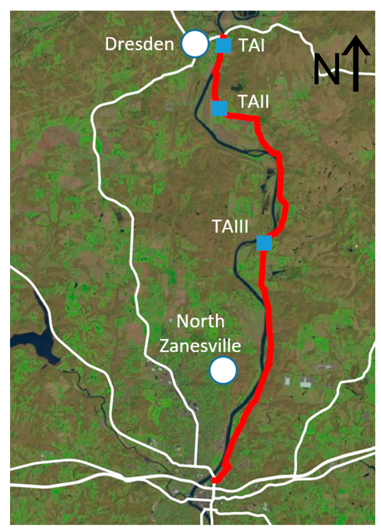
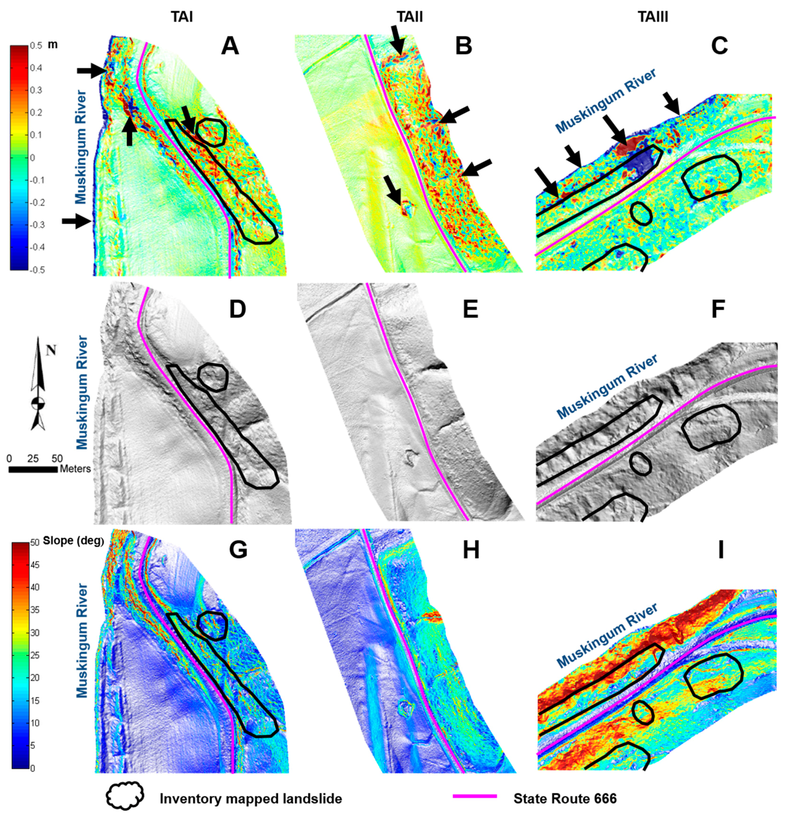
Shown in Figure 5 is the distribution of three testing areas along the study area labeled TAI, TAII and TAIII. Although, three testing areas are displayed to demonstrate our findings, our evaluation was not limited to the three and was performed for the entire study area consisting of a 23 km stretch along SR 666 composed of 80 landslides that were provided from a reference inventory. Figure 6A–C display DoD maps with areas that have undergone noticeable vertical change, where some examples are depicted by a black arrow. Figure 6D–F show bare-earth shaded relief maps made from DEMs at 0.50 m spatial resolution acquired by the 2012 LiDAR survey, where the shaded relief maps exhibit various surface features; for example, smooth and rough surface textures that may indicate landslide activity. Figure 6G–I display the slope map for each testing area. Statistically the changes observed in the study area can be modeled by a mean and standard deviation of 0.00 m and 0.18 m, respectively. This means that approximately 1 sigma of the changes are within the uncertainty level of 0.17 m, which will define approximately 68% of the detected vertical changes. Therefore, there are sufficient samples to test (~32%) and determine if the changes detected are above the uncertainty level.
The proposed DoD method detects vertical changes within the landslide inventory map (Figure 6A,C) and areas not previously mapped as landslides (Figure 6B), signifying that new developing landslides may be emerging. The statistics, for the changes observed for the testing areas displayed in Figure 6A–C, and listed in Table 2, illustrate that the small mean for TAI has a balanced mass, while TAII undergoes more accumulation or gain in mass, and TAIII undergoes more depletion in mass. In addition, the standard deviation of TAIII is significantly higher than the uncertainty level of 0.17 m, which is not the case for TAI and II, where they are similar and below the uncertainty level, respectively.
TAI (Figure 6A,D,G) demonstrates areas with high topographic variability compared to their respective neighboring regions. These rough textured areas include an inventory mapped landslide that is of particular interest as it appears to undergo accumulation (see black arrows) as shown in the DoD map. The hillshading algorithm seen in (Figure 6D–F) follows the logarithmic approach to shaded relief representation of [43].The light source was at an altitude angle of 60° and an azimuth angle of 315°. The DEM boundary on the western end of TAI is along the riverbank of the Muskingum River, therefore as bank erosion (e.g., bank scour and mass failure) occurs, mainly caused by rainfall, the mass will erode into the Muskingum River. For this reason, along the riverbank the DoD map displays depletion. In TAII, the sloped terrain undergoes higher amounts of accumulation than depletion, while flat terrain differences seem to vary as some areas undergo small amounts of accumulation and others show nearly no change. The sloped area along TAII is not within a mapped landslide from the reference inventory map and it is of interest as it may be a newly developing landslide. Interestingly, TAII displays similar dominating buildup as that in TAI, which is potentially due to accumulation. Although the slope is not particularly steep, as previously stated, slope instabilities throughout the study area range from 18–80°, in which the most frequently observed slope was 45°. TAIII is an interesting section because large amounts of landslides are clearly represented from the DoD map (Figure 6C). The vertical differences, where large (>±0.50 m) magnitudes of landslides occur, are noticeably visible and clustered together (Figure 6C). Furthermore, the northern section is along the riverbank, thus, displaying erosion. Since a landslide has occurred between the surveys, it may indicate that more frequent surveys with shorter time periods between them are necessary to detect landslides earlier and monitor their evolution. The relationships shown describe the changes observed in the DoD map, a depiction of the surface topography through relief by demonstrating the hillshade figures and slope to understand the topography of the area.

4.2. Probabilistic Change Detection

Before computing the probability map, the effect of the sample size was tested and evaluated by having varying window widths between 3 and 11 cells, resulting in the window size of 7 × 7 cells (3.5 m × 3.5 m), which provided enough samples to determine if the local neighborhood exhibited high-probability surface change. Window size varies to accommodate maximum performance of the algorithm, and therefore it is smaller than the original 9 × 9 window in the feature extraction. It was also observed that the sample size did affect the size of the high-probability clusters but did not change their location. Therefore, as the sample size increased, the cluster size decreased as expected, as the center cell evaluated has a higher correlation to cells that are closer in space, than those that are far more distant.
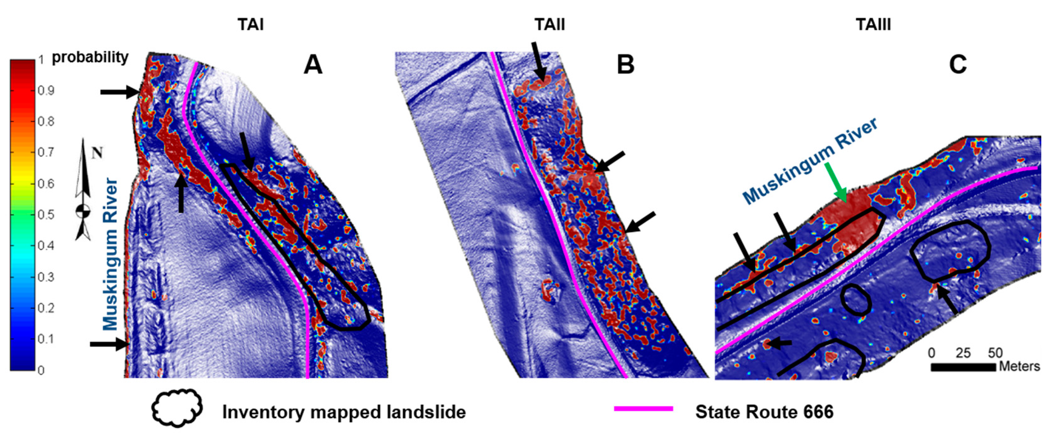
After assessing the vertical differences, the probability that each vertical difference was above the uncertainty level was evaluated using the Wilcoxon signed ranked test, which evaluates the null hypothesis (H0: Δ ≥ M). The probabilistic non-parametric signed rank test generates a probability map, shown in Figure 7A–C. The results for the non-parametric signed rank test are similar to the DoD maps shown in Figure 6A–C. It is observed for both maps that local neighborhoods having the highest amount of vertical differences also have the highest probability of the vertical change being above the uncertainty level. One limitation of the probability map, however, is that it does not differentiate between accumulation and depletion; obviously, it can easily be compared to the DoD map to determine the change type.
The results demonstrate that the computed probabilities yield a nearly binary high or low classification, which is advantageous as it simplifies the detectability of highly probable changes. Additionally, the method is shown to cluster the high probability changes, simplifying the process required to identify surface patches that may have undergone temporal changes.
The results generated from the signed rank test show that TAI, TAII and TAIII in Figure 7 exhibit surface deformations with high probability. In TAI, the changes detected coincide with the mapped landslide outlined in Figure 6D. High-probability clusters are observed along the western road edge, suggesting that these may be newly developing landslides or that the previously mapped landslide from the reference has increased in size shown in red as clusters in Figure 7A. The riverbank is also mapped with high-probability clusters, suggesting erosion in the area.
The algorithm also demonstrates highly probable changes in TAII (Figure 7B). In particular, small areas along the road bank on the eastern side of the road undergoes high-probability vertical change, which are shown with black arrows. Since the area along the slope is not mapped as a landslide in the reference inventory, the high-probability changes suggest that this may be an area prone to landslide activity, as changes are observed that could lead to a future landslide.
TAIII (see Figure 6F and Figure 7C), which is shown to have inventory mapped landslides on the northern and southern side of the road reveals highly probable changes. A landslide seems to have occurred during the span of the surveys as a large cluster of high-probability changes is depicted in Figure 7C. This figure shows (see green arrow) that the signed rank test generates a nicely outlined high-probability cluster that illustrates the shape of the potential slide, which was expected as there were high vertical changes (>±0.50 m) detected in this location. The northern side of the road demonstrates higher topographic variability in the hillshade map than the southern side of the road, which may be the reason why there is less vertical change there, and only small clusters are created that may be suppressed as noise (see black arrows). Since the northern end is along the riverbank, high-probability changes are expected along this area. Overall, this area presents a unique scenario, as the changes observed were after the potential sliding occurred and before it was repaired, which is uncommon. Since, this is an active road that is heavily used by its residents and local travelers, when a landslide occurs that directly affects the road, it is subsequently repaired by ODOT in order to keep the road open and functional. Nonetheless, the approach proposed appears to work well as it clearly identifies the highly probable temporal changes.
Although the algorithm is able to identify surface deformation along the study area, it is noted that some of the clusters may be noise or an invalid prediction by the model, rather than actual surface changes that have occurred over time. In fact, this may be the case for the emerging landslides that are considered along the western road edge (see Figure 7A) and the probable landslides described for the road bank in Figure 7B. For these reasons, additional information is required to clearly identify surface changes throughout the study area that are subject to landslides and delineate them from noise and invalid model predictions.

4.3. Landslide Surface Feature Extraction

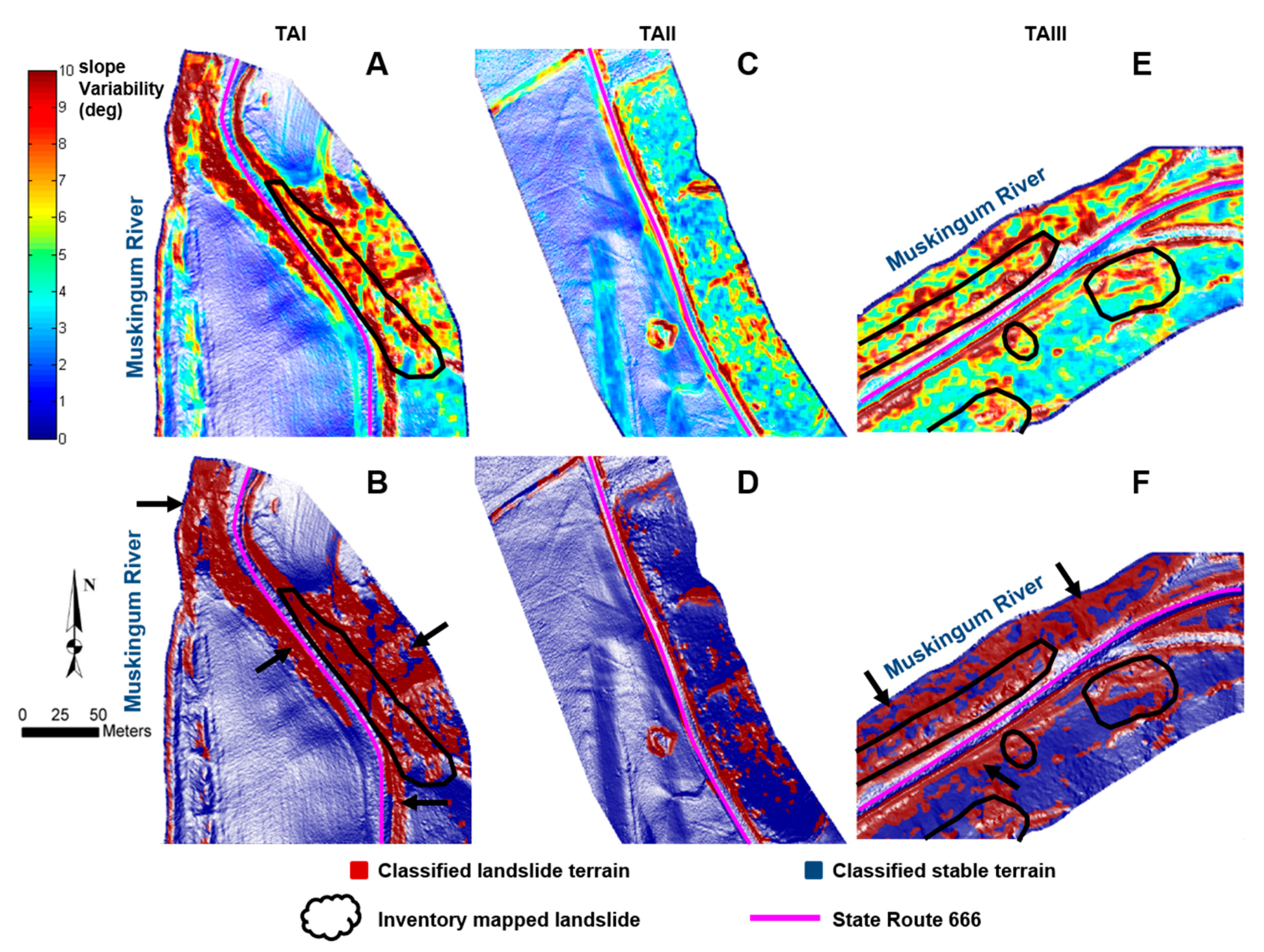
The classified locations by the proposed algorithm coincide with the areas experiencing high topographic variability for all the three testing areas and throughout the study area. The algorithm has performed properly as it was able to delineate rough and smooth topography as shown in Figure 8. The reference mapped landslides exhibit high topographic variability and the surface feature extraction algorithm is capable of identifying and classifying these surface features as landslide surface features. However, as well as the algorithm performs in identifying landslide surface features, it also overclassifies and identifies other areas that are not landslides. For example, road limits and riverbanks throughout the study area (see Figure 8), demonstrate these particular limitations related to the landslide surface feature extraction algorithm. Therefore, it is shown that areas that undergo abrupt changes in elevation, thus mimicking a scarp, will be classified as landslide surface features.

4.4. Landslide Detection

The last step of the proposed approach was to fuse the results achieved from the landslide surface feature extraction algorithm (see Section 4.3) and those subject to high probability change (see Section 4.2) to map surface deformation that has undergone landslide activity. To generate the algorithm based landslide map from the proposed method, the effect of the cluster size and probability threshold was tested. The thresholds were evaluated by having varying cluster sizes between 25 and 150 m2 and the probability threshold for the signed rank test was between 0.70 and 0.99 for cells classified as landslide prone. These ranges were selected after evaluating the minimum size of the mapped landslides provided by the reference inventory map, which was 200 m2, and aiming to have only high-probability changes, classified as having landslide surface features. After evaluating potential cluster sizes and probability thresholds, it was determined that 25 m2 and 0.90, were the most appropriate thresholds for the test dataset. The criteria selected will allow for small clusters with high probability to be mapped as significant surface changes, additionally suppressing potential noise.
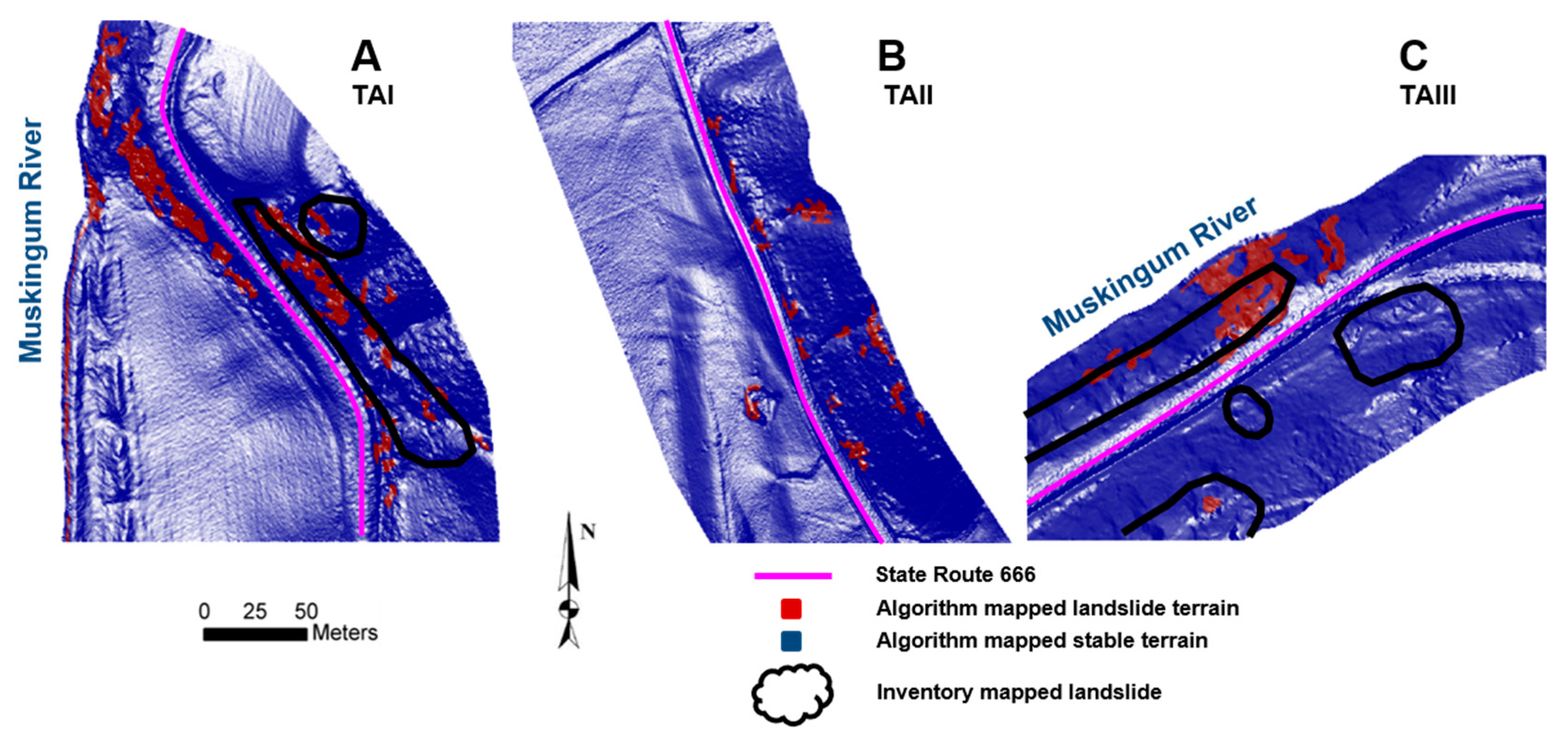
The detected areas will vary for all locations by the proposed algorithm, which reflects the difference in the topography (see Figure 9A–C). Areas that are smooth will go undetected by the proposed method, while areas that are rough may be mapped, if high probable changes are observed. Part of the areas shown in Figure 9 tend to correspond to those in Figure 6, Figure 7 and Figure 8, which are important intermediate components of the proposed approach. Additionally, some of the areas identified as landslide by the proposed algorithm tend to coincide to those mapped locations provided by the reference inventory map, verifying that the proposed model can detect landslide terrain (see Figure 9). This is not to say that the proposed approach is without any limitations. Outliers are expected to be observed as not all stable and landslide terrain will have complete coverage of surface features and changes representative of each. Therefore, it is possible to detect occurrences of stable surface features and changes in landslide terrain and conversely. These occurrences can be produced by irregularities within the terrain, noise in the data or invalid predictions by our approach. To understand and possibly improve the limitations of the proposed method further evaluation is necessary beyond the scope of this study.
The mapped landslides in TAI (Figure 9) by the proposed algorithm tend to coincide with the mapped landslides from the reference layer and those areas experiencing high topographic variability. The mapped landslides in TAII suggest that these may be new developing slides, as there are no slides provided from the reference inventory in this area. TAIII clearly maps a landslide, which displayed a high probability change and surface roughness, which suggests that more frequent surveys may be necessary to mitigate these events as the evolution of landslides may be monitored. Although, the landslide event has already occurred the proposed approach detects sliding that occurred between the LiDAR surveys that have yet to be corrected or stabilized. This suggests that the algorithm can also be used as a post-failure rapid mapping technique if pre-failure data is available.
The three testing areas illustrate different scenarios that can potentially occur, which are: (1) monitoring of existing slides; (2) identifying newly developing slides; and (3) identifying slides that occurred and were not repaired between surveys. The proposed algorithm works well in all three cases. One limitation observed is the LiDAR data spatial resolution and vertical accuracy that seems to greatly affect the algorithm’s potential performance. For sub-meter spatial resolution data, the method was able to identify 66% of the mapped landslides (53 out of a total of 80) from the inventory landslide map either experiencing landslide changes partially or fully within the reference polygons. Therefore, as long as a cluster (does not matter in size or how many clusters), is detected within an inventory mapped landslide, then the landslide will be considered as positively identified/detected. The intent of the proposed approach is not to match on a pixel-by-pixel basis every cell in the study area, which would be nearly impossible given the limitations previously described throughout the manuscript, but to flag/detect these locations to facilitate some of the work that will be required to identify them. It can be considered as if the algorithm will help flag locations that are susceptible to landslides. It is suspected that many of the detected landslides were within a close proximity of the inventory mapped landslides and could be new developing landslides. Of course, to confirm that they are not new developing landslides or landslides that were overlooked during the inventory map generation, field investigation is required to confirm the cause of the detection.
One limitation of the proposed algorithm is that it is unable to differentiate between landslide and erosion along water bodies. For the test dataset, 25% of the detected areas (clusters) by our proposed approach were along rivers, streams, and creeks, and, in addition, 13% of them were along the riverbank. These areas are known to mimic landslide surface features and undergo temporal changes through deposition and erosion. Therefore, it is obvious that they will be detected in most cases. To improve the classification algorithm, a GIS database may be used to filter out these misclassified locations. Although, the GIS database could have been included as a part of this study, it was not included as the performance of the proposed approach was to be evaluated without the inclusion of external information. Additionally, it was observed that flat terrain was mapped by the proposed approach at some locations along the study area, however, it was insignificant (~0.1% of the total classified locations). None of the flat terrain areas were mapped in Figure 9. Reference inventory mapped slides that were not detected by the proposed approach are potentially experiencing slower rates of surface change and/or display lower amounts of topographic variability. The statistics of the changes observed within the 80 inventory mapped landslides (reference) and the landslide clusters detected by the proposed algorithm that were within the inventory mapped landslides (reference) that were utilized to classify 66% (53 out of 80) of the inventory mapped slides are listed in Table 3.
The mean changes observed between the two areas analyzed (inventory mapped areas and algorithm mapped w/in inventory slides over the entire study area) are similar and close to a balanced deposition and erosion of mass. However, the variation is higher for the mapped areas by the algorithm within the landslide inventory locations (see Table 3). This may be due to the algorithm’s ability to classify only local neighborhoods susceptible to changes greater than the uncertainty level of 0.17 m with a high degree of probability; consequently, having high surface deformation in either depletion or accumulation. Meanwhile, the inventory mapped slides consider all changes, even those with a low degree of probability of the changes being real, e.g., those experiencing no change or below the uncertainty level causing the variation to decrease. The variation of the changes detected within the entire inventory mapped landslides is similar to that of the uncertainty level. The distribution shown in Figure 10A illustrates a normal distribution for the changes detected in the entire inventory of mapped landslides, while those detected by the algorithm within the inventory of mapped landslides (Figure 10B) do not reveal a normal distribution and appear as a bimodal Gaussian distribution. The peak shown in Figure 10A is around 0 m, while the peaks shown in Figure 10B are above the propagated uncertainty level of ±0.17 m. The changes detected, in theory, are expected to indicate a loss in material at higher elevations of the slope and a gain at the lower elevations due to erosion and deposition. However, this is not the case for all changes detected because they vary in each location and there is no clear pattern observed between them in the DoD maps (see Figure 6). The only location displaying this pattern is shown in Figure 6C where the major landslide has occurred.
It is noted that the areas frequently mapped by the proposed algorithm coincide with those consisting of landslide geomorphologic characteristics and high probable change. These areas are comprised of saturated material, vegetation and slopes that on average are 45°, which are higher than areas that do not suffer slope instabilities. In addition, the soils found in these locations are known to cause slope instabilities that are typically activated by ground movement, slope alteration, saturation, and low internal strength. These events are generally triggered by intense rainfall, roadway improvements (the initial construction of the roadway itself), and are more likely to occur at locations where the roadway is near the river. For example, colluvial soils are one of the most predominate soil types found within the study area. Slope instability associated with ground movement of the colluvial mass can be triggered by any minor amount of slope alteration (re-working of the slope or addition of ground or surface water). Several areas along SR 666 were noted for being a severe hazard to roadway construction due to low strength, susceptibility to frost action, and high erosion potential. General signs of moist to wet soils within the study area are found in hydrophytic plants such as willow trees, sedges, lilies, cat tails, ferns, and duck grass [31], which increase the possibility of slope instability. Additionally, thick lush vegetation, muddy areas or areas of ponded water during dry periods can indicate wet soils.

5. Discussion and Conclusions

The proliferation of remote sensing data offers new opportunities for affordable measurement, including, the exploitation of large 3D data sets such as point clouds or surface for landslide detection. In particular, airborne LiDAR has been continuously used for its ability to penetrate the canopy, cover large swaths of terrain and provide the accuracy necessary to map surface models accurately. Methods of change detection, especially DoD maps, are of interest, as the availability and affordability of airborne LiDAR data continues to improve [37]. For these reasons, we proposed an algorithm that fuses probabilistic change detection and feature extraction to identify small landslide features from multi-temporal airborne LiDAR-derived DEMs. Prior studies have focused on the evolution of a single small landslide (e.g., [26,27]). Conversely, we focus on multiple over large swaths of terrain, having various surface changes on a wide variety of surface topography and complexities. In addition, we assess the detection of small failures in terms of spatial extent, which most studies overlook.
For the study data, it was observed that the propagated uncertainties significantly impacted the detectability of vertical changes; ±0.17 m. The proposed method can only be as accurate as the surface models used for landslide detection. Since the method employs many independent processes, the incorporation of more advanced techniques may result in further improvements. Vertical changes below the propagated uncertainties are neglected, in our case they are large changes since our focus are small deformations, however, as airborne LiDAR technology improves the uncertainty will decrease and minor changes will be detected.
The proposed approach, based on a probabilistic, non-parametric signed rank test evaluates high-probability temporal changes exhibited in landslide-prone terrain. Geomorphic changes are unlikely to be uniformly distributed, especially when failures are small and local neighborhoods are considered, for this reason a non-parametric evaluation was performed. However, since our uncertainties are large (±0.17 m) small changes are difficult to identify and are neglected. One of the benefits of the algorithm is its ability to omit outliers that are caused by errors rather than change. Note a limitation of its dependency on the propagated uncertainties, which are driven by the surface model accuracy. If uncertainties can be reduced, however, the algorithm will identify more subtle changes. Nonetheless, sub-meter change detection can be achieved if the registration between multi-temporal data sets is properly aligned and bare-earth surface models are used cautiously, especially in vegetated areas.
The characterization of surface topography is essential to detect surface changes of landslide activity using multi-temporal surface models. In the investigation it was observed that areas depicting higher degrees of topographic variability than local neighboring terrain were more likely to be mapped as a landslide, which corresponds to the idea that the surfaces of landslides are not as smooth and continuous as neighboring un-failed terrain, described and proved in [2,6,17,37]. Important factors to consider when developing a detection algorithm are the impacts caused by saturated material, vegetation, slopes and the underlying soil. These factors help interpret and analyze the occurrence of landslide events that were detected by the proposed method. In the proposed algorithm, surface features found in landslide morphology are used to filter changes that do not display landslide activity. This step in the approach will help filter the results by solely detecting temporal changes that exhibit landslide features.
Clearly, the main limiting factor to monitor the spatial and temporal processes of landslides is the availability of high-quality DEM data [12]. The spatial resolution of the airborne LiDAR data acquired at approximately 50 cm is evidently not the spacing needed to map the relevant surface features found in small landslides. Therefore, the airborne LiDAR data was limited for extracting small features triggered by the small landslides found in our study, consequently, the resolution impacted the performance of the proposed landslide detection algorithm.
Although our LiDAR data at approximately 50 cm was limited in spatial resolution, the performance of the algorithm was satisfactory. To test and evaluate the algorithm, a thorough analysis was performed to quantify the surface formations of new landslides, areas susceptible to landslides, and landslide scars compared to the landslide inventory map of the area. The results of this study indicate that the monitoring of existing and identification of newly developing landslides are feasible, where 66% of the mapped landslides (53 out of a total of 80) in the study area were detected as having landslide changes when compared to the inventory landslide map. Furthermore, the results of the algorithm on our data set are comparable in performance to [44] who detected approximately 70% of landslides in their study using change detection and image fusion. Additionally, most studies overlook the surface component in their studies (e.g., [26,27]), which is a vital characteristic on which our proposed technique is based.
As airborne LiDAR continues to advance, the improvements will provide higher spatial resolutions, terrain coverage and improved accuracy necessary to map surface models with higher precision, thus, allowing for improved change detection. Similarly, as uncertainties are reduced with advanced measurements, DoD methods can be improved [12], allowing for increased confidence in landslide mapping results. For these reasons, the optimal spatial resolution for landslide detection is determined by considering the accuracy, quantity of data, and the scale of the landslide surface features [17].

Acknowledgments

The authors wish to acknowledge the support of Kirk Beach from the Office of Geotechnical Engineering of the Ohio Department of Transportation. Also, the authors wish to acknowledge Tien Wu for his insight and feedback throughout this study.

Author Contributions

Omar E. Mora, M. Gabriela Lenzano, Charles K. Toth, and Dorota A. Grejner-Brzezinska conceived and designed the experiments; Omar E. Mora performed the experiments; Omar E. Mora, M. Gabriela Lenzano, Charles K. Toth, Dorota A. Grejner-Brzezinska, and Jessica V. Fayne analyzed the experimental results; Omar E. Mora, M. Gabriela Lenzano, and Jessica V. Fayne contributed figures/materials; Omar E. Mora, M. Gabriela Lenzano, and Jessica V. Fayne wrote the paper.

Conflicts of Interest

The authors declare no conflict of interest.

References

  1. Guzzetti, F.; Carrara, A.; Cardinali, M.; Reichenbach, P. Landslide hazard evaluation: A review of current techniques and their application in a multi-scale study, Central Italy. Geomorphology 1999, 31, 181–216. [Google Scholar] [CrossRef]
  2. Booth, A.M.; Roering, J.J.; Perron, J.T. Automated landslide mapping using spectral analysis and high-resolution topographic data: Puget Sound lowlands, Washington, and Portland Hills, Oregon. Geomorphology 2009, 109, 132–147. [Google Scholar] [CrossRef]
  3. Martha, T.R.; Kerle, N.; van Westen, C.J.; Jetten, V.; Kumar, K.V. Segment optimization and data-driven thresholding for knowledge-based landslide detection by object-based image analysis. IEEE Trans. Geosci. Remote Sens. 2011, 49, 4928–4943. [Google Scholar] [CrossRef]
  4. Ballabio, C.; Sterlacchini, S. Support vector machines for landslide susceptibility mapping: The Staffora River Basin case study, Italy. Math. Geosci. 2012, 44, 47–70. [Google Scholar] [CrossRef]
  5. Tien Bui, D.; Pradhan, B.; Lofman, O.; Revhaug, I. Landslide susceptibility assessment in Vietnam using Support vector machines, Decision tree and Naïve Bayes models. Math. Probl. Eng. 2012, 2012, 974638. [Google Scholar] [CrossRef]
  6. McKean, J.; Roering, J. Objective landslide detection and surface morphology mapping using high-resolution airborne laser altimetry. Geomorphology 2004, 57, 331–351. [Google Scholar] [CrossRef]
  7. Galli, M.; Ardizzone, F.; Cardinali, M.; Guzzetti, F.; Reichenbach, P. Comparing landslide inventory maps. Geomorphology 2008, 94, 268–289. [Google Scholar] [CrossRef]
  8. Wang, L.-J.; Sawada, K.; Moriguchi, S. Landslide-susceptibility analysis using light detection and ranging-derived digital elevation models and logistic regression models: A case study in Mizunami City, Japan. J. Appl. Remote Sens. 2013, 7, 073561. [Google Scholar] [CrossRef]
  9. Lane, S.N.; Richards, K.S.; Chandler, J.H. Developments in monitoring and modelling small-scale river bed topography. Earth Surface Processes Landf. 1994, 19, 349–368. [Google Scholar] [CrossRef]
  10. Wheaton, J.M.; Brasington, J.; Darby, S.E.; Merz, J.; Pasternack, G.B.; Sear, D.; Vericat, D. Linking geomorphic changes to salmonid habitat at a scale relevant to fish. River Res. Appl. 2010, 26, 469–486. [Google Scholar] [CrossRef]
  11. Wheaton, J.M.; Brasington, J.; Darby, S.E.; Sear, D.A. Accounting for uncertainty in DEMs from repeat topographic surveys: Improved sediment budgets. Earth Surf. Processes Landf. 2010, 35, 136–156. [Google Scholar] [CrossRef]
  12. DeLong, S.B.; Prentice, C.S.; Hilley, G.E.; Ebert, Y. Multitemporal ALSM change detection, sediment delivery, and process mapping at an active earthflow. Earth Surf. Processes Landf. 2012, 37, 262–272. [Google Scholar] [CrossRef]
  13. Kelsey, H.M. Earthflows in Franciscan mélange, Van Duzen River basin, California. Geology 1978, 6, 361–364. [Google Scholar] [CrossRef]
  14. Baum, R.L.; Messerich, J.; Fleming, R.W. Surface deformation as a guide to kinematics and three-dimensional shape of slow-moving, clay-rich landslides, Honolulu, Hawaii. Environ. Eng. Geosci. 1998, 4, 283–306. [Google Scholar] [CrossRef]
  15. Malet, J.-P.; Maquaire, O.; Calais, E. The use of Global Positioning System techniques for the continuous monitoring of landslides: Application to the Super-Sauze earthflow (Alpes-de-Haute-Provence, France). Geomorphology 2002, 43, 33–54. [Google Scholar] [CrossRef]
  16. Chadwick, J.; Dorsch, S.; Glenn, N.; Thackray, G.; Shilling, K. Application of multi-temporal high-resolution imagery and GPS in a study of the motion of a canyon rim landslide. ISPRS J. Photogramm. Remote Sens. 2005, 59, 212–221. [Google Scholar] [CrossRef]
  17. Glenn, N.F.; Streutker, D.R.; Chadwick, D.J.; Thackray, G.D.; Dorsch, S.J. Analysis of LiDAR-derived topographic information for characterizing and differentiating landslide morphology and activity. Geomorphology 2006, 73, 131–148. [Google Scholar] [CrossRef]
  18. Mackey, B.H.; Roering, J.J.; McKean, J.A. Long-term kinematics and sediment flux of an active earthflow, Eel River, California. Geology 2009, 37, 803–806. [Google Scholar] [CrossRef]
  19. Coe, J.A.; McKenna, J.P.; Godt, J.W.; Baum, R.L. Basal-topographic control of stationary ponds on a continuously moving landslide. Earth Surf. Processes Landf. 2009, 34, 264–279. [Google Scholar] [CrossRef]
  20. Mackey, B.H.; Roering, J.J. Sediment yield, spatial characteristics, and the long-term evolution of active earthflows determined from airborne LiDAR and historical aerial photographs, Eel River, California. Geol. Soc. Am. Bull. 2011, 123, 1560–1576. [Google Scholar] [CrossRef]
  21. Cheng, K.S.; Wei, C.; Chang, S.C. Locating landslides using multi-temporal satellite images. Adv. Space Res. 2004, 33, 296–301. [Google Scholar] [CrossRef]
  22. Lu, P.; Stumpf, A.; Kerle, N.; Casagli, N. Object-oriented change detection for landslide rapid mapping. IEEE Geosci. Remote Sens. Lett. 2011, 8, 701–705. [Google Scholar] [CrossRef]
  23. Daehne, A.; Corsini, A. Kinematics of active earthflows revealed by digital image correlation and DEM subtraction techniques applied to multi-temporal LiDAR data. Earth Surf. Processes Landf. 2013, 38, 640–654. [Google Scholar] [CrossRef]
  24. Ventura, G.; Vilardo, G.; Terranova, C.; Sessa, E.B. Tracking and evolution of complex active landslides by multi-temporal airborne LiDAR data: The Montaguto landslide (Southern Italy). Remote Sens. Environ. 2011, 115, 3237–3248. [Google Scholar] [CrossRef]
  25. Tseng, C.M.; Lin, C.W.; Stark, C.P.; Liu, J.K.; Fei, L.Y.; Hsieh, Y.C. Application of a multi-temporal. LiDAR-derived, digital terrain model in a landslide-volume estimation. Earth Surf. Processes Landf. 2013, 38, 1587–1601. [Google Scholar] [CrossRef]
  26. Caris, J.P.T.; van Asch, T.W. Geophysical, geotechnical and hydrological investigations of a small landslide in the French Alps. Eng. Geol. 1991, 31, 249–276. [Google Scholar] [CrossRef]
  27. Garel, E.; Marc, V.; Ruy, S.; Cognard-Plancq, A.L.; Klotz, S.; Emblanch, C.; Simler, R. Large scale rainfall simulation to investigate infiltration processes in a small landslide under dry initial conditions: The Draix hillslope experiment. Hydrol. Process. 2012, 26, 2171–2186. [Google Scholar] [CrossRef]
  28. James, L.A.; Hodgson, M.E.; Ghoshal, S.; Latiolais, M.M. Geomorphic change detection using historic maps and DEM differencing: The temporal dimension of geospatial analysis. Geomorphology 2012, 137, 181–198. [Google Scholar] [CrossRef]
  29. Wehr, A.; Lohr, U. Airborne laser scanning—An introduction and overview. ISPRS J. Photogramm. Remote Sens. 1999, 54, 68–82. [Google Scholar] [CrossRef]
  30. Shan, J.; Toth, C.K. (Eds.) Topographic Laser Ranging and Scanning: Principles and Processing; CRC Press: Boca Raton, FL, USA, 2008. [Google Scholar]
  31. Ohio Department of Transportation Office of Geotechnical Engineering. Report of Findings, Geohazard Inventory and Evaluation, MUS-666-0.00. Available online: www.dot.state.oh.us/Divisions/Planning/SPR/Research/reportsandplans/Reports/2015/Geotechnical/134609_ES.pdf (accessed on 20 November 2017).
  32. Isenburg, M. LAStools—Efficient Tools for LiDAR Processing. Version 111216. Available online: http://lastools.org (accessed on 20 November 2017).
  33. Mora, O.E.; Lenzano, M.G.; Toth, C.K.; Grejner-Brzezinska, D.A. Analyzing the Effects of Spatial Resolution for Small Landslide Susceptibility and Hazard Mapping. Int. Arch. Photogramm. Remote Sens. Spat. Inf. Sci. 2014, XL-1, 293–300. [Google Scholar] [CrossRef]
  34. Brasington, J.; Langham, J.; Rumsby, B. Methodological sensitivity of morphometric estimates of coarse fluvial sediment transport. Geomorphology 2003, 53, 299–316. [Google Scholar] [CrossRef]
  35. Wilcoxon, F. Individual comparisons by ranking methods. Biometrics 1945, 1, 80–83. [Google Scholar] [CrossRef]
  36. Hollander, M.; Wolfe, D.A.; Chicken, E. Nonparametric Statistical Methods; John Wiley & Sons: New York, NY, USA, 2013; Volume 751. [Google Scholar]
  37. Mora, O.E.; Liu, J.K.; Lenzano, M.G.; Toth, C.K.; Grejner-Brzezinska, D.A. Small Landslide Susceptibility and Hazard Assessment Based on Airborne Lidar Data. Photogramm. Eng. Remote Sens. 2015, 81, 239–247. [Google Scholar] [CrossRef]
  38. Vapnik, V. The Nature of Statistical Learning; Springer: New York, NY, USA, 2000. [Google Scholar]
  39. Samui, P. Slope stability analysis: A support vector machine approach. Environ. Geol. 2008, 56, 255–267. [Google Scholar] [CrossRef]
  40. Yao, X.; Tham, L.G.; Dai, F.C. Landslide susceptibility mapping based on support vector machine: A case study on natural slopes of Hong Kong, China. Geomorphology 2008, 101, 572–582. [Google Scholar] [CrossRef]
  41. Marjanović, M.; Kovačević, M.; Bajat, B.; Voženílek, V. Landslide susceptibility assessment using SVM machine learning algorithm. Eng. Geol. 2011, 123, 225–234. [Google Scholar] [CrossRef]
  42. Micheletti, N.; Foresti, L.; Kanevski, M.; Pedrazzini, A.; Jaboyedoff, M. Landslide Susceptibility Mapping Using Adaptive Support Vector Machines and Feature Selection. Master’s Thesis, University of Lausanne, Lausanne, Switzerland, 2011; 99p. [Google Scholar]
  43. Katzil, Y.; Doytsher, Y. A logarithmic and sub-pixel approach to shaded relief representation. Comput. Geosci. 2003, 29, 1137–1142. [Google Scholar] [CrossRef]
  44. Nichol, J.; Wong, M.S. Satellite remote sensing for detailed landslide inventories using change detection and image fusion. Int. J. Remote Sens. 2005, 26, 1913–1926. [Google Scholar] [CrossRef]
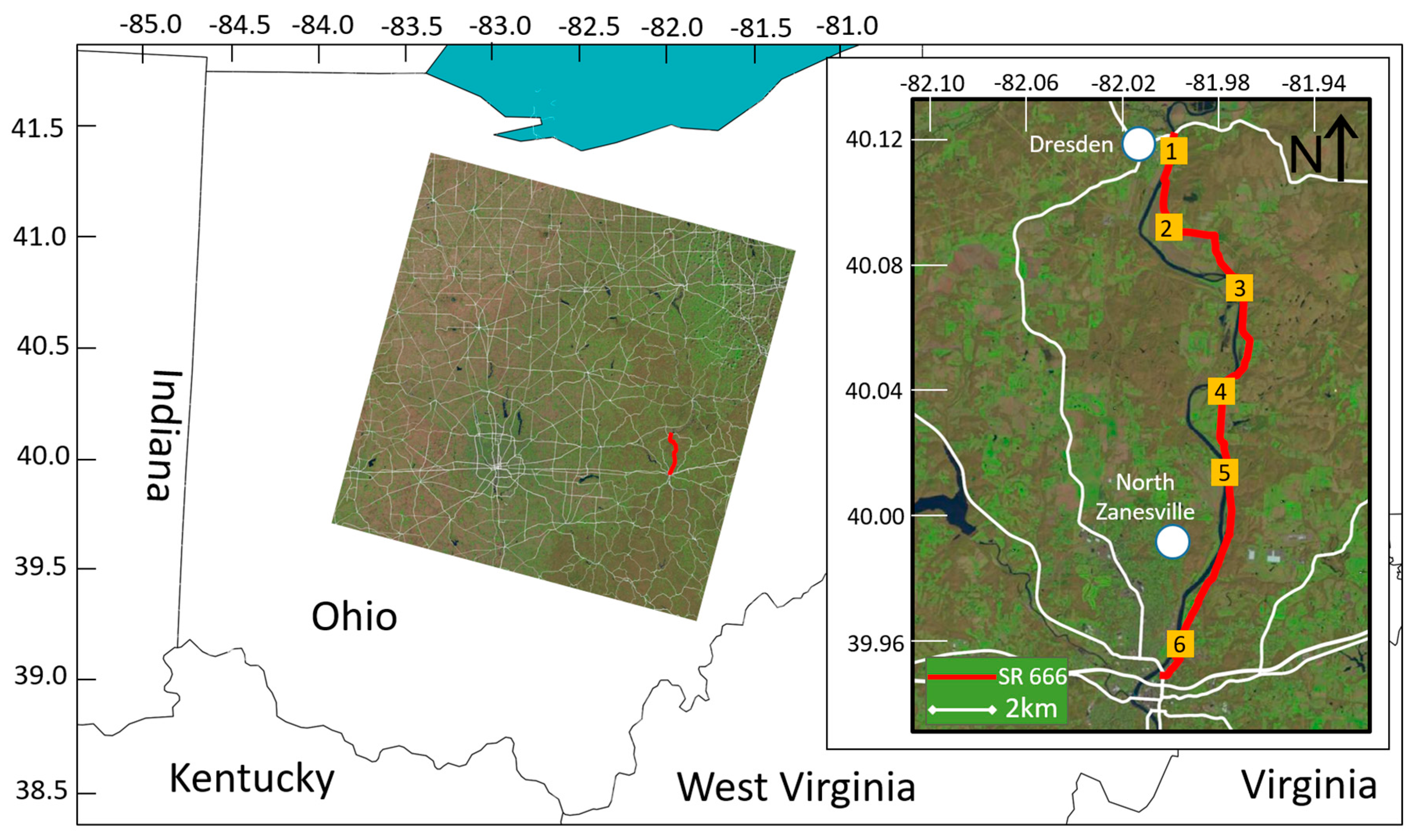
Figure 1. The study area along the transportation corridor SR-666, north of Zanesville, OH, is in close proximity of the Muskingum River. The orange squares indicate the location of the six independent segments along the study area that were used for the LiDAR accuracy assessment.
Geosciences 08 00023 g001
Figure 2. Examples of rotational slides affecting the embankment, near SR-666 Mile Marker (MM) 7.3 (A) and MM 1.47 (B). The landslide upper sections/scarps are outlined in red in both examples. Figures modified from [31].
Geosciences 08 00023 g002
Figure 3. Workflow to detect and map landslide temporal changes.
Geosciences 08 00023 g003
Figure 4. Vertical error distribution between the interpolated DEM and LiDAR point cloud for the six segments (see Figure 1) evaluated for the 2008 and 2012 datasets of SR 666.
Geosciences 08 00023 g004
Figure 5. Distribution of Testing Areas (TA) -I, -II, and -III along SR 666 shown by blue squares.
Geosciences 08 00023 g005
Figure 6. DoD maps (top) are shown in (AC). Hillshade maps (middle) are shown in (DF) for the 2012 DEM. Slope maps (bottom) are shown in (GI) for the 2012 DEM. Examples of areas experiencing vertical changes are depicted by black arrows.
Geosciences 08 00023 g006
Figure 7. Illustrated in (AC) are the probabilities (signed rank test) for TAI, TAII and TAIII, respectively, for a local neighborhood of 7 × 7 cells and M = 0.17 m. Examples of areas undergoing high probable change are depicted by arrows.
Geosciences 08 00023 g007
Figure 8. Illustrated in (A,C,E) are the surface roughness maps and in (B,D,F) are the classified maps for TAI, TAII and TAIII, respectively. Examples of overclassified areas are depicted by black arrows.
Geosciences 08 00023 g008
Figure 9. Mapped slides with underlying DEM for TAI (A), TAII (B) and TAIII (C).
Geosciences 08 00023 g009
Figure 10. Distribution of vertical changes observed between the 2012 and 2008 DEMs. (A): vertical changes observed within the inventory mapped landslides (reference), and (B): vertical changes mapped by the proposed approach within the inventory mapped landslides.
Geosciences 08 00023 g010
Table 1. Accuracy assessment of the differences between the interpolated DEM and LiDAR point cloud of the six segments shown in Figure 4 for the 2008 and 2012 DEMs.
Segment #No. PtsMean (m)STD (m)Min (m)Max (m)RMSE (m)
200820122008201220082012200820122008201220082012
1424154480.050.020.120.120.000.000.820.760.120.12
2318137100.010.010.140.070.000.000.840.550.140.08
3758910,0570.060.020.090.090.000.000.580.550.110.09
446106597−0.030.010.080.080.000.000.320.340.080.08
545645460−0.020.020.130.130.000.000.720.710.130.13
6486671250.040.010.080.090.000.000.671.290.090.09
Total29,05138,3970.020.010.110.100.000.000.841.290.110.10
Table 2. Statistics of the DoD maps (vertical changes) for TAI, TAII, and TAIII shown in Figure 6 demonstrate the loss and gain of mass within the selected regions.
Testing AreasMean (m)Median (m)STD (m)
TAI0.010.010.18
TAII0.070.050.12
TAIII−0.030.000.29
Table 3. Statistics of vertical changes detected; (A): vertical changes detected within the inventory mapped landslides (reference), and (B): vertical changes detected by the algorithm within the inventory mapped landslides.
Changes Detected (Units: m)MeanMedianSTD
Inventory Mapped Slides (A)0.010.020.17
Algorithm Mapped w/in Inventory Slides (B)0.020.180.48