Spatiotemporal Characteristics and Trends of Climate Extremes in and Around the Yunnan Reach of the Nujiang River Basin

Abstract

Daily observations from 14 stations and ERA5 reanalysis were used to examine temperature, precipitation, and wind extremes in and around the Yunnan reach of the Nujiang River Basin during 1991–2020. Twelve station indices, two reanalysis-derived wind indices, and circulation diagnostics describe their spatial, seasonal, and interannual variability. The regional annual maximum of daily maximum temperature (TXx) and annual minimum of daily minimum temperature (TNn) increased by 0.50 and 0.55 °C per decade, respectively. Warm-night and warm-day frequencies increased by 3.98 and 3.00 percentage points (pp) per decade, whereas cold-night and cold-day frequencies decreased by 2.67 and 2.87 pp per decade. Recorded wet-day precipitation had a fitted trend of −69.27 mm per decade (Newey–West 95% confidence interval: −110.03 to −28.51 mm per decade; p = 0.002), with considerable interannual variability (R² = 0.135). Climatological wet-day precipitation ranged from 847.46 mm at Yunxian to 2016.39 mm at Longling over the study period. Using identical station thresholds and matched valid days, ERA5 warm-day, cold-night, and heavy-precipitation frequencies differed from observations by −5.89, +7.14, and +0.40 pp, respectively. ERA5 annual maximum hourly 10 m wind speed showed no significant regional trend (+0.01 m s⁻¹ per decade; p = 0.791). Seasonal circulation and humidity fields provide context for the observed annual cycle of temperature and precipitation extremes. Overall, the station network shows a shift towards warmer temperature extremes and strong spatial contrasts in precipitation; ERA5 captures shared annual frequency variations while yielding different mean frequencies and event dates, supporting separate evaluation of temporal covariability and local event occurrence.

1. Introduction

Climate change is altering the occurrence and magnitude of weather and climate extremes [1]. The IPCC Sixth Assessment Report documents widespread increases in hot extremes and decreases in cold extremes since the 1950s, together with increases in heavy precipitation in many regions [2]. Indices derived from daily temperature and precipitation records provide a consistent way to summarize such changes [3]. Their interpretation requires explicit thresholds, reference periods, and temporal aggregation, particularly when observations and gridded reanalyses are compared. Land-surface processes also affect extremes: modeling studies assess irrigation effects on temperature [4], while urban rainfall research examines the influence of urbanization [5].

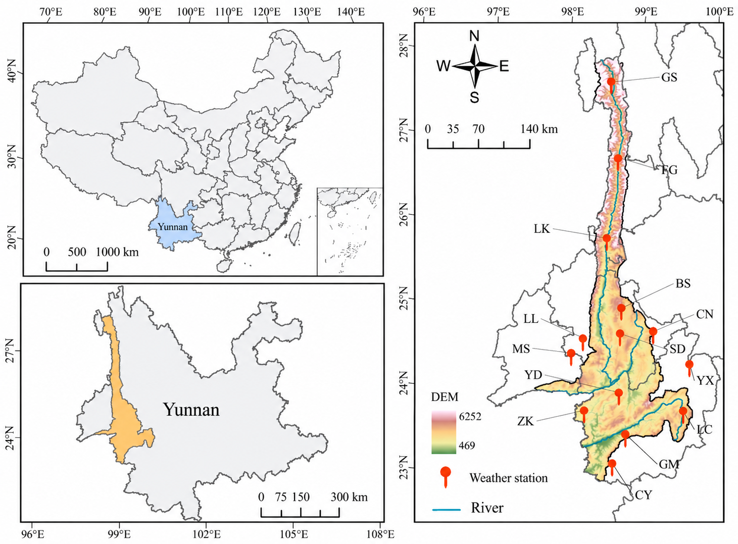
Studies across China show substantial changes in temperature extremes, with regional differences in their magnitude [6,7]. Evidence from the Tibetan Plateau also indicates elevation-dependent responses [8,9,10]. Precipitation studies have quantified greenhouse-gas contributions across Chinese climate zones [11], locally opposite warming responses in the 2023 Beijing–Tianjin–Hebei rainfall event [12], and the dynamics of sequential precipitation–heatwave events [13]. The Yunnan reach of the Nujiang River Basin (Figure 1) occupies a transition between mountain and valley environments influenced by the Asian monsoon circulation. Previous regional work has described its climate and long-term changes [14] and identified multiple summer water-vapor transport pathways [15]. These findings motivate a station-based assessment that separates the spatial distribution of extreme index values from their temporal trends.

Figure 1. Location of the Nujiang–Salween River Basin, the Yunnan reach examined in this study and the 14 meteorological stations. The orange-shaded area in the overview maps indicates the Yunnan reach of the Nujiang River Basin. Colours in the right-hand map show terrain elevation (m). The red markers indicate the meteorological stations, and the blue lines indicate rivers. Station abbreviations and elevations are listed in Table 1.

Figure 1. Location of the Nujiang–Salween River Basin, the Yunnan reach examined in this study and the 14 meteorological stations. The orange-shaded area in the overview maps indicates the Yunnan reach of the Nujiang River Basin. Colours in the right-hand map show terrain elevation (m). The red markers indicate the meteorological stations, and the blue lines indicate rivers. Station abbreviations and elevations are listed in Table 1.

Table 1. Meteorological stations used in this study.

ID	Station	Code	Elevation (m)
56533	Gongshan	GS	1583.3
56641	Fugong	FG	1176.7
56643	Liuku	LK	949.8
56748	Baoshan	BS	1668.4
56839	Zhenkang	ZK	1053.8
56842	Shidian	SD	1487.4
56849	Yongde	YD	1606.2
56951	Lincang	LC	1636.1
56843	Changning	CN	1666.9
56844	Mangshi	MS	913.8
56841	Longling	LL	1630.6
56944	Cangyuan	CY	1278.3
56946	Gengma	GM	1144.1
56854	Yunxian	YX	1108.6

Table 1. Meteorological stations used in this study.

ID	Station	Code	Elevation (m)
56533	Gongshan	GS	1583.3
56641	Fugong	FG	1176.7
56643	Liuku	LK	949.8
56748	Baoshan	BS	1668.4
56839	Zhenkang	ZK	1053.8
56842	Shidian	SD	1487.4
56849	Yongde	YD	1606.2
56951	Lincang	LC	1636.1
56843	Changning	CN	1666.9
56844	Mangshi	MS	913.8
56841	Longling	LL	1630.6
56944	Cangyuan	CY	1278.3
56946	Gengma	GM	1144.1
56854	Yunxian	YX	1108.6

Asian climate variability also reflects connections between tropical Pacific conditions and circulation outside the tropics. Tian et al. [16] discuss spatially contrasting East Asian climate changes and ENSO links on palaeoclimatic timescales, while Serykh et al. [17] examine the connections between ENSO and extratropical teleconnections. These studies provide a wider context for considering monsoon and Pacific indices; the relationships during 1991–2020 are assessed here directly from the corresponding annual records.

The present study addresses three questions: how do temperature and precipitation extremes vary among 14 meteorological stations within and around the Yunnan reach and through time; what additional information is provided by ERA5 wind extremes and seasonal circulation fields; and how do extreme-event frequencies derived from ERA5 differ from station records under common thresholds? The analysis combines station indices, hourly reanalysis calculations, monthly circulation diagnostics, and explicit tests of circulation–index associations. The geographical focus is the Yunnan reach and its surrounding station network.

2. Materials and Methods

2.1. Overview of the Study Area

The Nujiang–Salween River crosses the southeastern Tibetan Plateau and the Hengduan Mountains. This study examines its Yunnan reach in southwestern China and a network of 14 stations within and around that reach (Figure 1; Table 1). The supplied terrain raster, clipped to the Yunnan basin boundary, gives elevations of approximately 469–6252 m above sea level. The station elevations range from 913.8 to 1668.4 m. Narrow valleys and adjacent mountain ranges accompany substantial local climatic contrasts within the regional monsoon setting [14,15]. Research on the wider Nujiang–Salween basin has documented glacier retreat [18] and projected snow-related runoff changes [19]; ecological planning in Nujiang Prefecture also considers the sensitivity of its alpine-valley terrain [20].

2.2. Data Sources and Quality Control

Daily maximum, minimum, and mean temperature and daily precipitation were assembled for the 14 stations from 1 January 1991 to 31 December 2020. Table 1 summarizes the 14 meteorological stations used in this study, including their station IDs, abbreviations, and elevations. Regional series are equal-weight means across the station network; they describe the 14-station observational footprint within and around the Yunnan reach, rather than an area-weighted mean for the entire Nujiang River Basin. A wet day is defined here as a day with recorded precipitation greater than 1 mm.

Quality control checked date coverage, duplicate records, negative numerical precipitation, and consistency between daily maximum and minimum temperatures. Each station contains 10,958 dated rows, giving 153,412 station-days in total. The analyses use 153,411 valid daily maximum-temperature values, 153,411 valid daily minimum-temperature values, 153,408 valid daily mean-temperature values, and 138,066 numerical daily precipitation values. One maximum/minimum temperature record at Lincang is non-numeric; non-numeric precipitation flags are excluded from numerical calculations without zero filling. Availability is reported by station in Table S1. Percentile frequencies use valid temperature days as their denominator, and precipitation totals and counts summarize the numerically recorded values. All observation–ERA5 frequency comparisons use exactly the same valid dates in both datasets.

ERA5 [21] was used at two temporal resolutions. Hourly single-level fields supplied 2 m temperature, total precipitation, 10 m zonal and meridional wind, and surface pressure on the 0.25° grid distributed through the Earth Engine catalog (ECMWF/ERA5/HOURLY). Monthly pressure-level fields supplied wind components, geopotential, relative humidity, and specific humidity for 1991–2020. Circulation maps use 200, 500, and 700 hPa; vertical wind profiles use levels from 700 to 200 hPa, and moisture-flux-divergence sections use eight levels from 1000 to 300 hPa. The hourly data support event calculations, and the monthly fields describe the circulation background. ERA5 data are available through the Copernicus Climate Data Store (https://cds.climate.copernicus.eu/).

The South Asian Summer Monsoon Index (SASMI) follows the dynamically normalized seasonality definition of Li and Zeng [22], which measures the seasonal reversal of 850 hPa winds over South Asia (5–22.5° N, 35–97.5° E). We use the provider’s June–September (JJAS) seasonal series. The East Asian index is specifically the monsoon vector projection index, EASMI-MVPI [23]: it measures the south-minus-north contrast in summer wind-vector projection anomalies along the climatological monsoon direction. Its supplied June–August (JJA) series is used.

SOI characterizes the standardized Tahiti–Darwin sea-level pressure contrast, while Niño 3.4 represents sea-surface temperature anomalies over 5° S–5° N, 170–120° W. Multi-index ENSO studies also examine the related but distinct temporal behavior of these indicators [24]. PDO represents the leading pattern of North Pacific sea-surface temperature variability after removal of the global-mean signal [25]. Monthly SOI, Niño 3.4, and PDO series were obtained from NOAA PSL and averaged over JJA. The five circulation series were restricted to 1991–2020; their definitions, provider addresses, and seasonal windows are compiled in Table S2. The JJA SASMI is also evaluated as a seasonal sensitivity check (Table S4).

2.3. Methods

2.3.1. Temperature and Precipitation Indices

The 12 station indices comprise four annual temperature extremes, four percentile-based temperature frequencies, and four precipitation indices (

Table 2. Definitions of the station indices. Percentile thresholds use the fixed, pooled 1991–2020 baseline specified in Section 2.3.1.

Index	Definition	Unit
TXx	Annual maximum value of daily maximum temperature	°C
TNx	Annual maximum value of daily minimum temperature	°C
TXn	Annual minimum value of daily maximum temperature	°C
TNn	Annual minimum value of daily minimum temperature	°C
TN10p	Percentage of days with daily minimum temperature below the 10th percentile	%
TX10p	Percentage of days with daily maximum temperature below the 10th percentile	%
TN90p	Percentage of days with daily minimum temperature above the 90th percentile	%
TX90p	Percentage of days with daily maximum temperature above the 90th percentile	%
PRCPTOT	Sum of recorded precipitation on days with daily precipitation > 1 mm	mm
SDII	Ratio of total precipitation on wet days (>1 mm) to the number of wet days	mm d−1
R10mm	Annual count of recorded days with daily precipitation ≥ 10 mm	d
R20mm	Annual count of recorded days with daily precipitation ≥ 20 mm	d

), drawing on the climate-index framework of Zhang et al. [3]. Temperature thresholds are the station-specific 10th and 90th percentiles of all valid daily values pooled over 1991–2020. They are fixed through time and applied to annual and monthly records. Thus, the percentile indices in this study use a pooled annual baseline, rather than calendar-day percentile thresholds. This definition retains the seasonal concentration of threshold exceedances. Strict inequalities define temperature exceedances; precipitation-day counts include values equal to 10 or 20 mm.

2.3.2. Linear Trends and Statistical Associations

An ordinary least-squares model was fitted to each unsmoothed annual series: y(t) = a + bt + ε(t). Here, y(t) is the annual index value, t is the calendar year, a is the intercept, b is the annual slope, and ε(t) is the residual. The slope is b = Σ[(t − $\overline{\mathrm{t}}$)(y − $\overline{\mathrm{y}}$)]/Σ(t − $\overline{\mathrm{t}}$)². The symbols $\overline{\mathrm{t}}$ and $\overline{\mathrm{y}}$ denote the means of year and annual index value, respectively. Trends are reported as 10b, in units per decade. Frequency trends are expressed in percentage points (pp) per decade, i.e., absolute changes in a frequency expressed as a percentage. Conventional two-sided OLS slope tests and R² accompany all regional trends in Table 3; p < 0.05 denotes nominal significance. Station-level values and slopes are provided in Table S3. Serial-correlation diagnostics and alternative trend tests are given in Tables S10–S12.

Table 3. Linear trends of all 12 regional station indices, 1991–2020. Tests use the 30 unsmoothed annual values. p denotes the conventional two-sided OLS slope-test probability. Serial-correlation-robust tests are reported in Tables S10 and S11. p and R² are reported to six decimal places; p-values below 10⁻⁶ use scientific notation. pp = percentage points.

Index	Trend per Decade	Unit	p (OLS)	R2
TXx	+0.50	°C	0.001979	0.293709
TNx	+0.39	°C	0.000003	0.549961
TXn	+0.16	°C	0.597089	0.010107
TNn	+0.55	°C	0.000252	0.385408
TN10p	−2.67	pp	3.04 × 10−9	0.720834
TX10p	−2.87	pp	0.000432	0.362433
TN90p	+3.98	pp	2.44 × 10−10	0.766361
TX90p	+3.00	pp	0.000014	0.495840
PRCPTOT	−69.27	mm	0.045491	0.135334
SDII	−0.08	mm day−1	0.597189	0.010102
R10mm	−2.21	days	0.069369	0.112974
R20mm	−1.18	days	0.068812	0.113401

Table 3. Linear trends of all 12 regional station indices, 1991–2020. Tests use the 30 unsmoothed annual values. p denotes the conventional two-sided OLS slope-test probability. Serial-correlation-robust tests are reported in Tables S10 and S11. p and R² are reported to six decimal places; p-values below 10⁻⁶ use scientific notation. pp = percentage points.

Index	Trend per Decade	Unit	p (OLS)	R2
TXx	+0.50	°C	0.001979	0.293709
TNx	+0.39	°C	0.000003	0.549961
TXn	+0.16	°C	0.597089	0.010107
TNn	+0.55	°C	0.000252	0.385408
TN10p	−2.67	pp	3.04 × 10−9	0.720834
TX10p	−2.87	pp	0.000432	0.362433
TN90p	+3.98	pp	2.44 × 10−10	0.766361
TX90p	+3.00	pp	0.000014	0.495840
PRCPTOT	−69.27	mm	0.045491	0.135334
SDII	−0.08	mm day−1	0.597189	0.010102
R10mm	−2.21	days	0.069369	0.112974
R20mm	−1.18	days	0.068812	0.113401

Temporal autocorrelation was assessed from the lag-one autocorrelation of the raw annual series and OLS residuals, together with Ljung–Box tests on the residuals [26]. The main diagnostic jointly tests residual lags one to three; one- and five-lag tests are also reported. As a uniform sensitivity analysis, OLS slopes were tested using Newey–West heteroscedasticity- and autocorrelation-consistent standard errors [27], with Bartlett weights and a primary maximum lag of three years. The covariance estimate uses the finite-sample factor n/(n − 2), and two-sided p-values and 95% confidence intervals use a Student t reference with n − 2 = 28 degrees of freedom. Maximum lags of one to five years were evaluated for every series using the same settings. This approach changes the estimated uncertainty while retaining the original slope, annual values, and event definitions. Tables S10–S12 report all regional and station-level results, including cases where the significance classification changes. For the three-lag diagnostics, Benjamini–Hochberg q-values [28] are calculated separately across the 16 regional and 168 station–index series.

Pearson correlations compare each of the five seasonal circulation indices with the 30 annual regional values from the same calendar years of each station index. The analysis reports r and two-sided p-values for the raw series (28 degrees of freedom) and for residuals after removal of a linear time trend. The latter are partial correlations controlling for time, tested with 27 degrees of freedom. Benjamini–Hochberg-adjusted q-values [28] are calculated separately for the 60 raw and 60 detrended tests. Here, q denotes the p-value adjusted for multiple testing; q < 0.05 is the criterion for a 5% false discovery rate within each test family. This reporting separates associations that include long-term covariation from associations in interannual residual variability (Table S4).

Each correlation pairs a summer circulation state with the annual climate index from the same calendar year. This aggregation asks whether years with different summer monsoon or Pacific conditions also differ in their annual extreme-event summary. It retains the annual indices used in the trend analysis and the provider-defined monsoon seasons. Summer is relevant to the observed July maxima in precipitation and warm-night occurrence, although warm days peak in May and cold events peak in January (Section 3.2.1). Annual indices also include events outside JJA/JJAS; these correlations therefore combine summer and non-summer contributions and do not isolate a summer-specific event response. No lead–lag prediction or causal effect is estimated.

2.3.3. Smoothing and Seasonal Summaries

A centered three-year moving average, M(t) = [y(t − 1) + y(t) + y(t + 1)]/3, is displayed for 1992–2019 to show shorter-term variations around the annual series. Trend estimation and significance tests use all 30 unsmoothed annual values. Cumulative event-day counts are calculated for each calendar month over 1991–2020; dividing these counts by 30 gives the climatological mean monthly counts reported in the text.Station–year heatmaps use anomalies divided by each station’s sample standard deviation (Figures S1–S3).

2.3.4. Wind Extremes and Pressure-Level Wind Climatology

Hourly 10 m wind speed is calculated as W = (u₁₀² + v₁₀²)^1/2 at the ERA5 grid cell nearest each reference station, where u₁₀ and v₁₀ are the eastward and northward 10 m wind components (m s⁻¹), respectively. The daily maximum is the largest hourly speed in the 24 h reporting window. WSx is the annual maximum of these daily maxima. W95d is the number of days whose daily maximum exceeds the grid cell’s fixed 95th percentile over 1991–2020. The threshold is calculated separately for each co-located grid cell; regional WSx and W95d are equal-weight means across the 14 locations. WSx is expressed in m s⁻¹, and W95d in days per year.

For the pressure-level background, the magnitude ($\overline{\mathrm{u}}$² + $\overline{\mathrm{v}}$²)^1/2 is first calculated from the monthly mean wind components at each co-located grid cell, then averaged across locations. Here, $\overline{\mathrm{u}}$ and $\overline{\mathrm{v}}$ are the monthly mean eastward and northward wind components (m s⁻¹), respectively. Monthly climatologies, seasonal vertical profiles, and annual anomalies are derived from this series. DJF, MAM, JJA, and SON denote December–February, March–May, June–August, and September–November. A pressure level is excluded if it lies beneath the ERA5 model terrain. For the profiles, values are excluded when the pressure level exceeds the surface pressure; for the circulation maps, values are excluded when pressure-level geopotential is less than or equal to model-surface geopotential. These excluded map cells are shown by gray hatching. All 14 locations remain available at 700 hPa in the monthly profiles.

2.3.5. Matched Observation–ERA5 Extreme-Event Comparison

At each station, ERA5 was sampled from the nearest 0.25° grid cell without lapse-rate adjustment or bias correction. Daily ERA5 maximum and minimum temperatures are the extrema of the 24 hourly 2 m values ending at 12:00 UTC (20:00 China Standard Time) on the nominal date. Daily precipitation is the sum of the 24 one-hour accumulations ending at the same time, converted from meters to millimeters. This reporting window matches the station precipitation field PRE_Time_2020; the same window is used consistently for the hourly temperature and wind summaries.

Three examples are evaluated: warm days above station TX’s 90th-percentile threshold, cold nights below station TN’s 10th-percentile threshold, and heavy-precipitation days with at least 20 mm. The same observed temperature threshold is applied to both datasets. For dataset D at station s in year y, frequency is f(D,s,y) = 100 × N(D,s,y)/n(s,y), where N is the number of days satisfying the event criterion, and n is the number of shared valid dates. The difference is Δf = f(ERA5) − f(station), in pp (absolute percentage-point differences). Means are calculated across the 30 years and 14 stations with equal weights. This common-threshold design compares the frequency of equivalent temperature or precipitation conditions.

Annual event frequencies were calculated on the shared valid dates for each variable at each station, then averaged with equal weights across the 14 stations for each year. Pearson correlations were calculated between the resulting 1991–2020 regional series. Each series was also fitted separately against year by ordinary least squares, and the correlation between the two residual series was calculated to describe detrended interannual covariability. Detrending was applied only to the correlation analysis; event classifications and the frequencies in the curves and tables retain the original paired daily values and thresholds. The temperature examples compare common fixed observation-based thresholds pooled over 1991–2020, as defined above.

Daily correspondence was evaluated by station and date. H denotes days identified by both datasets, M denotes days identified only by observations, F denotes days identified only by ERA5, and C denotes days identified by neither dataset; H + M + F + C equals the number of shared valid station-days. The probability of detection (POD), false alarm ratio (FAR), and critical success index (CSI) are H/(H + M), F/(H + F), and H/(H + M + F), respectively. Metrics were calculated for each station and from counts pooled across all stations. A zero denominator was recorded as NA. The variable-specific valid-date masks, fixed observed thresholds, and daily reporting window described above were retained (Tables S8 and S9).

2.3.6. Monthly Circulation and Dry/Wet Examples

Climatological March, July, and October maps summarize winds, geopotential height (geopotential divided by 9.80665 m s⁻²), and relative humidity at 200, 500, and 700 hPa. July anomalies are calculated relative to the 1991–2020 July mean. The dry example, 2009, has the lowest regional annual recorded PRCPTOT and below-average July precipitation; the wet example, 2016, has positive annual and July anomalies. Mapped anomalies and co-located regional averages describe the circulation accompanying these two examples.

Moisture-flux-divergence sections describe the monthly circulation background along 98° E from 22° to 28° N. For March, July, and October, the specific-humidity and wind fields were each averaged over the corresponding months in 1991–2020. Horizontal moisture-flux components were formed as $\overline{\mathrm{q}}\overline{\mathrm{u}}$/g and $\overline{\mathrm{q}}\overline{\mathrm{v}}$/g, where $\overline{\mathrm{q}}$ is the monthly mean specific humidity (kg kg⁻¹), $\overline{\mathrm{u}}$ and $\overline{\mathrm{v}}$ are monthly mean eastward and northward winds (m s⁻¹), and g = 9.81 m s⁻². Horizontal derivatives were evaluated on the longitude–latitude grid and interpolated to 100 points along the section at 1000, 925, 850, 700, 600, 500, 400, and 300 hPa. Values are expressed in g cm⁻² hPa⁻¹ s⁻¹.

3. Results

3.1. Spatiotemporal Variability of Extreme Climate Indices

Regional OLS trend magnitudes, conventional significance levels, and variance explained are presented together in Table 3; serial-correlation sensitivity results are given in Tables S10–S12. Spatial contrasts are described in Section 3.1.1, the corresponding annual evolution in Section 3.1.2, and ERA5 wind extremes in Section 3.1.3.

3.1.1. Spatial Differentiation

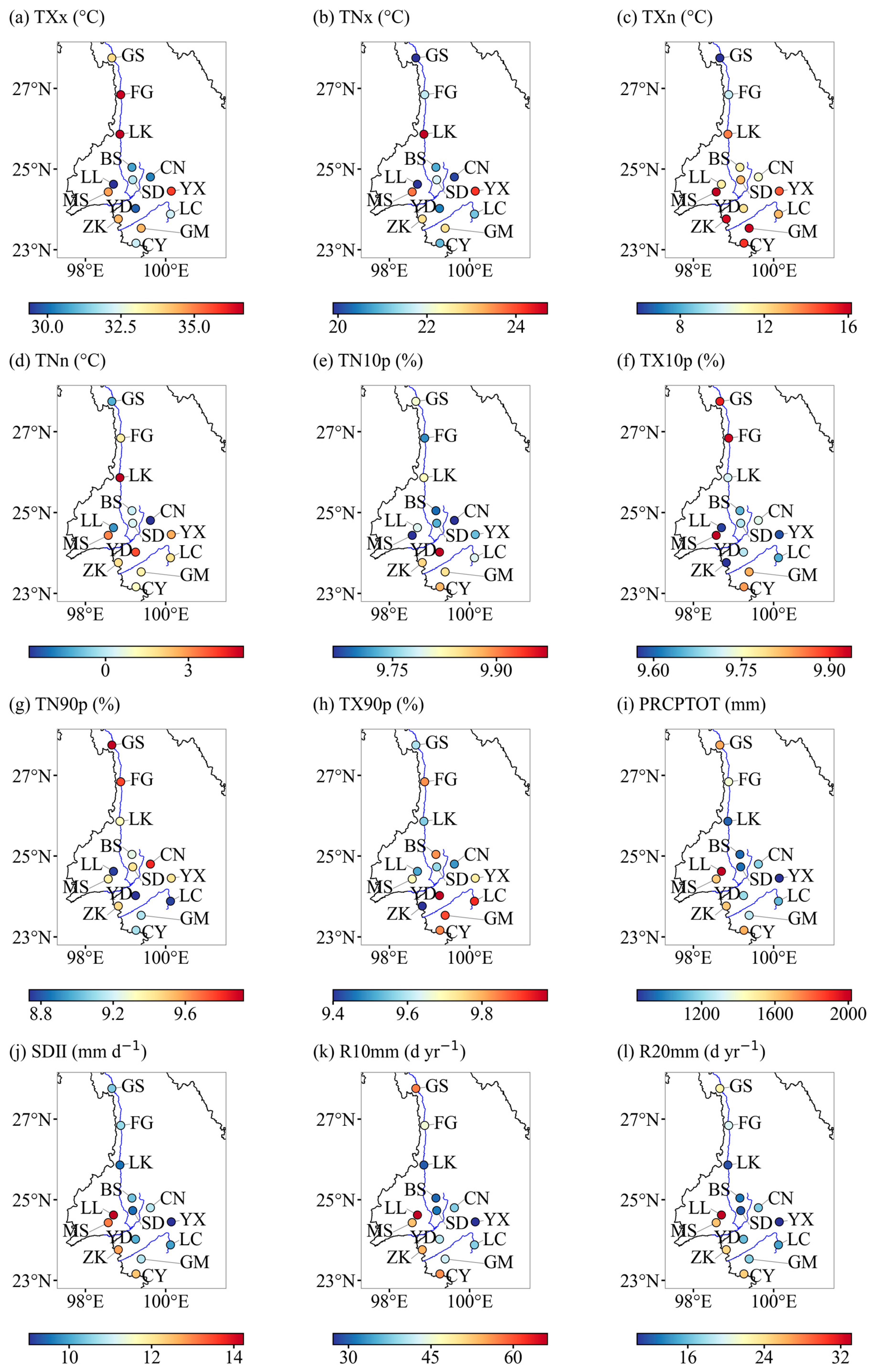
The annual temperature extremes differ substantially among stations (Figure 2; Table S3). Climatological TXx ranges from 29.37 °C at Longling to 36.67 °C at Liuku, while TNx ranges from 19.89 °C at Gongshan to 24.70 °C at Liuku. TXn ranges from 5.94 °C at Gongshan to 16.14 °C at Mangshi, and TNn ranges from −2.76 °C at Changning to 4.98 °C at Liuku. These contrasts describe the thermal environments represented by the individual stations.

The climatological percentile frequencies span 9.66–9.97% for cold nights, 9.57–9.94% for cold days, 8.73–9.92% for warm nights, and 9.40–9.98% for warm days (Figure 2e–h). Warm-night frequencies increase at all stations, with slopes of 2.12–5.37 pp per decade, while warm-day slopes range from 1.16 to 4.29 pp per decade. Cold-night and cold-day slopes are negative at all 14 stations (−6.60 to −0.24 and −3.93 to −1.86 pp per decade, respectively; Table S3).

Precipitation indices have pronounced spatial contrasts (Figure 2; Table S3). Longling has the largest climatologically recorded PRCPTOT (2016.39 mm), SDII (14.23 mm day⁻¹), R10mm (66.20 days), and R20mm (33.10 days). The corresponding minima occur at Yunxian: 847.46 mm, 9.02 mm day⁻¹, 27.17 days, and 10.70 days. Thus, the maximum-to-minimum contrast exceeds twofold for total wet-day precipitation and threefold for R20mm. The station comparison quantifies the spatial pattern within the sampled mountain–valley network.

3.1.2. Annual Variability and Trends

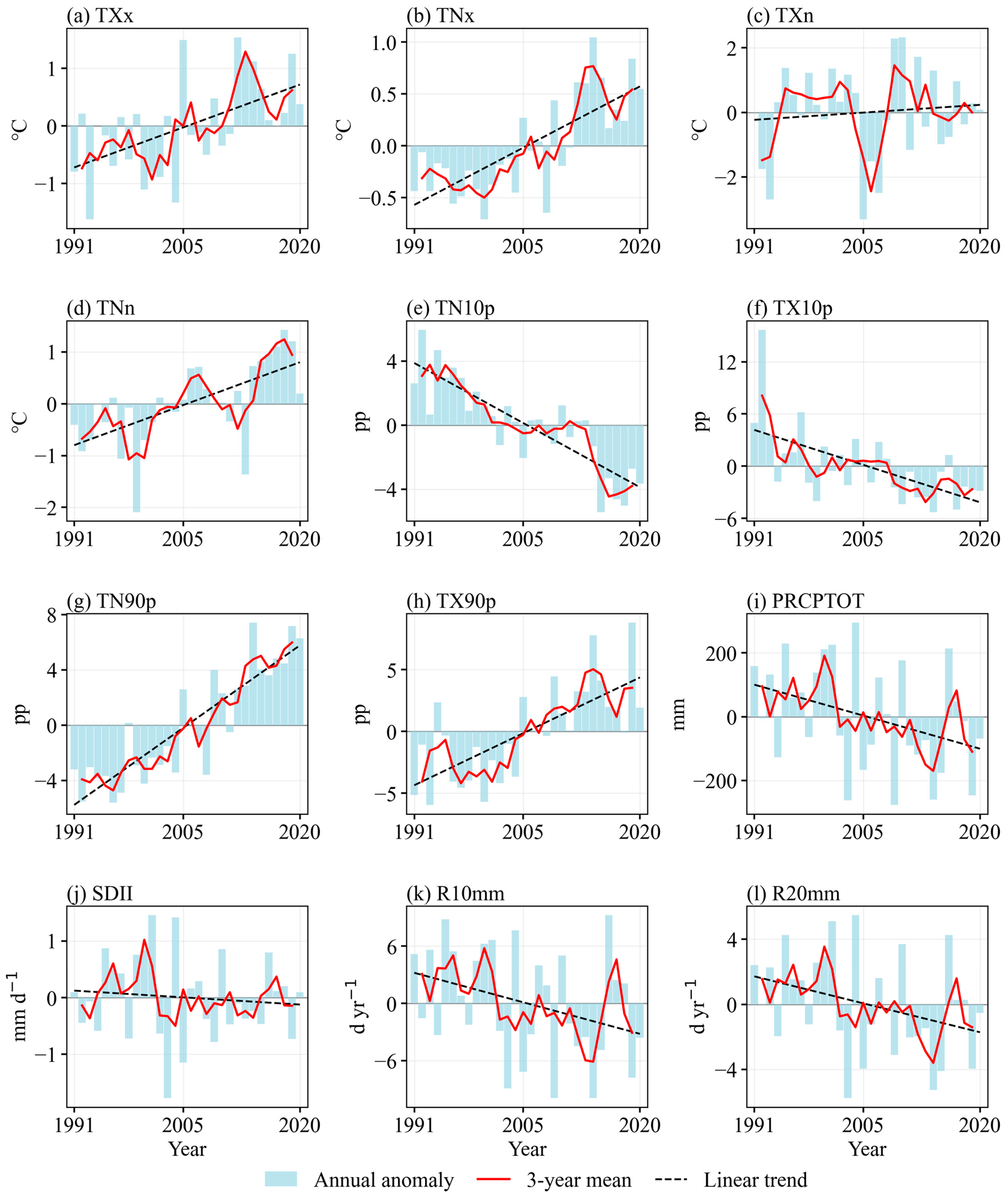
Under conventional OLS tests, the regional temperature series show increasing warm extremes and decreasing cold-event frequencies (Figure 3; Table 3). TXx, TNx, and TNn increase by 0.50, 0.39, and 0.55 °C per decade, respectively (p = 0.002, p < 0.001, and p < 0.001). TXn increases by 0.16 °C per decade, but its slope is not significant (p = 0.597089). Warm-night and warm-day frequencies increase by 3.98 and 3.00 pp per decade; cold-night and cold-day frequencies decrease by 2.67 and 2.87 pp per decade (all p < 0.001). The regional annual mean temperature increases by 0.38 °C per decade (p < 0.001; R² = 0.625).

Removing the linear trend substantially reduces the positive lag-one autocorrelation of several temperature series: for example, TN90p changes from 0.696 to −0.091. None of the 12 regional extreme-index residual series rejects the three-lag Ljung–Box diagnostic at the nominal 0.05 level (Table S10). Mean temperature gives p = 0.0258, although no regional diagnostic remains significant after adjustment across the 16 series. At the station level, 17 of 168 diagnostics have p < 0.05, and three retain q < 0.05 (Table S12). The increasing TXx, TNx, TNn, TN90p, and TX90p trends and decreasing TN10p and TX10p trends remain significant under all five Newey–West lag choices (all p < 0.005); TXn remains non-significant. Mean-temperature warming also remains significant (Table S11).

The annual ranges give the magnitude of variability around these trends. Regional TXx varies from 31.41 °C in 1993 to 34.57 °C in 2012. TN90p ranges from 3.69% in 1996 to 16.71% in 2014, and TX90p from 3.76% in 1993 to 18.49% in 2019. TXn reaches its minimum of 9.43 °C in 2005. Figures S1–S3 display the year-to-year anomalies at every station, and Figure 3 shows the corresponding network-mean annual series.

Recorded PRCPTOT ranges from 1036.99 mm in 2009 to 1608.39 mm in 2004, with a 1991–2020 mean of 1313.48 mm (Figure 3). Its OLS slope is −69.27 mm per decade (p = 0.045), with R² = 0.135. The Newey–West test with a maximum lag of three years gives p = 0.0017 and a 95% confidence interval of −110.03 to −28.51 mm per decade. The decline remains significant across maximum lags of one to five years (p = 0.00025–0.01191; Tables S10 and S11). R10mm and R20mm decline by 2.21 and 1.18 days per decade, respectively, with conventional OLS p-values of 0.069369 and 0.068812. Their Newey–West p-values are 0.0172 and 0.0034, respectively, and remain below 0.05 for all five lag choices. Their significance classification therefore differs between the two approaches. SDII has a slope of −0.08 mm day⁻¹ per decade (OLS p = 0.597189; Newey–West p = 0.352). Accordingly, the precipitation results combine a modest fitted decline in recorded wet-day totals with substantial annual variability.

3.1.3. ERA5 Near-Surface Wind Extremes

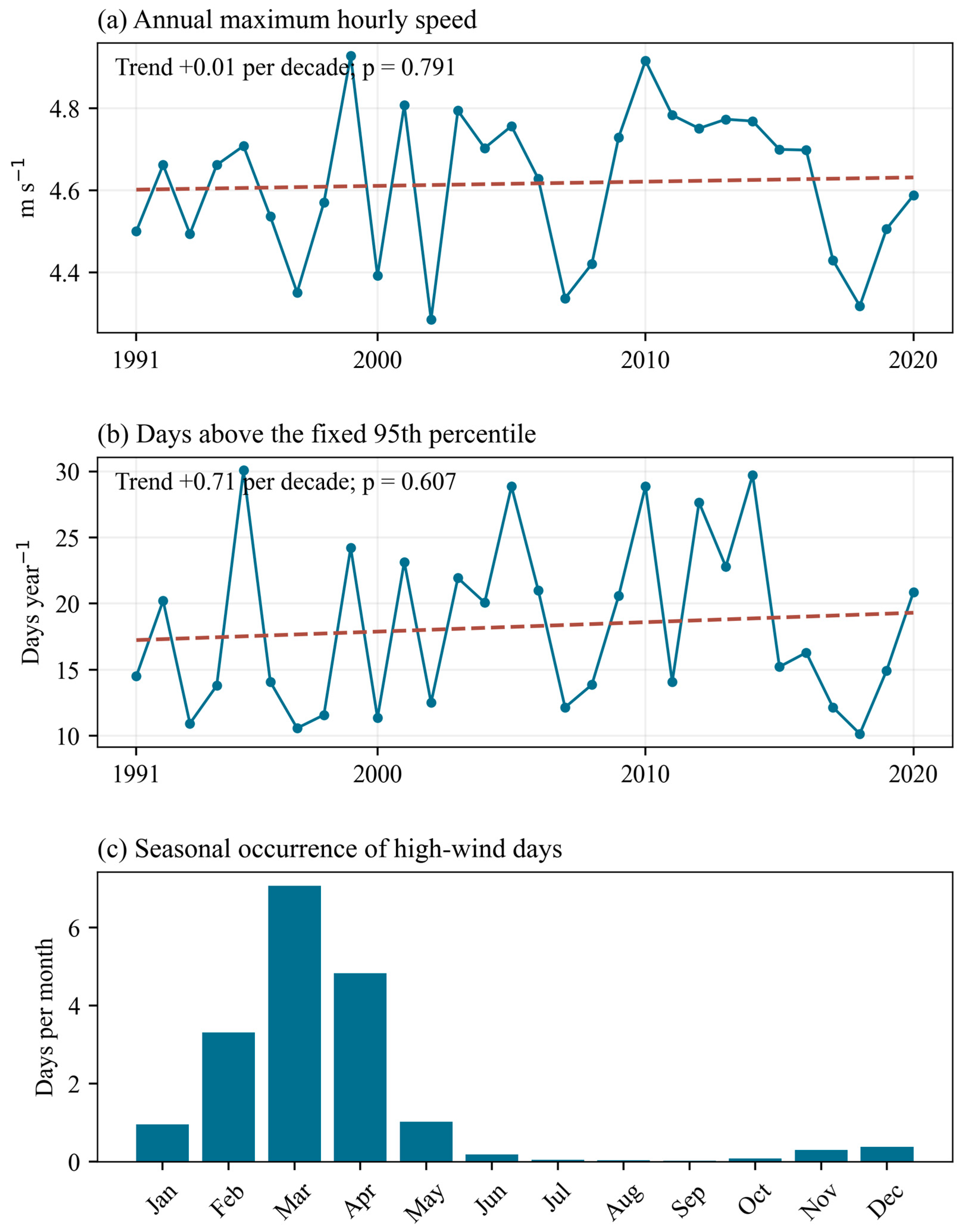
The regional mean of the annual maximum hourly 10 m wind speed is 4.62 m s⁻¹, with annual values ranging from 4.29 to 4.93 m s⁻¹ (Figure 4a). Its fitted trend is +0.01 m s⁻¹ per decade (p = 0.791). Grid-cell 95th-percentile thresholds for the daily maximum hourly wind speed range from 1.95 to 4.48 m s⁻¹ (Table S5). Regional W95d varies from 10.14 to 30.07 days per year, with a mean of 18.27 days and a trend of +0.71 days per decade (p = 0.607; Figure 4b). The approximately 5% full-period occurrence follows the percentile definition; its annual and monthly distribution shows how exceedances are distributed within that period (Figure 4c). Neither wind index has a significant linear trend over 1991–2020 under the conventional OLS or Newey–West tests (the latter give p = 0.796 for WSx and p = 0.599 for W95d; Tables S10 and S11).

3.2. Seasonal Variability and Circulation Background

3.2.1. Seasonal Characteristics

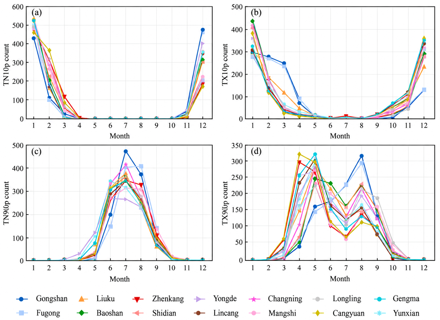
The fixed annual-baseline thresholds produce contrasting seasonal distributions of temperature events (Figure 5). The regional mean monthly count, obtained by dividing the plotted 30-year totals by 30 and averaging across stations, peaks in January at 16.69 days for cold nights and 11.90 days for cold days. Warm nights peak in July at 11.73 days, whereas warm days peak in May at 8.58 days, followed by 6.33 days in August.

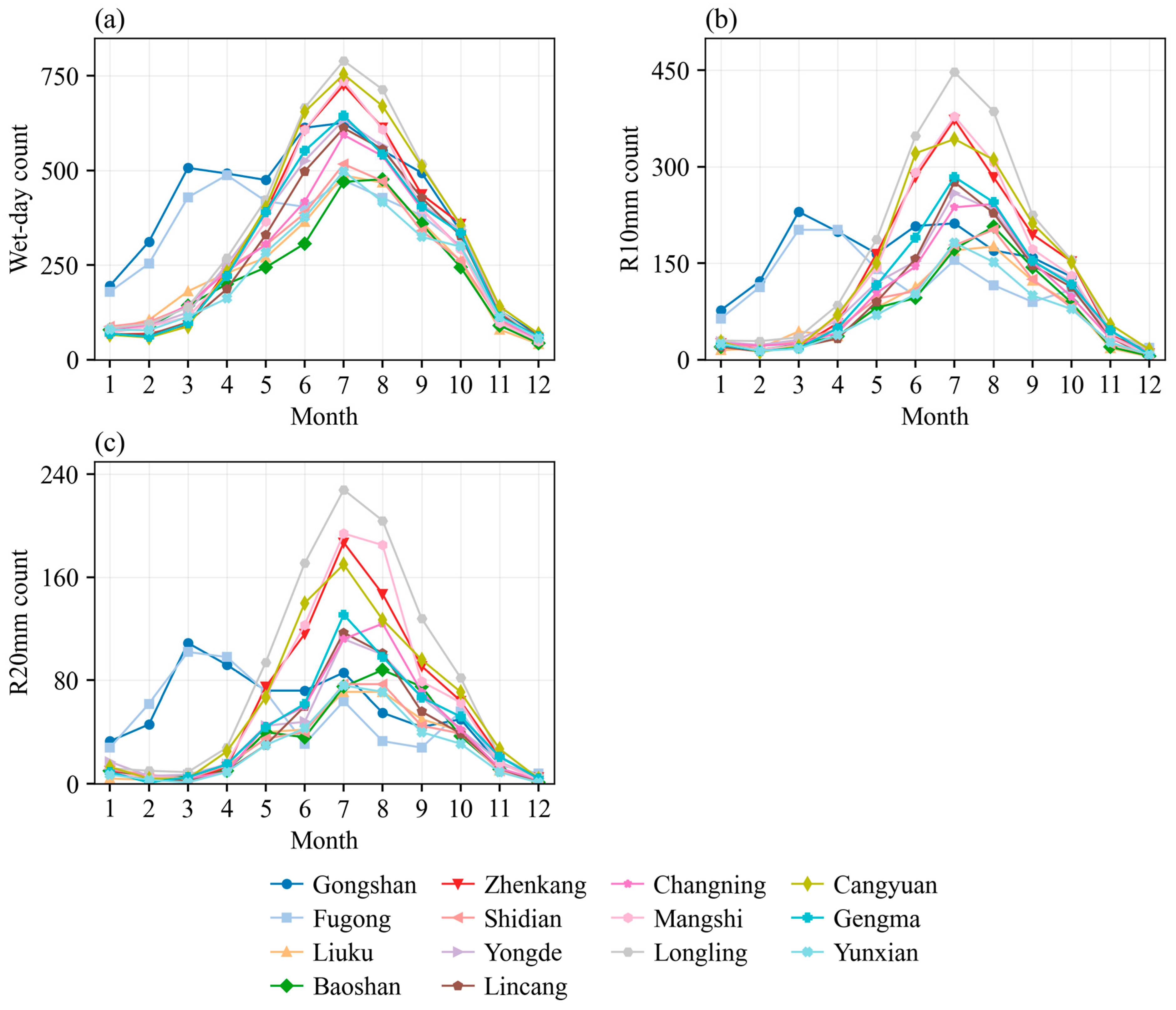
Precipitation occurrence is concentrated in the summer months (Figure 6). Regional mean monthly wet-day, R10mm, and R20mm counts peak in July at 20.39, 8.73, and 4.05 days, respectively; the corresponding December counts are 1.83, 0.35, and 0.12. The station curves show local differences in the timing and strength of the monthly maxima, including the spring precipitation contribution at northern stations.

3.2.2. Seasonal Atmospheric Circulation

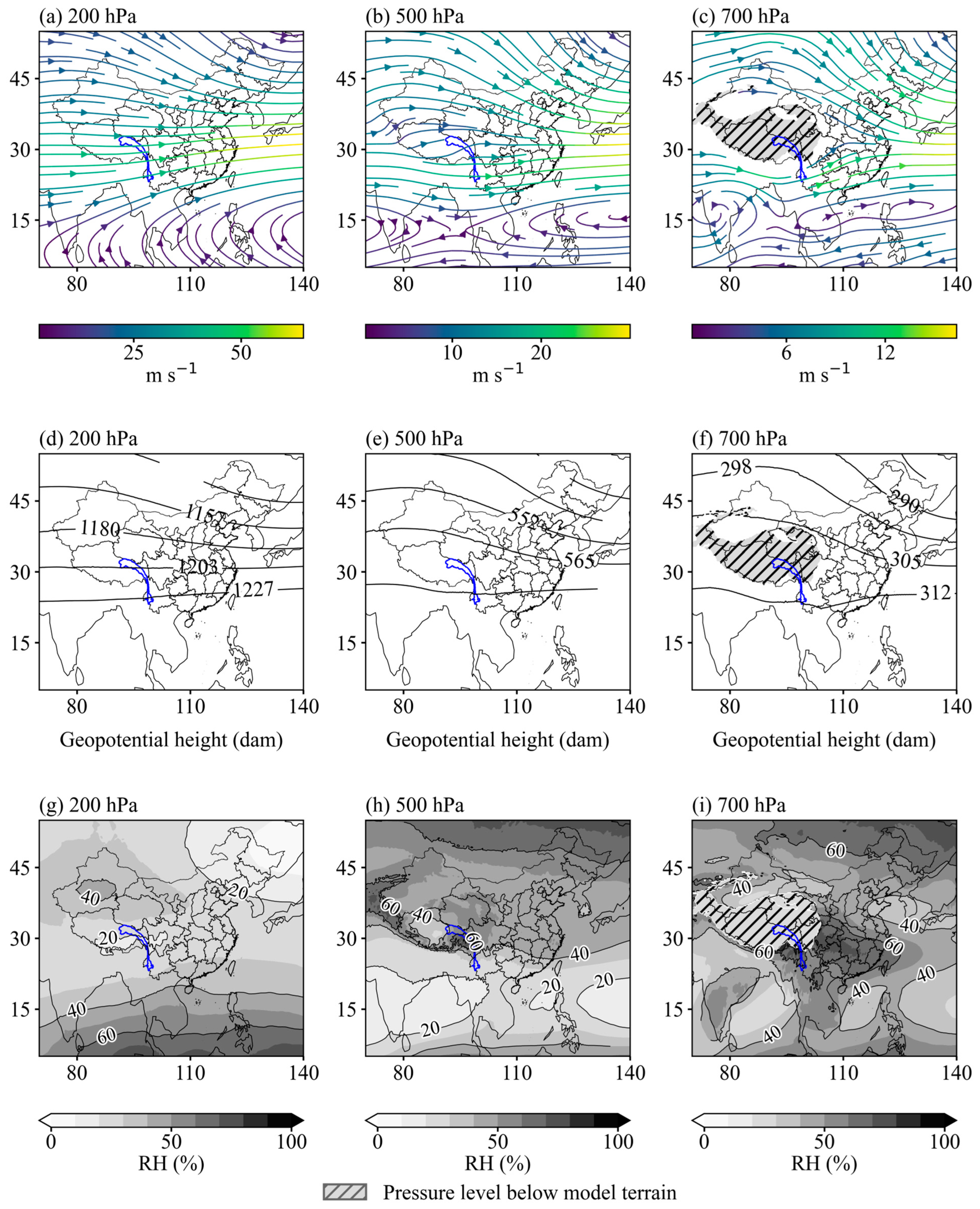
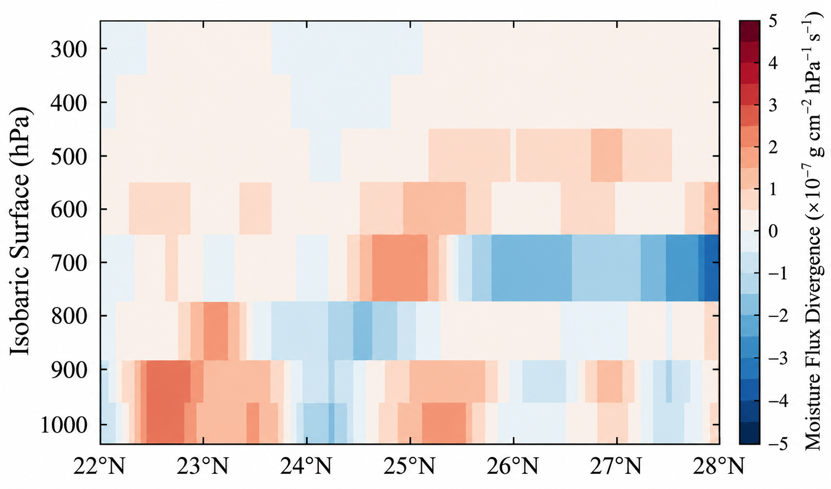
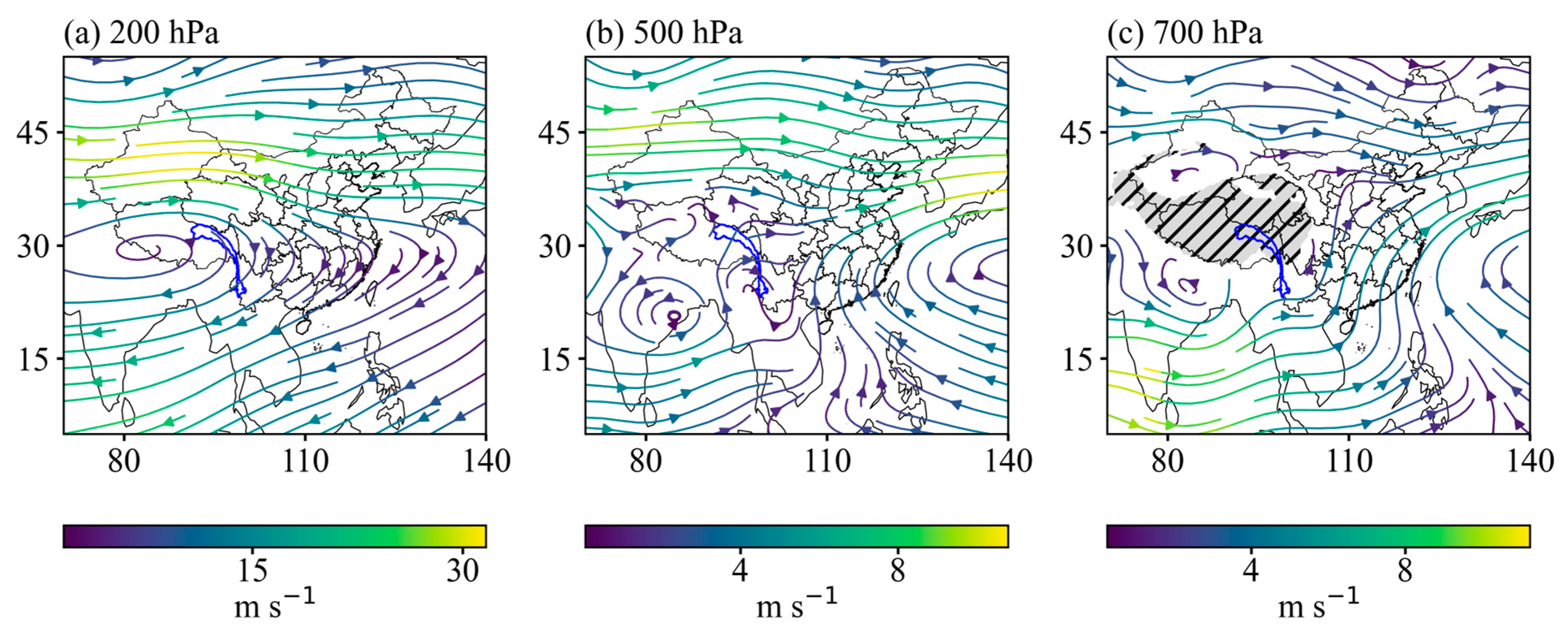
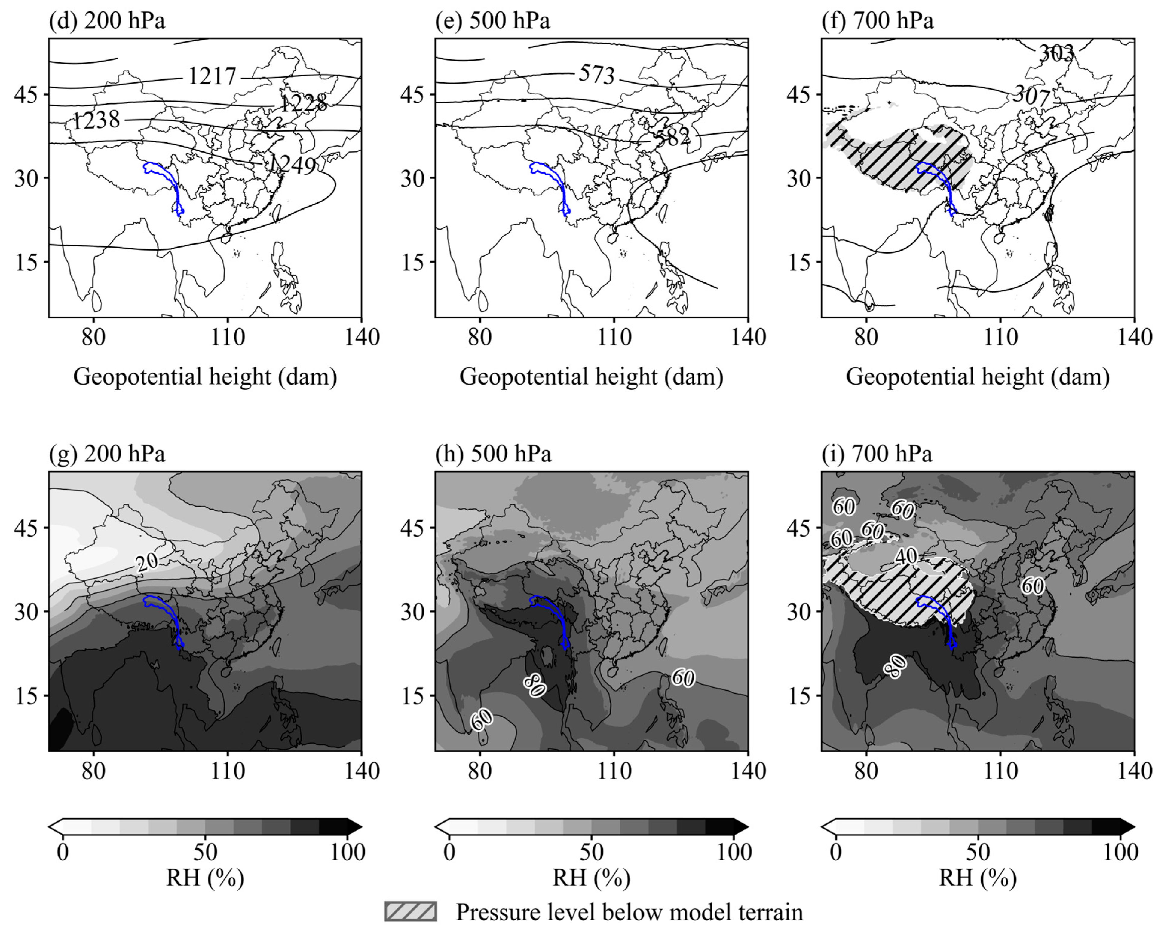
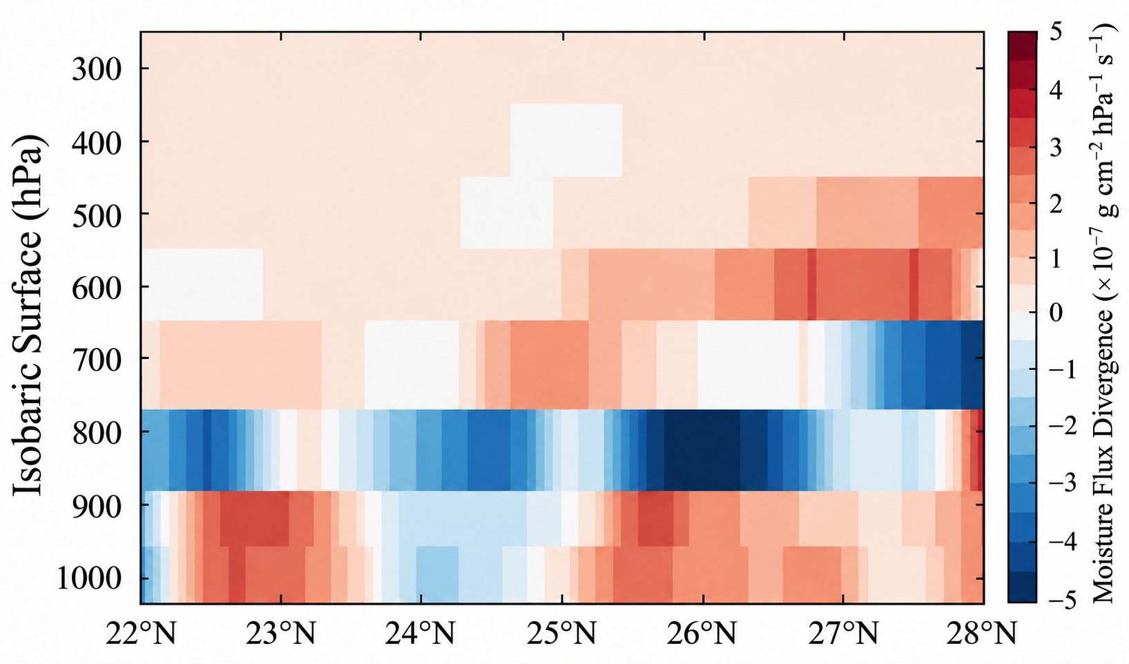
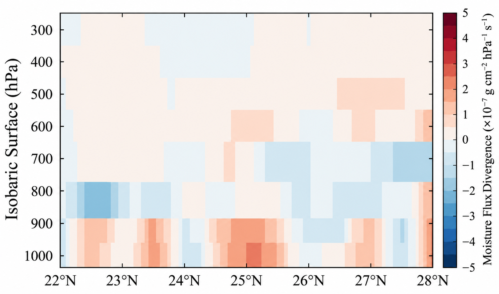
March, July, and October have distinct circulation and humidity backgrounds. In March, the co-located mean zonal wind is 42.47 m s⁻¹ at 200 hPa, 21.17 m s⁻¹ at 500 hPa, and 8.50 m s⁻¹ at 700 hPa. Relative humidity at these levels is 23.89%, 33.38%, and 63.79%, respectively (Table S6). Figure 7 places these local values within the broader westerly circulation over southern Asia. Figure 8 shows convergence in the northern part of the 700 hPa section and divergence near 25° N.

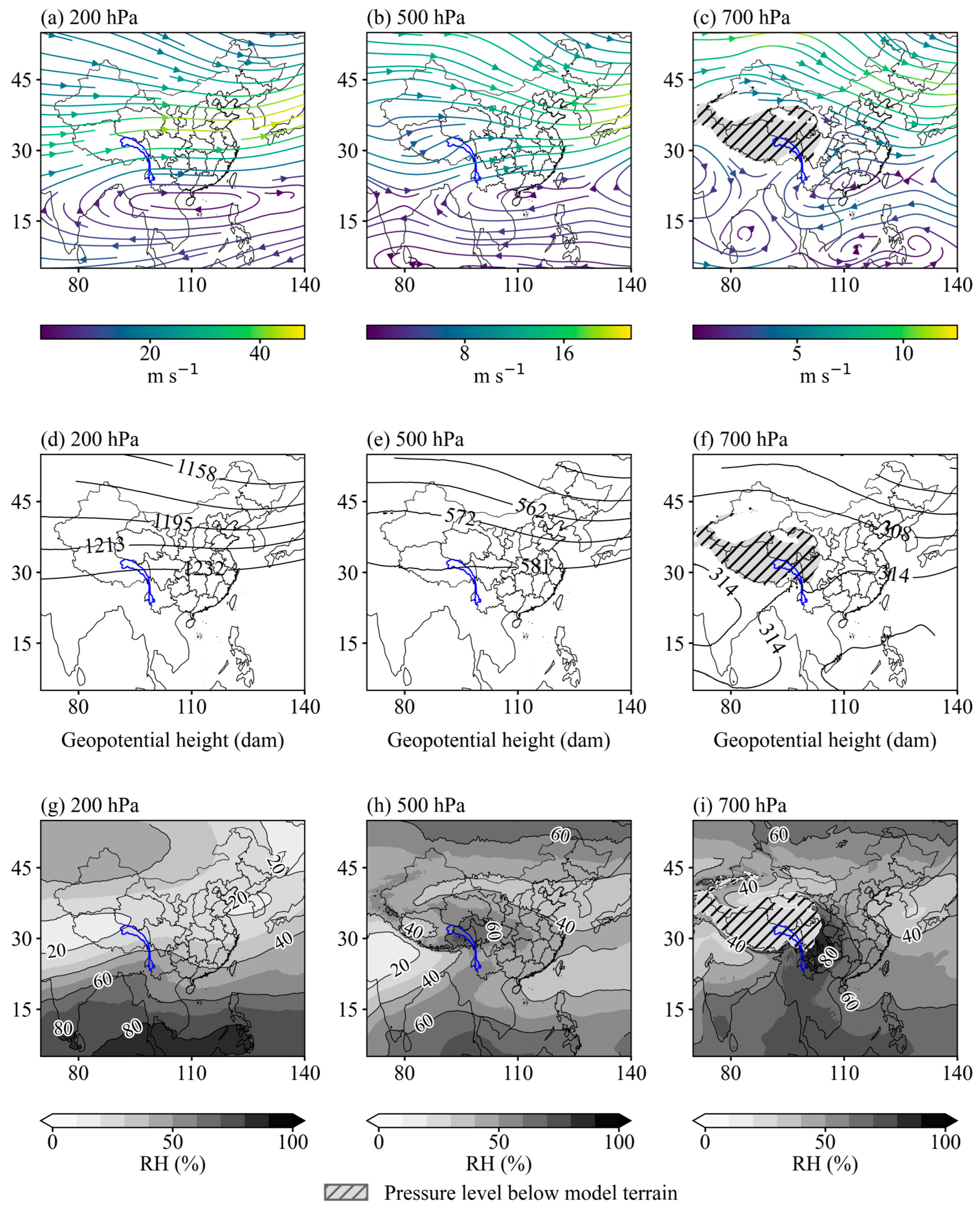
In July, the co-located zonal flow changes to −8.16 m s⁻¹ at 200 hPa, while the 500 and 700 hPa values are 1.08 and 3.60 m s⁻¹. Relative humidity rises to 79.39%, 82.04%, and 90.20% at 200, 500, and 700 hPa, respectively (Figure 9; Table S6). This humid seasonal background coincides with the July maximum in recorded precipitation-day counts. Figure 10 shows stronger convergence around 800–850 hPa than the March section, together with divergence around 600 hPa in the northern part of the section.

October shows a return to upper-level westerly flow: the co-located 200 hPa zonal wind is 16.72 m s⁻¹ (Figure 11). Relative humidity is 49.96%, 52.23%, and 77.42% at 200, 500, and 700 hPa. Compared with July, the 500 hPa humidity decreases by 29.81 pp, and regional R20mm decreases from 4.05 to 1.69 days per month. These circulation and humidity changes accompany the seasonal decrease in precipitation-day counts. The October section shows weaker convergence around 800–850 hPa than in July (Figure 12).

3.2.3. Seasonal and Interannual Variability of the Pressure-Level Wind Field

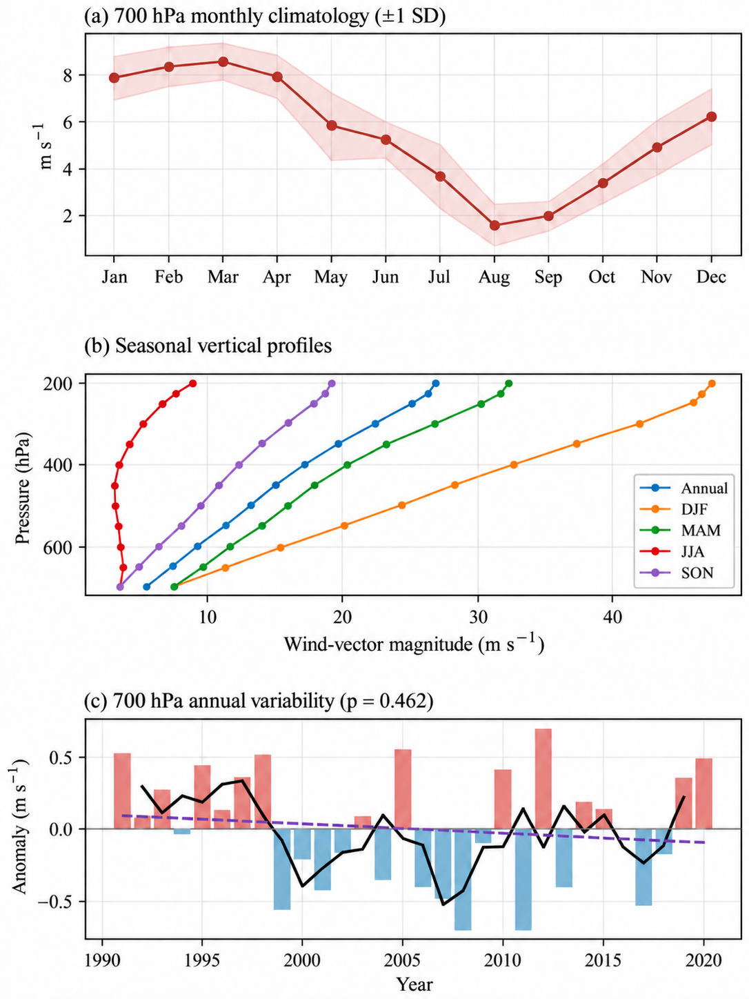
The 700 hPa magnitude calculated from monthly mean wind vectors has a regional climatological maximum of 8.59 m s⁻¹ in March and a minimum of 1.60 m s⁻¹ in August (Figure 13a). The vertical profiles show a stronger increase with height in winter than in summer: at 200 hPa, the DJF and JJA means are 47.19 and 8.78 m s⁻¹, respectively (Figure 13b). The annual 700 hPa series has a mean of 5.47 m s⁻¹ and a trend of −0.06 m s⁻¹ per decade (OLS p = 0.462; Newey–West p = 0.410; Figure 13c; Table S10).

3.3. Extreme-Event Frequencies in ERA5 and Station Records

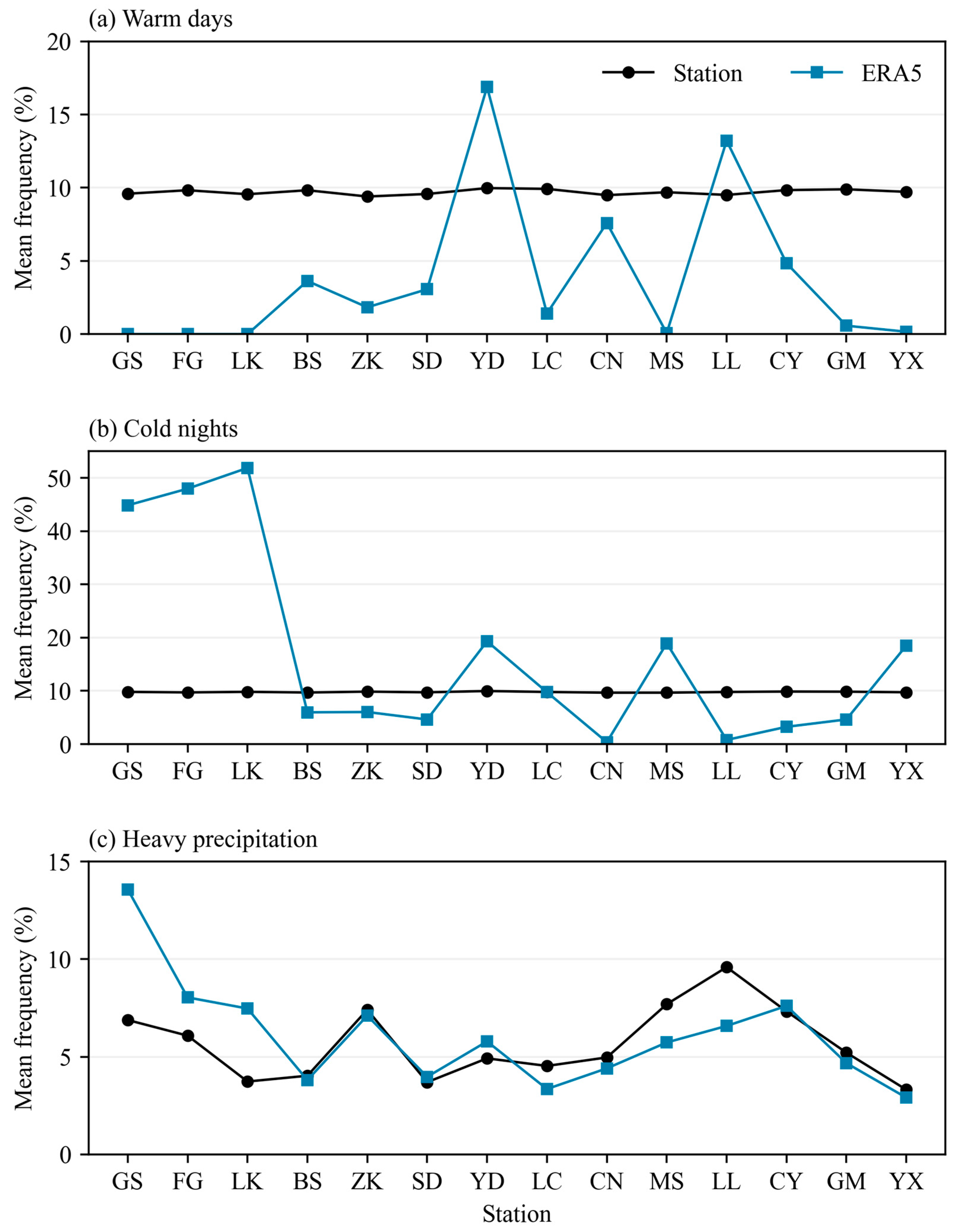
Figure 14 compares station-specific mean event frequencies over 1991–2020;

Table 4. Matched counts and frequencies under common fixed observed temperature thresholds and the ≥20 mm precipitation threshold. Counts use shared valid dates; frequency and count values are equal-weight means across 14 stations and 30 years. Δf is ERA5 minus station frequency (pp). The raw and detrended Pearson correlations (r) compare the 30 annual regional frequency values; detrending applies only to correlation analysis.

Event	Valid Days/yr	Station Days/yr	ERA5 Days/yr	Station (%)	ERA5 (%)	Δf (pp)	r (Raw)	r (Detr.)
Warm days	365.26	35.43	13.90	9.70	3.81	−5.89	0.927	0.887
Cold nights	365.26	35.73	61.80	9.78	16.92	7.14	0.654	0.568
Heavy precipitation	328.73	18.74	19.98	5.67	6.07	0.40	0.695	0.624

summarizes the regional mean frequencies and correlations between the annual regional series. Observed warm-day frequency averages 9.70%, compared with 3.81% in ERA5, a difference of −5.89 pp. Cold-night frequency averages 9.78% in observations and 16.92% in ERA5, a difference of +7.14 pp.

On common numerically recorded precipitation days, the frequency of ≥20 mm precipitation is 5.67% in station data and 6.07% in ERA5, a difference of +0.40 pp. These precipitation comparisons include 138,066 paired station-days, averaging 328.73 valid days per station-year. Mean event counts over those same dates are 18.74 and 19.98 days per year. Table 4 gives the counts and denominators for all three examples, while Table S7 provides results at each station. The regional means summarize a station-dependent pattern of frequency differences visible in Figure 14.

Individual calculations illustrate the station dependence. At Liuku in 2009, the observed TX90 threshold is 32.6 °C: the station records 73/365 warm days (20.00%), and ERA5 records 0/365 (0.00%). Using the observed TN10 threshold of 8.3 °C, cold-night frequencies at the same station are 32/365 (8.77%) and 182/365 (49.86%). At Longling in 2016, precipitation ≥ 20 mm occurs on 36/345 common valid days in the station record (10.43%), and 27/345 in ERA5 (7.83%). Station-specific thresholds, denominators, and frequencies are provided in Table S7.

The two datasets share interannual variation in regional event frequencies, most strongly for warm days. For warm days, cold nights, and heavy-precipitation days, the raw Pearson correlations are 0.927, 0.654, and 0.695, respectively; the corresponding detrended correlations are 0.887, 0.568, and 0.624 (Table 4; Figure S4 and Table S8). All three residual pairs retain positive correlations after removal of their fitted linear trends. Their mean ERA5-minus-observation frequency differences are −5.89, +7.14, and +0.40 pp, respectively. Figure 14 shows how these long-term mean frequencies differ among stations, whereas Figure S4 shows their year-to-year evolution.

The daily comparison shows differences in the dates identified by the two datasets (Figure S5; Table S9). Pooled POD/FAR/CSI values are 0.263/0.329/0.233 for warm days, 0.634/0.633/0.303 for cold nights, and 0.394/0.630/0.236 for heavy-precipitation days. For heavy precipitation, observations identify 7871 station-days, and ERA5 identifies 8390; 3105 are shared, 4766 are identified only by observations, and 5285 only by ERA5. Both datasets classify the remaining 124,910 paired station-days as below 20 mm. Station-specific CSI ranges are 0.000–0.536, 0.036–0.633, and 0.185–0.331 for the three event types, respectively. Complete pooled and station-level counts, including NA values for undefined metrics, are provided in Table S9.

4. Discussion

4.1. Regional Context and Interpretation of the Observed Changes

The high-relief monsoon setting helps organize the contrasting behavior of temperature and precipitation in the Yunnan reach. Across the station network, warm-event frequencies rise and cold-event frequencies fall, while precipitation exhibits strong spatial contrasts and substantial annual variability (Table 3; Figure 2 and Figure 3). This distinction provides the regional context for interpreting the circulation results and the ERA5 comparison.

The observed mean-temperature trend of +0.38 °C per decade remains significant under all five Newey–West lag settings (p < 0.001) and documents warming across the sampled network during 1991–2020. The positive TXx, TNx, and TNn trends and the contrasting warm/cold frequency trends are consistent with this measured change. For global context, IPCC AR6 reports a 2011–2020 global surface temperature approximately 1.09 °C above 1850–1900 [2]. Their direction is also consistent with studies of temperature extremes in China and the Tibetan Plateau [6,9]. Independent analyses also document continued global surface warming during 1973–2022 [29] and rising night-time temperatures in the Canary Islands [30].

The recorded precipitation decline is supported by both conventional OLS and Newey–West inference for this 1991–2020 station network. For PRCPTOT, the lag-one residual autocorrelation is −0.248, and the three-lag Ljung–Box p-value is 0.329. The Newey–West standard error is smaller than the conventional OLS value; accounting for residual covariance does not necessarily widen a confidence interval. The 95% interval of −110.03 to −28.51 mm per decade remains below zero, whereas R² = 0.135 indicates that most annual precipitation variability occurs around the fitted trend. These results describe the network’s recorded wet-day totals over the study period; station-to-station contrasts and interannual variability remain central to their interpretation.

The Longling–Yunxian precipitation contrast and the March–July–October circulation differences are consistent with a role for spatially varying moisture supply in the mountain–valley setting [14,15]. The present station values quantify this contrast: Longling records 2.38 times the wet-day total and 3.09 times the R20mm count at Yunxian. Topographically structured rainfall has also been documented along the Himalaya [31]. The distinction between precipitation totals and daily extremes is central to global comparisons of dry and wet regions [32].

Station observations establish local event thresholds and recorded frequencies, and ERA5 supplies temporally complete hourly fields and a spatial circulation context. Their direct comparison quantifies dataset-dependent behavior: warm days are less frequent and cold nights more frequent in ERA5 under shared observed thresholds, whereas the regional ≥20 mm precipitation contrast is smaller (Table 4). Grid-cell topography, spatial averaging, and hourly sampling are relevant to interpreting these differences [21]. China-wide comparisons likewise identify differences between observational and reanalysis estimates of temperature-extreme changes [33]. Earlier Nujiang evaluations assessed precipitation products using observed discharge [34], while global intercomparisons documented precipitation-estimate differences from daily to annual scales [35].

Temporal covariation and absolute event frequency require separate evaluation. Warm days have the strongest annual correlations among the three examples (raw r = 0.927; detrended r = 0.887), while their mean frequency is 9.70% in observations and 3.81% in ERA5 (Table 4). The station-specific frequency contrasts in Figure 14 describe a different aspect from the annual evolution in Figure S4. Heavy precipitation further illustrates the distinction between frequency and event-date correspondence: its mean frequencies are 5.67% and 6.07%, while its pooled daily CSI is 0.236. Across the three event types, pooled CSI ranges from 0.233 to 0.303. Shared annual variation therefore coexists with differences in mean frequency, its distribution among stations, and the dates of individual extreme days.

The increases in warm-day and warm-night frequencies provide a quantitative basis for local heat monitoring [36], while the range of precipitation indices supports attention to station-specific rainfall conditions. Studies of ecosystem sensitivity to water and energy conditions in China provide an ecological context for these temperature and precipitation summaries [37]. ERA5 WSx and W95d add a clearly defined description of hourly resolved near-surface wind extremes.

4.2. Circulation Associations and Dry/Wet Examples

4.2.1. Monsoon and Pacific Indices

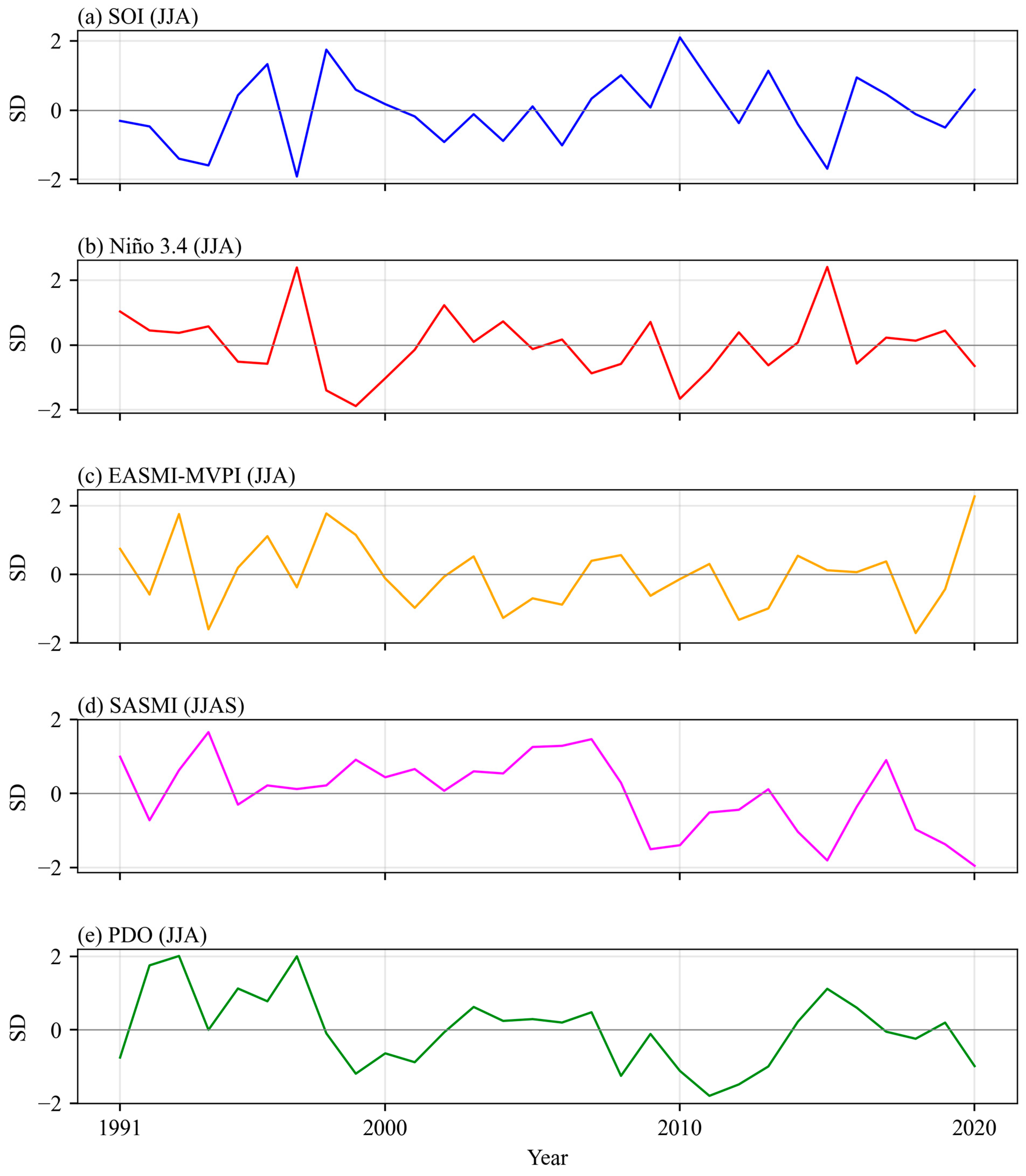
Figure 15 shows the five circulation indices, standardized only for visual comparison. The statistical calculations retain the source-defined seasonal series: JJAS for SASMI and JJA for EASMI-MVPI, SOI, Niño 3.4, and PDO. Table S4 reports the complete raw and detrended correlation results with their p- and q-values.

The largest raw associations include SASMI–TN90p (r = −0.557, p = 0.0014), SASMI–TNx (r = −0.536, p = 0.0023), and PDO–TX10p (r = 0.551, p = 0.0016). Each has q = 0.045 across the 60 raw tests. In contrast, SASMI–PRCPTOT is positive but not significant (r = 0.312, p = 0.094). After controlling for a linear time trend, SASMI–TN90p is −0.202 (p = 0.293), and PDO–TX10p is 0.450 (p = 0.014). No detrended association meets q < 0.05. Thus, these raw associations include shared long-term variation; their detrended counterparts describe residual interannual covariation between the summer state and the same year’s annual index.

The PDO calculation adds North Pacific variability to the monsoon and ENSO comparison, following its established interpretation as a pattern arising from several interacting processes [25]. Here, JJA PDO is used as a concurrent seasonal covariate over 1991–2020. ENSO–East Asian teleconnections provide a wider circulation context [17,38]. Indian summer monsoon variability has been linked to the South Asian High and rainfall over China [39], while circulation-budget analyses over the middle and lower Yangtze connect quasi-biweekly rainfall variability with vorticity and divergence [40]. The seasonal SASMI sensitivity results are included alongside the main correlation table so that the consequences of the averaging window remain explicit.

The seasonal–annual associations describe between-year covariation, not a direct response of every event to summer circulation. This distinction is especially relevant to cold-event indices, whose observed occurrence peaks in January, before the summer index is measured, and to warm-day frequency, which peaks in May. An association can combine seasonal persistence, shared trends, and the contribution of other months to the annual total. Detrending removes a linear common time component, but neither detrending nor multiple-testing adjustment identifies a physical mechanism. The two July examples add descriptions of coincident circulation and precipitation anomalies; they are selected cases rather than a composite assessment of dry or wet years.

4.2.2. A Dry Example: July 2009

In 2009, regional recorded PRCPTOT is 1036.99 mm, 21.05% below its 1991–2020 mean. July precipitation is 202.76 mm, 21.95% below the July mean (

Table 5. Recorded precipitation in the selected dry and wet examples. Annual and July anomalies use their respective 1991–2020 regional means.

Year	PRCPTOT (mm)	Annual Anomaly (%)	July Precipitation (mm)	July Anomaly (%)	R20mm (Days)
2009	1036.99	−21.05	202.76	−21.95	15.64
2016	1527.01	16.26	296.36	14.08	23.00

).

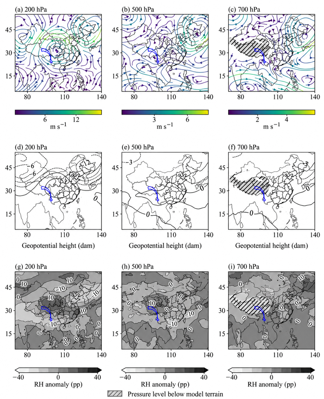
Figure 16 shows July 2009 anomalies from the July climatology. Co-located relative-humidity anomalies are −10.96 and −5.59 pp at 200 and 500 hPa, respectively, while the 700 hPa anomaly is +2.02 pp (Table S6). The zonal-wind anomalies are −6.75, −0.55, and +0.62 m s⁻¹ at 200, 500, and 700 hPa; the corresponding height anomalies are +23.92, +3.01, and −4.66 m. The dry month combines reduced humidity at 200 and 500 hPa with a small positive anomaly at 700 hPa.

4.2.3. A Wet Example: July 2016

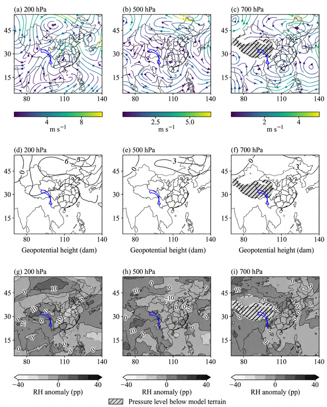
The 2016 regional recorded PRCPTOT is 1527.01 mm, 16.26% above the long-term mean. July precipitation reaches 296.36 mm, 14.08% above the July mean, and annual R20mm is 23.00 days (Table 5). Figure 17 shows the accompanying circulation anomalies. The co-located 700 hPa meridional-wind anomaly is +0.56 m s⁻¹, compared with −0.31 m s⁻¹ in July 2009. Relative-humidity anomalies are +3.49, +0.06, and +0.73 pp at 200, 500, and 700 hPa, respectively, while geopotential-height anomalies are positive at all three levels (+15.88, +13.48, and +13.92 m; Table S6).

Annual TN90p and TX90p in 2016 are 12.90% and 11.67%, respectively, both above their full-period means. Above-average annual precipitation therefore coexists with elevated warm-event frequencies in this year.

4.3. Limitations

The 14-station network samples local environments within and around the Yunnan reach, while the 0.25° ERA5 fields represent grid-scale terrain and atmospheric conditions. Point-to-grid differences in elevation, spatial support, and hourly sampling affect the common-threshold frequency comparison. ERA5 values were used without bias correction or lapse-rate adjustment, so the reported differences include systematic local offsets as well as differences in event occurrence. Thirty annual values constrain the precision of trend and correlation estimates and the detection of temporal dependence. Newey–West inference addresses short-range residual covariance; its finite-sample p-values and intervals remain approximate and depend on the lag setting. Trend tests are pointwise, and correlated station records do not provide independent spatial replications. Correlation p- and q-values use the stated parametric reference distributions; detrending and false-discovery-rate adjustment do not correct residual serial dependence or the mismatch between seasonal predictors and annual outcomes. Circulation associations and the selected dry and wet cases are exploratory descriptions of covariation and accompanying conditions, rather than causal attribution or estimates representative of all such events.

5. Conclusions

Daily observations from 14 stations and ERA5 fields document temperature, precipitation, and wind extremes in and around the Yunnan reach of the Nujiang River Basin during 1991–2020. The regional annual maximum of daily maximum temperature (TXx), annual maximum of daily minimum temperature (TNx), and annual minimum of daily minimum temperature (TNn) rise by 0.50, 0.39, and 0.55 °C per decade. Warm-night and warm-day frequencies increase by 3.98 and 3.00 pp per decade, while cold-night and cold-day frequencies decrease by 2.67 and 2.87 pp per decade. These changes accompany an observed mean-temperature increase of 0.38 °C per decade. The seven temperature-extreme trends listed above, and the mean-temperature trend, remain significant in Newey–West tests, with maximum lags of one to five years (all p < 0.005).

Recorded wet-day precipitation has a station-network mean of 1313.48 mm and a fitted trend of −69.27 mm per decade (OLS p = 0.045; Newey–West p = 0.0017; 95% confidence interval: −110.03 to −28.51 mm per decade). This decline remains significant across the tested lag settings, while the linear trend explains 13.5% of the annual variance. Climatological values range from 847.46 mm at Yunxian to 2016.39 mm at Longling. The frequency of ≥20 mm precipitation peaks regionally in July at 4.05 recorded days per month. ERA5 annual maximum hourly 10 m wind speed averages 4.62 m s⁻¹, and neither this index nor its 95th-percentile exceedance-day count has a significant trend under either conventional OLS or Newey–West tests.

Applying the same fixed observed temperature thresholds (the 90th percentile of daily maximum temperature for warm days and the 10th percentile of daily minimum temperature for cold nights) to both datasets yields ERA5-minus-station frequency differences of −5.89 pp for warm days, +7.14 for cold nights, and +0.40 for ≥20 mm precipitation on matched valid dates. Seasonal humidity and wind fields provide a quantitative circulation context for the Yunnan reach. The seasonal-index correlations describe concurrent covariation with annual indices, and the two July cases illustrate accompanying circulation conditions. Three raw circulation–temperature associations meet the Benjamini–Hochberg false-discovery-rate criterion (adjusted p-value, q < 0.05); none meet this criterion after removing linear trends. The resulting picture combines a clear shift in temperature extremes with spatially differentiated precipitation and distinct reanalysis frequency behavior.

References

1. Seneviratne, S.I.; Nicholls, N.; Easterling, D.; Goodess, C.M.; Kanae, S.; Kossin, J.; Luo, Y.; Marengo, J.; McInnes, K.; Rahimi, M.; et al. Changes in climate extremes and their impacts on the natural physical environment. In Managing the Risks of Extreme Events and Disasters to Advance Climate Change Adaptation; Field, C.B., Barros, V., Stocker, T.F., Qin, D., Dokken, D.J., Ebi, K.L., Mastrandrea, M.D., Mach, K.J., Plattner, G.-K., Allen, S.K., et al., Eds.; Cambridge University Press: Cambridge, UK; New York, NY, USA, 2012; pp. 109–230. [Google Scholar]
2. IPCC. Climate Change 2021: The Physical Science Basis. In Contribution of Working Group I to the Sixth Assessment Report of the Intergovernmental Panel on Climate Change; Masson-Delmotte, V., Zhai, P., Pirani, A., Connors, S.L., Péan, C., Berger, S., Caud, N., Chen, Y., Goldfarb, L., Gomis, M.I., et al., Eds.; Cambridge University Press: Cambridge, UK; New York, NY, USA, 2021. [Google Scholar] [CrossRef] [Scilit]
3. Zhang, X.; Alexander, L.; Hegerl, G.C.; Jones, P.; Klein Tank, A.M.G.; Peterson, T.C.; Trewin, B.; Zwiers, F.W. Indices for monitoring changes in extremes based on daily temperature and precipitation data. WIREs Clim. Change 2011, 2, 851–870. [Google Scholar] [CrossRef] [Scilit]
4. Li, X.; Li, X.; Hua, W.; Ma, H.; Zhou, J.; Pang, X. Modeling the effects of present-day irrigation on temperature extremes over China. Front. Earth Sci. 2023, 11, 1084892. [Google Scholar] [CrossRef] [Scilit]
5. Zhang, D.-L. Rapid urbanization and more extreme rainfall events. Sci. Bull. 2020, 65, 516–518. [Google Scholar] [CrossRef] [Scilit]
6. Zhao, N.; Chen, M. A comprehensive study of spatiotemporal variations in temperature extremes across China during 1960–2018. Sustainability 2021, 13, 3807. [Google Scholar] [CrossRef] [Scilit]
7. Wang, X.; Wu, L.; Liu, H. Extreme temperature index in China from a statistical perspective: Change characteristics and trend analysis from 1961 to 2021. Atmosphere 2024, 15, 1398. [Google Scholar] [CrossRef] [Scilit]
8. Wang, B.; Gao, M.; Li, Y.; Xu, H.; Li, Z.; Peng, J. Spatiotemporal trends of extreme temperature events along the Qinghai–Tibet Plateau transportation corridor from 1981 to 2019 based on estimated near-surface air temperature. J. Geophys. Res. Atmos. 2023, 128, e2023JD039040. [Google Scholar] [CrossRef] [Scilit]
9. Yang, K.; Guo, D.; Hua, W.; Pepin, N.; Yang, K.; Li, D. Tibetan Plateau temperature extreme changes and their elevation dependency from ground-based observations. J. Geophys. Res. Atmos. 2022, 127, e2021JD035734. [Google Scholar] [CrossRef] [Scilit]
10. You, Q.; Chen, D.; Wu, F.; Pepin, N.; Cai, Z.; Ahrens, B.; Jiang, Z.; Wu, Z.; Kang, S.; AghaKouchak, A. Elevation dependent warming over the Tibetan Plateau: Patterns, mechanisms and perspectives. Earth-Sci. Rev. 2020, 210, 103349. [Google Scholar] [CrossRef] [Scilit]
11. Chen, W.; Cui, H.; Zwiers, F.W.; Li, C.; Zheng, J. Detection and attribution of changes in precipitation extremes in China and its different climate zones. J. Clim. 2024, 37, 5373–5385. [Google Scholar] [CrossRef] [Scilit]
12. Zhao, D.; Xu, H.; Li, Y.; Yu, Y.; Duan, Y.; Xu, X.; Chen, L. Locally opposite responses of the 2023 Beijing–Tianjin–Hebei extreme rainfall event to global anthropogenic warming. npj Clim. Atmos. Sci. 2024, 7, 38. [Google Scholar] [CrossRef] [Scilit]
13. Miao, L.; Ju, L.; Sun, S.; Agathokleous, E.; Wang, Q.; Zhu, Z.; Liu, R.; Zou, Y.; Lu, Y.; Liu, Q. Unveiling the dynamics of sequential extreme precipitation–heatwave compounds in China. npj Clim. Atmos. Sci. 2024, 7, 67. [Google Scholar] [CrossRef] [Scilit]
14. Fan, H.; He, D. Regional climate and its change in the Nujiang River Basin. Acta Geogr. Sin. 2012, 67, 621–630. (In Chinese) [Google Scholar]
15. Pan, F.; He, D.; Cao, J.; Lu, Y. Multiple branches of water vapor transport over the Nujiang River Basin in summer and its impact on precipitation. Acta Geogr. Sin. 2023, 78, 87–100. [Google Scholar]
16. Tian, S.; Dai, G.; Yin, Q.; Meng, X.; Zhang, Z.; Zhu, Z.; Xiao, G. Spatial differences in East Asian climate transition at ~260 ka and their links to ENSO. Quat. Sci. Rev. 2022, 296, 107805. [Google Scholar] [CrossRef] [Scilit]
17. Serykh, I.V.; Sonechkin, D.M.; Byshev, V.I.; Neiman, V.G.; Romanov, Y.A. Global Atmospheric Oscillation: An Integrity of ENSO and Extratropical Teleconnections. Pure Appl. Geophys. 2019, 176, 3737–3755. [Google Scholar] [CrossRef] [Scilit]
18. Ji, X.; Chen, Y.; Jiang, W.; Liu, C.; Yang, L. Glacier area changes in the Nujiang–Salween River Basin over the past 45 years. J. Geogr. Sci. 2022, 32, 1177–1204. [Google Scholar] [CrossRef] [Scilit]
19. Chai, C.; Wang, L.; Chen, D.; Zhou, J.; Liu, H.; Zhang, J.; Wang, Y.; Chen, T.; Liu, R. Future snow changes and their impact on the upstream runoff in Salween. Hydrol. Earth Syst. Sci. 2022, 26, 4657–4683. [Google Scholar] [CrossRef] [Scilit]
20. Li, Y.; Zhao, J.; Yuan, J.; Ji, P.; Deng, X.; Yang, Y. Constructing the ecological security pattern of Nujiang Prefecture based on the framework of “Importance–Sensitivity–Connectivity”. Int. J. Environ. Res. Public Health 2022, 19, 10869. [Google Scholar] [CrossRef] [Scilit]
21. Hersbach, H.; Bell, B.; Berrisford, P.; Hirahara, S.; Horányi, A.; Muñoz-Sabater, J.; Nicolas, J.; Peubey, C.; Radu, R.; Schepers, D.; et al. The ERA5 global reanalysis. Q. J. R. Meteorol. Soc. 2020, 146, 1999–2049. [Google Scholar] [CrossRef] [Scilit]
22. Li, J.; Zeng, Q. A unified monsoon index. Geophys. Res. Lett. 2002, 29, 115-1–115-4. [Google Scholar] [CrossRef] [Scilit]
23. Yang, Y.-N.; Li, J.-P. Novel monsoon indices based on vector projection and directed angle for measuring the East Asian summer monsoon. Clim. Dyn. 2025, 63, 210. [Google Scholar] [CrossRef] [Scilit]
24. Mir, S.; Arbab, M.A.; Rehman, S.U. ENSO dataset & comparison of deep learning models for ENSO forecasting. Earth Sci. Inform. 2024, 17, 2623–2628. [Google Scholar] [CrossRef] [Scilit]
25. Newman, M.; Alexander, M.A.; Ault, T.R.; Cobb, K.M.; Deser, C.; Di Lorenzo, E.; Mantua, N.J.; Miller, A.J.; Minobe, S.; Nakamura, H.; et al. The Pacific Decadal Oscillation, Revisited. J. Clim. 2016, 29, 4399–4427. [Google Scholar] [CrossRef] [Scilit]
26. Ljung, G.M.; Box, G.E.P. On a measure of lack of fit in time series models. Biometrika 1978, 65, 297–303. [Google Scholar] [CrossRef]
27. Newey, W.K.; West, K.D. A simple, positive semi-definite, heteroskedasticity and autocorrelation consistent covariance matrix. Econometrica 1987, 55, 703–708. [Google Scholar] [CrossRef] [Scilit]
28. Benjamini, Y.; Hochberg, Y. Controlling the false discovery rate: A practical and powerful approach to multiple testing. J. R. Stat. Soc. B 1995, 57, 289–300. [Google Scholar] [CrossRef] [Scilit]
29. Samset, B.H.; Zhou, C.; Fuglestvedt, J.S.; Lund, M.T.; Marotzke, J.; Zelinka, M.D. Steady global surface warming from 1973 to 2022 but increased warming rate after 1990. Commun. Earth Environ. 2023, 4, 400. [Google Scholar] [CrossRef] [Scilit]
30. Correa, J.; López-Díez, A.; Dorta, P.; Díaz-Pacheco, J. Evolution of warm nights in the Canary Islands (1950–2023): Evidence for climate change in the Southeastern North Atlantic. Theor. Appl. Climatol. 2025, 156, 87. [Google Scholar] [CrossRef] [Scilit]
31. Bookhagen, B.; Burbank, D.W. Toward a complete Himalayan hydrological budget: Spatiotemporal distribution of snowmelt and rainfall and their impact on river discharge. J. Geophys. Res. Earth Surf. 2010, 115, F03019. [Google Scholar] [CrossRef] [Scilit]
32. Donat, M.G.; Lowry, A.L.; Alexander, L.V.; O’Gorman, P.A.; Maher, N. More extreme precipitation in the world’s dry and wet regions. Nat. Clim. Change 2016, 6, 508–513. [Google Scholar] [CrossRef] [Scilit]
33. Zhao, S.; Zhou, T.; Chen, X. Consistency of extreme temperature changes in China under a historical half-degree warming increment across different reanalysis and observational datasets. Clim. Dyn. 2020, 54, 2465–2479. [Google Scholar] [CrossRef] [Scilit]
34. Mao, R.; Wang, L.; Zhou, J.; Li, X.; Qi, J.; Zhang, X. Evaluation of various precipitation products using ground-based discharge observation at the Nujiang River Basin, China. Water 2019, 11, 2308. [Google Scholar] [CrossRef] [Scilit]
35. Sun, Q.; Miao, C.; Duan, Q.; Ashouri, H.; Sorooshian, S.; Hsu, K.-L. A review of global precipitation data sets: Data sources, estimation, and intercomparisons. Rev. Geophys. 2018, 56, 79–107. [Google Scholar] [CrossRef] [Scilit]
36. Zhao, F.; Zhang, M.; Zhu, S.; Zhang, X.; Ma, S.; Gao, Y.; Xia, J.; Wang, X.; Zhang, Y.; Zhang, S.; et al. Spatiotemporal patterns of the urban thermal environment and the impact of human activities in low-latitude plateau cities. Int. J. Appl. Earth Obs. Geoinf. 2025, 142, 104703. [Google Scholar] [CrossRef] [Scilit]
37. Hu, Y.; Wei, F.; Fu, B.; Zhang, W.; Sun, C. Ecosystems in China have become more sensitive to changes in water demand since 2001. Commun. Earth Environ. 2023, 4, 444. [Google Scholar] [CrossRef] [Scilit]
38. Wang, B.; Wu, R.; Fu, X. Pacific–East Asian teleconnection: How does ENSO affect East Asian climate? J. Clim. 2000, 13, 1517–1536. [Google Scholar] [CrossRef] [Scilit]
39. Wei, W.; Zhang, R.; Wen, M.; Rong, X.; Li, T. Impact of Indian summer monsoon on the South Asian High and its influence on summer rainfall over China. Clim. Dyn. 2014, 43, 1257–1269. [Google Scholar] [CrossRef] [Scilit]
40. Liu, Y.; Yao, S.; Shi, Y. Dynamic processes and mechanisms of the quasi-biweekly oscillation of summer precipitation in the middle and lower reaches of the Yangtze River. Atmos. Res. 2026, 330, 108606. [Google Scholar] [CrossRef] [Scilit]
Figure 2. Climatological means (1991–2020) of the 12 station indices: (ad) annual temperature extremes; (eh) percentile temperature-event frequencies; and (il) precipitation indices. Colors indicate station values, with units shown in each panel title. Black and blue lines show province boundaries and rivers. All panels use the same north-up extent (97.30–101.50° E, 22.80–28.15° N). Longitude and latitude are labeled on every panel. Station abbreviations are placed inside each map and defined in Table 1; the geographical context is shown in Figure 1.
Geosciences 16 00382 g002
Figure 3. Regional annual anomalies of the 12 station indices: (ad) annual temperature extremes; (eh) percentile temperature-event frequencies; and (il) precipitation indices. Light blue bars show anomalies relative to the 1991–2020 mean, red lines show centered 3-year running means, and black dashed lines show linear trends fitted to the unsmoothed annual series. pp denotes percentage points. Trend estimates and tests are listed in Table 3.
Geosciences 16 00382 g003
Figure 4. ERA5-derived 10 m wind extremes at the 14 co-located grid cells: (a) mean of the local annual maximum hourly speeds (WSx); (b) mean annual count of days whose daily maximum hourly speed exceeds the cell-specific fixed 1991–2020 95th percentile (W95d); and (c) climatological mean monthly exceedance-day counts. Blue lines with markers in panels (a,b) show the annual regional mean values, and red dashed lines show linear trends fitted to the unsmoothed annual series.“High-wind days” in panels (b,c) are days meeting this W95d threshold; the cell-specific thresholds range from 1.95 to 4.48 m s−1 (Table S5). The p-values annotated in the figure are from conventional OLS tests; Newey–West results are reported in Table S10.
Geosciences 16 00382 g004
Figure 5. Cumulative monthly counts of (a) cold nights (TN10p), (b) cold days (TX10p), (c) warm nights (TN90p), and (d) warm days (TX90p) at the 14 stations over 1991–2020. Counts use the fixed annual-baseline temperature thresholds. Months 1–12 denote January–December. Dividing each plotted count by 30 gives the climatological mean monthly count. Station information is provided in Table 1.
Geosciences 16 00382 g005
Figure 6. Cumulative monthly counts of (a) wet days (>1 mm), (b) R10mm (≥10 mm), and (c) R20mm (≥20 mm)at the 14 stations over 1991–2020. Months 1–12 denote January–December. Dividing each count by 30 gives the climatological mean monthly count. Station information is provided in Table 1.
Geosciences 16 00382 g006
Figure 7. Climatological March circulation, 1991–2020. Columns show 200, 500, and 700 hPa, respectively. Panels (ac) show wind streamlines colored by speed (m s−1), panels (df) show geopotential-height contours (dam), and panels (gi) show relative humidity (%). The blue outline marks the Nujiang basin. Gray hatching marks grid cells where the pressure level lies beneath the ERA5 model terrain; these cells are excluded from the plotted fields. Humidity is shown with a grayscale and labeled contours.
Geosciences 16 00382 g007
Figure 8. Pressure–latitude cross-section of moisture-flux divergence along 98° E for March, based on the 1991–2020 monthly climatology. Negative and positive values indicate convergence and divergence, respectively (g cm−2 hPa−1 s−1).
Geosciences 16 00382 g008
Figure 9. Climatological July circulation, 1991–2020. Columns show 200, 500, and 700 hPa, respectively. Panels (ac) show wind streamlines colored by speed (m s−1), panels (df) show geopotential-height contours (dam), and panels (gi) show relative humidity (%). The blue outline marks the Nujiang basin. Gray hatching marks grid cells where the pressure level lies beneath the ERA5 model terrain; these cells are excluded from the plotted fields. Humidity is shown with a grayscale and labeled contours.
Geosciences 16 00382 g009aGeosciences 16 00382 g009b
Figure 10. Pressure–latitude cross-section of moisture-flux divergence along 98° E for July, based on the 1991–2020 monthly climatology. Negative and positive values indicate convergence and divergence, respectively (g cm−2 hPa−1 s−1).
Geosciences 16 00382 g010
Figure 11. Climatological October circulation, 1991–2020. Columns show 200, 500, and 700 hPa, respectively. Panels (ac) show wind streamlines colored by speed (m s−1), panels (df) show geopotential-height contours (dam), and panels (gi) show relative humidity (%). The blue outline marks the Nujiang basin. Gray hatching marks grid cells where the pressure level lies beneath the ERA5 model terrain; these cells are excluded from the plotted fields. Humidity is shown with a grayscale and labeled contours.
Geosciences 16 00382 g011
Figure 12. Pressure–latitude cross-section of moisture-flux divergence along 98° E for October, based on the 1991–2020 monthly climatology. Negative and positive values indicate convergence and divergence, respectively (g cm−2 hPa−1 s−1).
Geosciences 16 00382 g012
Figure 13. Background wind-vector magnitudes from monthly ERA5 pressure-level fields: (a) 700 hPa monthly climatology, shown by the solid line with markers, with shading indicating ±1 interannual standard deviation; (b) annual and seasonal vertical profiles, with blue, orange, green, red and purple solid lines representing Annual, DJF, MAM, JJA and SON, respectively; and (c) annual 700 hPa anomalies, with red and blue bars indicating positive and negative anomalies, respectively. The black solid line in panel (c) shows the centred three-year moving mean, and the purple dashed line shows the linear trend fitted to the unsmoothed annual series. Seasonal abbreviations are defined in Section 2.3.4. The p-values annotated in panel (c) is from the conventional OLS slope test; Newey–West results are reported in Table S10.
Geosciences 16 00382 g013
Figure 14. Station-specific mean event frequencies during 1991–2020 for (a) warm days above observed TX90 thresholds, (b) cold nights below observed TN10 thresholds, and (c) precipitation ≥ 20 mm. Both datasets use the same valid dates and thresholds at each station. Temperature thresholds are fixed percentiles of the full-period station observations, whose mean exceedance frequencies are consequently close to 10%. Panels (ac) use vertical scales of 0–20%, 0–55%, and 0–15%, respectively. The larger range in (b) includes the maximum cold-night frequency of 51.87%. The horizontal axis lists stations (Table 1); annual regional frequency curves are shown in Figure S4.
Geosciences 16 00382 g014
Figure 15. Source-defined seasonal circulation indices during 1991–2020: (a) SOI, shown in blue; (b) Niño 3.4, shown in red; (c) EASMI-MVPI, shown in orange; (d) SASMI, shown in magenta; and (e) PDO, shown in green. The colored solid lines show the standardized index values, and the grey horizontal line denotes zero standard deviation. Values are standardized relative to their own 30-year means and sample standard deviations for display. SASMI uses JJAS; SOI, Niño 3.4, EASMI-MVPI and PDO use JJA. Statistical calculations use the original seasonal series.
Geosciences 16 00382 g015
Figure 16. July 2009 anomalies relative to the 1991–2020 July mean. Columns show 200, 500, and 700 hPa. Panels (ac) show anomalous wind streamlines colored by magnitude (m s−1), panels (df) show geopotential-height anomalies (dam), and panels (gi) show relative-humidity anomalies (pp). The blue outline marks the Nujiang basin. Gray hatching marks grid cells where the pressure level lies beneath the ERA5 model terrain; these cells are excluded from the plotted fields. Humidity is shown with a grayscale and labeled contours.
Geosciences 16 00382 g016
Figure 17. July 2016 anomalies relative to the 1991–2020 July mean. Columns show 200, 500, and 700 hPa. Panels (ac) show anomalous wind streamlines colored by magnitude (m s−1), panels (df) show geopotential-height anomalies (dam), and panels (gi) show relative-humidity anomalies (pp). The blue outline marks the Nujiang basin. Gray hatching marks grid cells where the pressure level lies beneath the ERA5 model terrain; these cells are excluded from the plotted fields. Humidity is shown with a grayscale and labeled contours.
Geosciences 16 00382 g017