Spatial Modelling of Groundwater Potential Zones Using GIS-Based Machine Learning Techniques: A Case Study of Abuja, Nigeria

Abstract

In many African nations, including Nigeria, groundwater remains the most readily available source of clean water. However, finding and developing these resources in heterogeneous terrain, such as the Federal Capital Territory (FCT), Abuja, is challenging due to the uneven distribution of the aquifers and complex geological settings. Using a GIS-based machine learning approach that incorporates surface and subsurface hydrogeological parameters, this study defines groundwater potential zones (GWPZ). Nine conditioning factors were derived from remote sensing, geophysical and climatic datasets. Aquifer thickness, depth to bedrock, geology, rainfall, slope, LULC, lineament density, drainage density and distance from river were among these variables. Three machine learning models: Extreme Gradient Boosting (XGBoost), Support Vector Machine (SVM) and Random Forest (RF) were trained and validated using 2410 borehole records (productive and abortive). Hold-out validation (80:20), 10-fold cross-validation, ROC-AUC, and confusion matrix were used to assess each model’s performance. The ensemble models outperformed the SVM, achieving higher predictive accuracy and better generalisation (XGBoost: 0.89, RF: 0.88 and SVM: 0.87). The generated maps categorised the study area into five GWPZs: very high, high, moderate, low and very low. These findings provide a scientific foundation for groundwater exploration and sustainable water resource management in the study area.

1. Introduction

About 60% of freshwater extracted worldwide comes from groundwater, which is also the main source of water for homes, industrial and agricultural activities, especially in developing countries. It is therefore a significant freshwater resource on Earth. The possibility that groundwater will occur in a given hydrogeological setting is known as groundwater potential [1]. Groundwater is crucial for maintaining water security and realising the Sustainable Development Goals (SDGs) in many developing nations.

Groundwater remains under stress due to excessive extraction, despite accounting for around 26% of the world’s renewable freshwater supply [2]. Recent research has shown that groundwater levels are declining in many regions of the world. These declines are associated with rapid population growth, urbanisation, agricultural growth, and industrialisation, which have led to groundwater withdrawals exceeding natural recharge rates and threatening the long-term sustainability of the resource [3]. Groundwater recharge occurs mainly through rainfall and snowmelt infiltration through soil pores, fractures and permeable rock formations. However, recharge rates are usually slow and are influenced by climatic conditions, geomorphology, geological structures, subsurface characteristics, and land use patterns [4].

Groundwater distribution and occurrence are determined by a combination of surface and subsurface factors, such as lithology, slope, depth to bedrock, fractures, drainage characteristics, climatic variables such as rainfall, as well as land use/land cover [5,6]. Conventional groundwater exploration techniques such as geological and hydrogeological mapping, exploratory drilling, pumping tests and geophysical investigations are often time-consuming, expensive and require skilled personnel, despite their reliability. These constraints make them impractical for large-scale exploration, especially in data-scarce regions [7,8].

Access to high-resolution satellite imagery has enabled spatial analysis of groundwater influencing factors and reduced the need for large-scale field surveys, even in difficult terrains [9,10]. As a result, in recent years, researchers have progressively used Geographic Information Systems (GIS) and Remote Sensing (RS) to map groundwater potential zones (GWPZ). Integration of GIS and RS has been generally applied not only in GWPZ mapping [11,12], but in other research fields like landslide susceptibility assessment [13,14] and forest fire risk mapping [15].

Several statistical and multi-criteria decision-making (MCDM) approaches, including frequency ratio, weighted overlay analysis, weight of evidence, evidential belief function, and the analytical hierarchy process (AHP) have been used to map groundwater potential zones [1,12,16,17,18]. Extensions such as the fuzzy-AHP have further improved the handling of uncertainty in groundwater evaluation [19,20]. These methods largely depend on expert judgement for factor weighting despite their widespread application, thereby introducing subjectivity and potential human bias into the modelling process [3].

With recent developments in data science and computational intelligence, the use of machine learning (ML) approaches in groundwater modelling and exploration has increased. When it comes to capturing the nonlinear relationship between the occurrence of groundwater and environmental conditional factors, algorithms like XGboost, Random Forest (RF), Support Vector Machine (SVM), Artificial Neural Networks (ANN), Boosted Regression Trees (BRT), and Convolutional Neural Networks (CNN) have shown superior predictive ability [21,22,23,24]. Machine learning models provide better generalisation, less subjectivity, and better predictive accuracy when compared to the conventional MCDM technique. However, many existing studies remain geographically constrained, which limits their transferability across different hydrogeological environments.

The present study applies GIS and RS-based ML techniques to identify groundwater potential zones in Abuja, Nigeria. Specifically, Random Forest, XGBoost, and Support Vector Machine (SVM) were used to model groundwater potential using nine (9) groundwater influencing factors: geology, depth-to-bedrock aquifer thickness, slope, distance-from-river, drainage density, lineament density, rainfall and land use/land cover. The goal is to develop an accurate groundwater potential map that will serve as a decision-support tool for water resources managers, planners and policymakers. This will help the study area establish sustainable groundwater development and a long-term water security plan while also advancing Sustainable Development Goals (SDGs).

1.1. Study Area Description

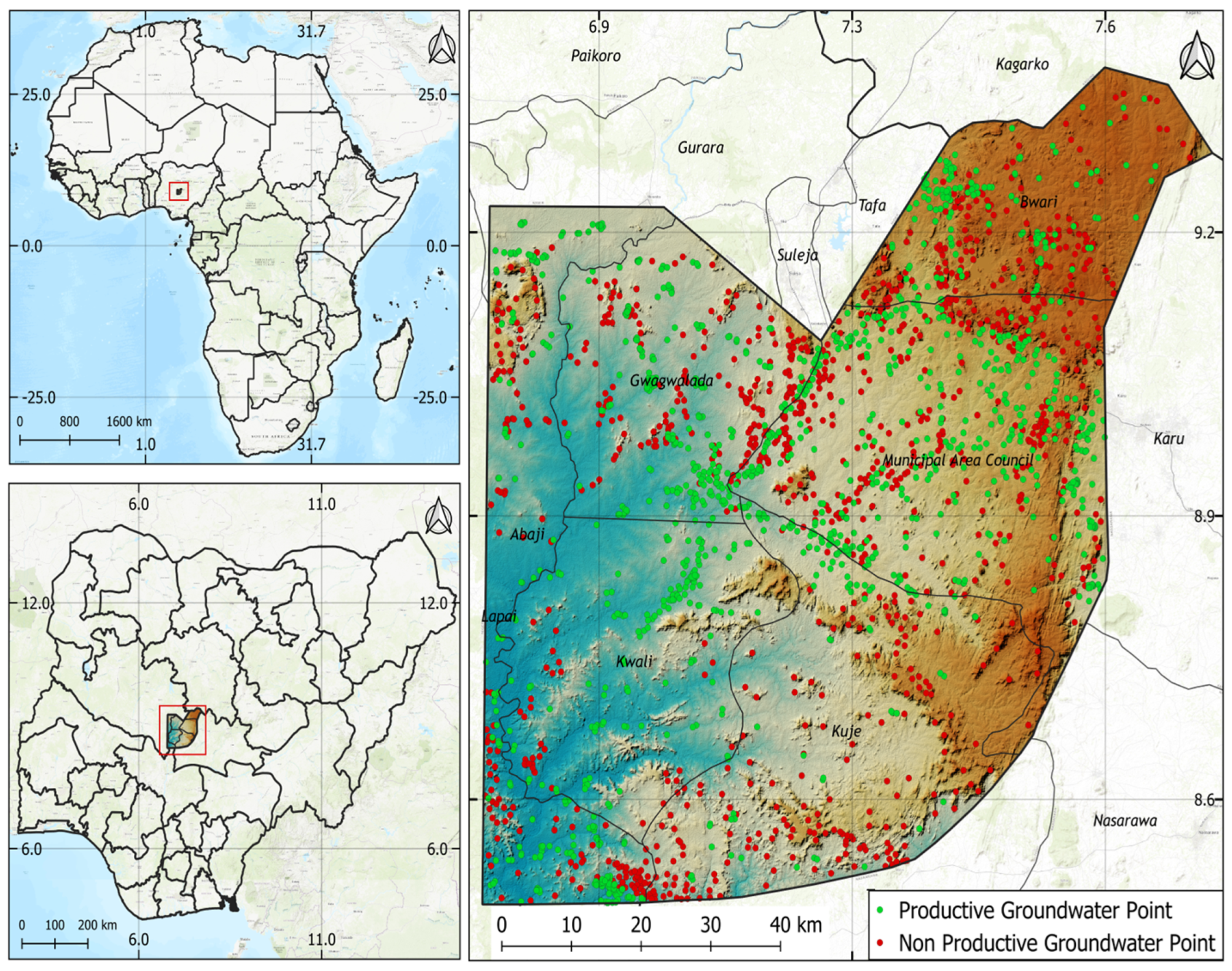
FCT, Abuja is situated between latitudes 8°21′–9°18′ N and longitudes 6°46′–7°37′ E in north-central Nigeria. It has a mean elevation of 476 m above sea level and spans an area of roughly 8000 km² [25] (Figure 1). Urbanisation and rapid population development have put more strain on the city’s groundwater supplies in recent years.

1.2. Geological Settings

Geologically, a large portion of the study area is considered part of the Precambrian basement complex of Nigeria. Crystalline basement rocks account for about 85% of the area, while sedimentary formations constitute around 15%. The dominant structural trends are N–S to NNE–SSW, reflecting deformations generally associated with the Pan-African orogeny, which was formed as a result of the collision between the Pan-African mobile belts and the West African Craton [26].

Rocks in the study region are characterised into four main lithologic units [27]: (i) the migmatite–gneiss complexes, which represent the most dominant rock types; (ii) the metasedimentary belts, including schists, amphibolites, quartzite, phyllites, and serpentinites; (iii) the Older Granite emplaced as concordant to semi-concordant intrusive bodies and (iv) the sedimentary sequence of the Bida Basin, which consist of clay-to-gravel alluvial and shallow marine deposits with thickness ranging from 900 to 2000 m, the outcrops are visible in the southwestern part of the FCT [28]. In addition, unconsolidated alluvial deposits occur along major river channels.

1.3. Hydrogeological Settings of the Study Area

Groundwater occurrence in the study area is generally controlled by two major aquifer systems: (i) the weathered and fractured aquifer (the basement complex), and (ii) the sedimentary aquifer system (Bida Sandstone formation) in the southwestern region. The hydrogeology of the basement complex parts of Abuja matches the typical tropical basement aquifer system of Africa, characterised by weathered regolith overlying fractured crystalline bedrock [29]. Fresh crystalline basement rocks generally lack porosity and permeability but can store and transmit groundwater through secondary porosity and permeability created by the weathering and fracturing. Aquifer productivity, therefore, depends on the thickness of the weathered layer and the degree of structural deformation [29]. The weathered layer encompasses both residual soil and saprolite [29]. Evidence from geophysical exploration and borehole data collected from the study area revealed that the weathered regolith thickness ranges from about 2 m to as deep as 45 m in some places in the basement terrain [30]. The weathered layer is characterised by low to moderate yields and is commonly exploited by locals through hand-pump boreholes and hand-dug wells [31]. The sedimentary formations in the FCT, on the other hand, exhibit relatively higher porosity and permeability and are characterised by moderate to high yield. Aquiferous zones are found in the sedimentary formations at depths ranging from 60 to 120 m [31]. The formation lithologic units are characterised by coarse to fine-grained sandstones, conglomerates, siltstones, and claystones, which are visible in outcrops, particularly around Lokoja. Surrounded by a clay matrix are sub-angular to sub-rounded cobbles, pebbles, and granule-sized quartz grains. Indicating variations in depositional energy, both grain-supported and matrix-supported conglomerates occur at the base of distinct sedimentary cycles [32]. Abuja is characterised by diverse topographical features, with elevation ranging from roughly 76 m in the floodplains along the river Gurara in the southwest to over 760 m in the northeastern uplands of Bwari [31]. Groundwater flow in the region is largely controlled by topography and structural inclinations, and the dominant flow direction is northeast–southwest [31]. Groundwater recharge occurs through infiltration of rainfall and is enhanced in areas of high lineament density, low slope and high permeability, which are controlled by geology [33]. These hydrogeological characteristics control groundwater occurrence in the study area, which influenced the selection of the conditioning factors for this study.

1.4. Climate and Vegetation

The climate of FCT can be described as a tropical continental climate characterised by two distinct seasons: the dry and rainy seasons [34,35]. The area lies in a transition zone between two rainfall-maximum regions to the south and the single rainfall peak in the north, and the average rainfall annually is about 1200 mm/year, occurring between April and October each year [36,37,38]. The weather conditions in the FCT are relatively controlled by the rugged nature of the area, with the hills and inselbergs occasionally inducing orographic (relief) rainfall in their immediate vicinity.

Maximum temperatures under cloudless conditions range from 30 °C in the northeast to 37 °C in the southwest and are experienced during the dry season (November–March). However, during the rainy season (April–October), the temperature drops to approximately 27 °C due to increased cloud cover [39].

Vegetation in the FCT consists mainly of forest and savanna ecosystems. The forest zones dominated by woody plants are divided into rainforest and riparian vegetation complexes, distinguished by species composition and topography. The central and northern parts of the territory are dominated by savanna vegetation, characterised by a mix of trees and grasses [36].

2. Materials and Methods

2.1. Groundwater Potentiality Inventory

Borehole information for this research was compiled from multiple sources, including the FCT Rural Water Supply and Sanitation Agency (FCT-RUWASSA), the Sustainable Development Goals (SDGs) office of the Federal Capital Territory Administration (FCTA) and private borehole-drilling companies operating within Abuja. Included in the dataset are the spatial coordinates of groundwater and non-groundwater points. Groundwater points are represented by productive boreholes (data collected include borehole depth, static water level depth, and water column thickness), while the non-groundwater points are represented by abortive boreholes and rock outcrops. Groundwater in basement terrain is naturally found in fractured rocks or deep weathering zones where infiltration and lateral flow are facilitated by secondary porosity [40,41]. In contrast, exposed, unweathered bedrock outcrops are characterised by low porosity and fractures, which limit infiltration and subsurface storage [42].

Aquifers are generally found between 21 m and 120 m in the FCT’s basement complex terrain, which is consistent with the borehole depth intervals observed in the field [31,42]. Static water levels in the boreholes, which range from 2 to 28 m, indicate the influence of overburden thickness and recharge conditions on the water table in much of the study region.

2.2. Selection and Preparation of Groundwater Conditioning Factors

Groundwater potential (GWP) is controlled by recharge processes, which are themselves governed by a combination of climatic, surface and subsurface factors [43]. The groundwater potential zones of the research region were mapped using nine groundwater-influencing factors. These factors include geology, depth to bedrock, aquifer thickness, slope, lineament density, drainage density, distance from river, land use/land cover (LULC), and rainfall. The thematic layers were generated using information from relevant government agencies and organisations, geophysical investigations and remote sensing data.

The cumulative vertical thickness, measured from the ground surface of unconsolidated and weathered subsurface layers overlying the fresh crystalline basement as determined from the interpretation of vertical electrical sounding (VES) data in this research, is called depth to bedrock (DB). The fresh bedrock horizon is defined as the layer characterised by higher electrical resistivity when compared to the overlying materials, reflecting the transition from weathered or fractured regolith to unweathered and partially fractured basement rocks [44,45]. The thickness and hydraulic properties of the regolith and the fracture density of the underlying basement control groundwater movement and storage in hard rock terrain [29].

Aquifer thickness is the thickness of the saturation zones in a subsurface formation, which indicates the groundwater storage capacity of an area. It was derived from the interpreted VES data obtained through geophysical investigation. The electrical resistivity method, especially VES, is generally recognised as an effective technique for estimating the depth to bedrock, aquifer thickness and the geometry of weathered or fractured zones [44,45]. Two current electrodes (AB) were used to inject an electric current into the subsurface, and two different potential electrodes (MN) were used to assess the potential changes. Subsurface electrical resistivity differences, which are influenced by lithology, fluid content, degree of weathering and fracture, are revealed by variations in the potential field [44]. A Campus Ohmega resistivity meter using the Schlumberger electrode configuration was employed to conduct VES at 823 locations across the study area. During measurement, the maximum half-current electrode spacing (AB/2) was stretched to 100 m, and the maximum potential electrode spacing (MN/2) was kept at 5 metres. Details of this procedure were explained in my previous publication [46]. A partial curve-matching process and computer-aided modelling using IP2Win software (version 3.1.0.a) were used to quantitatively analyse the apparent resistivity data [47]. The depth to bedrock and aquifer thickness were estimated from the interpreted model and then interpolated in QGIS environment to produce the spatial models of the variables across the research region.

Drainage density, lineament density, and slope are known to affect groundwater potential [48,49,50]. The Shuttle Radar Topography Mission (SRTM) Digital Elevation Model (DEM) with 30 m spatial resolution was obtained from the USGS Earth explorer platform (https://earthexplorer.usgs.gov/) on 10 May 2025 and processed in QGIS (version 3.40). The DEM was used to produce the slope, drainage density and lineament density thematic layers, which were subsequently refined through spatial analysis in QGIS. Anthropogenic land-use changes can significantly alter hydrological processes; for this reason, they are widely considered as an important factor in groundwater potential assessment [51]. Employing Google Earth Engine (GEE) platform, the land use/land cover (LULC) map of the research region was produced from 30 m spatial resolution Landsat-8 (OLI) imagery using a supervised classification approach.

In groundwater potential assessment, geology is a crucial factor, as it controls groundwater occurrence, storage capacity and flow dynamics [52]. The geological map of Abuja was extracted from the geological map of Nigeria, produced by the Nigerian Geological Survey Agency (NGSA) (https://www.ngsa.gov.ng) accessed on 10 April 2025 and digitised to produce the geology thematic layer in QGIS (version 3.40). Rainfall is the main source of groundwater recharge, and both surface and subsurface factors that encourage or inhibit infiltration affect how well the recharge process works.

Rainfall data covering a 20-year period were obtained from CHIRPS v2.0 (Climate Hazard Group Infrared Precipitation with Stations) dataset [53] through the climate engine platform (https://climateengine.org) accessed on 5 May 2025. Nigerian Meteorological Agency (NiMet) georeferenced meteorological station records within the study area were used as reference control points for interpolating the CHIRPS data. Station-guided interpolation was performed to create a continuous rainfall distribution map of the study region. An area’s GWP is often increased by having proximity to surface water bodies due to sustained recharge conditions [52,54]. It is often used as a proxy for assessing groundwater recharge potential because it indicates the proximity of each location to surface water bodies in a certain region. The distance-from-river thematic layer was created by using the Euclidean distance function to the digitised drainage network.

Table 1. Groundwater influencing factors, data sources, data type and their hydrogeological relevance.

Hydrogeological Factors	Data Source/Resolution	Data Type	Relevance to Groundwater
Depth to bedrock	Vertical electrical sounding (VES)/(30 m)	Continuous	Determines storage capacity
Aquifer thickness	Vertical electrical sounding (VES)/(30 m)	Continuous	Saturated zone thickness and groundwater storage capacity
Slope	DEM (SRTM)/(30 m)	Continuous	Controls surface runoff, infiltration and flow direction
Geology	Nigeria Geological Survey Agency/(30 m)	Categorical	Influences porosity, permeability.
Lineament density	DEM (SRTM)/(30 m)	Continuous	Indicates fracture zones and zones of high permeability
Drainage density	DEM (SRTM)/(30 m)	Continuous	Inversely related to infiltration
Distance from river	Hydrological datasets (river network)/(30 m)	Continuous	Influences recharge through river/aquifer interaction
Rainfall	CHIRPS/NIMET/(30 m)	Continuous	Primary source of recharge
LULC (land use/land cover)	Sentinel-2 (GEE Classification)/(30 m)	Categorical	Influences infiltration/runoff dynamics

presents the summary of the conditioning factors, including data type, data source, spatial resolution and the relevance of each factor.

2.3. Feature Importance Analysis of Groundwater Conditioning Factors

The relative impact of each conditioning factor on groundwater potential prediction was ascertained using feature importance analysis. Using the built-in impurity-based technique, feature significance for the ensemble-based models (XGBoost and RF) was determined as the average decrease in node impurity among the decision trees. For the SVC model, which generally uses a non-linear RBF Kernel, feature importance was analysed using the permutation_importance function from the scikit-learn library. The importance of each predictor was assessed by randomly shuffling its values and measuring the reduction in model performance. To determine the model’s sensitivity to each feature, the procedure was repeated multiple times.

2.4. Multicollinearity Assessment Method

Multicollinearity develops when two or more predictor variables display overlapping information, which may negatively affect feature importance measures and reduce the classification outcomes [55]. Excessive multicollinearity suggests the presence of redundant predictors that may degrade the classification performance and make the interpretation of results somewhat complicated [55,56]. Therefore, a multicollinearity analysis was carried out before the model development to examine the interdependence among groundwater conditioning factors and ensure model stability. The Pearson correlation coefficient, which measures the degree of linear relationship between predictor variables, was used in this study to assess multicollinearity [57]. Correlation coefficient varies from $-1$ to $+1$, with values close to $\pm 1$ indicating a strong linear relationship and values close to zero demonstrating a weak or negligible relationship. In environmental and geospatial modelling research, significant multicollinearity is defined using a threshold of $\left|r\right|\ge 0.7-0.8$ [58]. To prevent duplication and redundancy, predictors that exhibit high correlation were scrutinised before the modelling.

2.5. Training and Testing Data Preparation

The likelihood that a drilled borehole will yield sufficient groundwater is defined in this research as groundwater potential. Borehole productivity was determined based on yield performance, with productive boreholes characterised as those capable of sustaining a minimum discharge sufficient for hand-pump installation (>0.5 m³/h), as defined by [59]. As a result, the target variable is binary, indicating whether exploitable groundwater is present (productive) or not (non-productive). Productive locations are confirmed productive borehole points, while non-productive locations include abortive or dry boreholes and basement rock outcrops. The combined groundwater and non-groundwater inventory consists of 2410 georeferenced points. The data were randomly split into 80:20 training and testing subsets, with 1928 points for training and 482 points for testing, to minimise bias and take into consideration the varied distribution of the hydrogeological conditions throughout the research region (Figure 2). The GWP models were created using the training dataset; their performances were validated using the testing dataset [60].

2.6. Model Selection and Description

An initial model screening was performed using the “LazyPredict” library within the Python (version 3.12.4) environment to benchmark a wide range of supervised classification algorithms under identical conditions using default hyperparameters [61]. This approach enables comparison of models and was employed in this study for preliminary algorithm selection. A variety of metrics, including overall accuracy, F1 score, balanced accuracy, receiver operating characteristic curve, the area under the curve (ROC-AUC), were used to assess the sampled algorithms performances. Summary results of the model screening are shown in

Table 2. Automated model screening of supervised classifiers for groundwater potential mapping.

S/N0	Algorithm	Accuracy	Balanced Accuracy	F1 Score	ROC–AUC
1	XGBoost Classifier	0.85	0.85	0.85	0.85
2	Random Forest Classifier	0.85	0.85	0.85	0.85
3	LightGBM Classifier	0.84	0.84	0.84	0.84
4	Extra Trees Classifier	0.84	0.84	0.84	0.84
5	Bagging Classifier	0.83	0.83	0.83	0.83
6	K-Nearest Neighbours	0.81	0.81	0.81	0.81
7	Support Vector Classifier	0.81	0.81	0.81	0.81
8	Label Spreading	0.80	0.80	0.80	0.80
9	Label Propagation	0.80	0.80	0.80	0.80
10	Calibrated Classifier (CV)	0.80	0.80	0.80	0.80
11	Logistic Regression	0.80	0.80	0.80	0.80
12	Linear SVC	0.80	0.80	0.80	0.80
13	SGD Classifier	0.79	0.79	0.79	0.79
14	AdaBoost Classifier	0.79	0.79	0.79	0.79

, which shows that ensemble-based tree models attained the highest predictive performance. SVM also performs competitively, ranking it among the top non-ensemble classifiers. Three ML algorithms: XGBoost, Random Forest (RF) and Support Vector Machine were chosen from the screened algorithms for the GWPZ mapping in this research, and their strength and capabilities are discussed as follows.

2.6.1. Extreme Gradient Boosting (XGBoost) Algorithm

XGBoost originally proposed by [62], is a cutting-edge ensemble learning method created to achieve excellent computational efficiency and accuracy for classification and regression issues. The algorithm execution speed, scalability and generalisation have made it prominent in geospatial and environmental studies [63]. XGBoost creates a learner by progressively combining several weak learners, typically regression trees, within an additive boosting framework to lower prediction error. Every new tree is trained to simulate the prior ensemble residuals [64].

The forecast for a specified sample is derived by adding together each tree’s contributions within the ensemble:

$${\hat{y}}_i={\displaystyle \sum _{t=1}^T}{f}_t\left(x_i\right)$$

(1)

where $f_t$ is the decision tree added at iteration t, $x_i$ represents the input feature vector, and T is the total number of trees [63].

Model training is controlled by a regularised objective function that balances the integrity of fit with model complexity and is commonly expressed as follows:

$$L^{\left(t\right)}={\displaystyle \sum _{i=1}^n}l\left(y_i,{{\hat{y}}_i}^{(t-1)}+f_t\left(x_i\right)\right)+\mathsf{\Omega }\left(f_t\right)$$

(2)

where $l$ is a differentiable loss function and $\mathsf{\Omega }\left(f_t\right)$ is a regularisation term that penalises overly complex trees to mitigate overfitting [62,65]. Internal cross-validation, shrinkage, and column subsampling are incorporated into XGBoost to improve the efficiency of the model [66,67]. These features enable the algorithm to carry out accurate predictions with very little overfitting and make it suited for complex nonlinear modelling tasks, including groundwater potential modelling [63,68].

2.6.2. Random Forest (RF) Algorithm

RF is an ensemble learning technique that groups predictions of multiple trained decision trees, thereby enhancing generalisation and accuracy [69,70]. In RF, each decision tree is constructed by employing bootstrap sampling from the original dataset, while randomness is further introduced by selecting a subset of predictor variables at each node to determine the split, which reduces inter-tree correlation and moderates overfitting without the need for post-lopping [69,71,72]. The final model output is obtained through majority voting across all trees for a classification task while for regression problems it is computed as the average of individual tree predictions [73]. A distinguishing feature of RF is the inclusion of out-of-bag (OOB) samples, which are roughly one-third of the data not included in the bootstrap sample for a given tree, and provide an internal and objective evaluation of model performance and generalisation error [69,70]. The mean squared error (MSE) is used to quantify the OOB error between observed and predicted values for the OOB samples, expressed as

$$E_{OOB}={\displaystyle \frac{1}{n}}{\displaystyle \sum _{i=1}^n}{(y_i-{\hat{y}}_i)}^2$$

(3)

where n is the number of out-of-bag observations,${ y}_i$ denotes the observed response, and ${\hat{y}}_i$ is the corresponding RF prediction [74,75]. Random Forest technique is used for geospatial and environmental modelling tasks due to its ensemble-based architecture, which balances bias and variance, and its resilience to noise and nonlinear interactions [73,75].

2.6.3. Support Vector Machine (SVM)

SVM is a supervised machine learning method that has been widely utilised for regression and classification problems in groundwater and environmental research. It is rooted in statistical learning theory and the concept of risk minimisation [8,76,77]. SVM is frequently used in groundwater potential study as Support Vector Classification (SVC), which assigns a discrete groundwater potential zone (GWPZ) based on pertinent groundwater influencing parameters or Support Vector Regression (SVR), which generates continuous prediction [23,78]. The objective of this modelling technique (SVM) is to identify an optimal separating hyperplane that maximises the margin between data points of different classes within a high-dimensional feature space, thus improving generalisation capability [79,80]. Equation (4) defines the decision function for linearly separable data.

$$f\left(x\right)=w^{T}x+b,$$

(4)

where x is the input feature vector, $w^T$ is the transpose of the weight vector controlling the orientation of the hyperplane, and b is the bias term [81]. To address nonlinearly separable cases, SVM introduces a regularised optimisation framework that balances margin maximisation and classification error using the hinge loss function, as shown in Equation (5).

$$min{\displaystyle \frac{1}{2}}{\parallel w\parallel }^2+C{\displaystyle \sum _{i=1}^n}max\left(\mathrm{0,1}-y_{i }\left(w^T{x}_i+b\right)\right),$$

(5)

where $y_{i }$ is the class label, C is the penalty parameter controlling the trade-off between margin width and misclassification, and the loss term penalises margin violation [82]. By implicitly mapping input data into higher-dimensional spaces, the kernel function improves SVM performance. This allows for the modelling of intricate nonlinear interactions, and prediction accuracy depends upon proper kernel selection and parameter tweaking [83]. Support Vector Classifier (SVC), a subset of SVM, has proven to be a reliable technique for mapping GWPZ in complex hydrogeological settings due to its predictive accuracy, resistance to overfitting and computational complexity that is essentially independent of dimensionality input [23,77]. It develops an optimal hyperplane that enables modelling of nonlinear relationships between groundwater occurrence and controlling factors by maximising the boundary between classes in a high-dimensional feature space [84,85]. Although kernel and hyperparameter modification affects its prediction accuracy, for groundwater studies with small training data, SVC is appropriate [86,87].

2.7. Groundwater Potential Modelling Framework

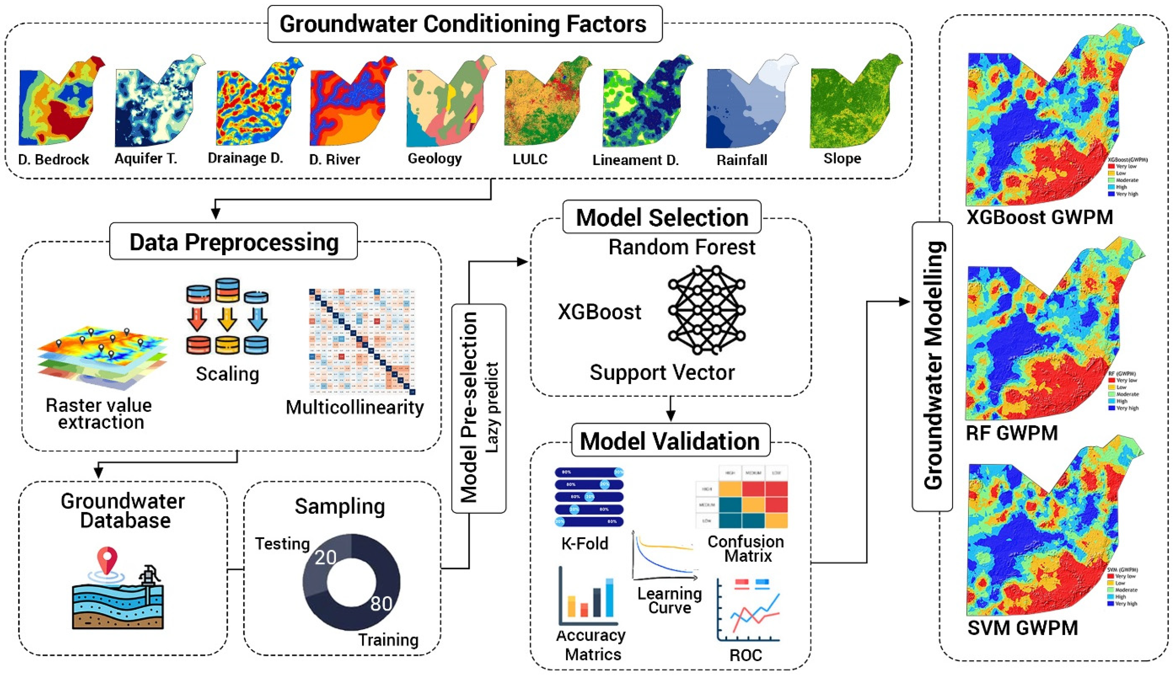
GWPZ maps were created following the workflow that integrates geospatial analysis and ML techniques, as shown in Figure 2. To ensure consistency in the analysis, groundwater conditioning factors for this research were prepared as raster layers using uniform spatial resolution and projection. Aquifer thickness, depth to bedrock, slope, drainage density, rainfall and lineament density are continuous variables and were left in their original form and before being normalised to lessen scale effects. Categorical variables such as geology and land use/land cover (LULC) were transformed using one-hot encoding technique. Multicollinearity among the influencing factors was evaluated using the Pearson correlation analysis to establish the independence of the input variables.

The predictor dataset used to develop the machine learning model was created by overlaying groundwater inventory data that included borehole locations (presence and absence points) on the thematic layers and extracting corresponding pixel values for each conditioning factor. A binary variable was assigned to each borehole point; productive boreholes were classified as presence (1) while abortive boreholes were classified as absence (0). A structured dataset comprising predictor and target variables was generated and subsequently partitioned randomly into training (80%) and testing subsets (20%) to develop and validate the models.

The ML models (XGBoost, RF and SVM) were trained using the conditioning factors as predictors; the trained models were then applied to the entire set of predictors to generate continuous probability values, which represent the groundwater potential across the FCT. The probability values (predicted point) were interpolated in QGIS to produce a continuous GWP map, which was subsequently reclassified into five classes: very high, high, moderate, low, and very low potentials. The model was finally validated using independent test data to assess the comparative model performance and accuracy.

2.8. Validation and Performance Assessments of the Models

Model validation is one of the critical components of predictive modelling, because it ensures scientific reliability of the generated outcomes [22,88]. The ROC and AUC were adopted as the primary validation metrics in this study to assess the performance of the models in distinguishing between the occurrence and non-occurrence of groundwater potential. It is a generally accepted diagnostic tool for assessing the discriminatory capability of classification models [71,89]. The ROC curve is produced by plotting sensitivity (TPR) against the 1-Specificity (FPR) across a range of decision thresholds [90]. ROC-AUC value varies from zero (0) to one (1), where values closer to 1 suggest higher model performance accuracy; values near 0.5, on the other hand, reflect random predictions [22,71,88]. The choice of ROC-AUC as the primary metric in this research is justified by its suitability for binary classification in research such as groundwater potential modelling [91].

The model’s performance was evaluated using an integration of stratified k-fold cross-validation, hold-out validation and learning curve analysis. Using a hold-out validation method, the dataset was split into 80% and 20%, which represent training and testing datasets, respectively [92,93]. Hold-out validation, which divides the dataset into two subsets (training and testing sets), is a common resampling technique for model evaluation. The testing data are not used during model training, which prevents biased assessments of model performance [92,93].

Stratified k-fold cross-validation (k = 10) was used to minimise variations commonly associated with a single data split. The dataset was split into 10 subsets; each of which was used once for validation, and the remaining folds were used for training. The final estimate was obtained by averaging the validation results across the folds [92,94]. Unlike the standard k-fold approach, the stratified approach ensures that each fold retains the same fraction of productive and non-productive groundwater sites as the original dataset.

Confusion matrix analysis was used in addition to the ROC-AUC to evaluate the classification performance, yielding additional metrics such as accuracy, precision, recall, and F1 score. The F1 score, which represents the harmonic mean (precision and recall), suggests the trade-off between false positives and false negatives; accuracy, on the other hand, offers a general overview [95].

Cross-validation was used in the learning curve analysis to assess how the model behaved in relation to the size of the training sample. This method is used to determine if a model is overfitting or underfitting and to assess its stability when the amount of data increases [93,96]. Each of these validation techniques was used to improve the GWP model’s dependability.

3. Results and Model Evaluation

GIS-based machine learning methods were used to map Abuja GWPZs. Nine groundwater-influencing variables that control groundwater availability in the study area were used: geology, depth to bedrock, aquifer thickness, slope, lineament density, drainage density, LULC, rainfall and distance from river. The mapping was carried out in the study area using RF, SVM and XGBoost classification techniques. To train and assess the machine learning algorithms, 2410 georeferenced groundwater sites in the area, both productive and non-productive, were selected at random. These arbitrary sites were used by the trained algorithms to predict the GWPZ map.

3.1. Spatial Analysis of Groundwater Conditioning Factors

3.1.1. Geology

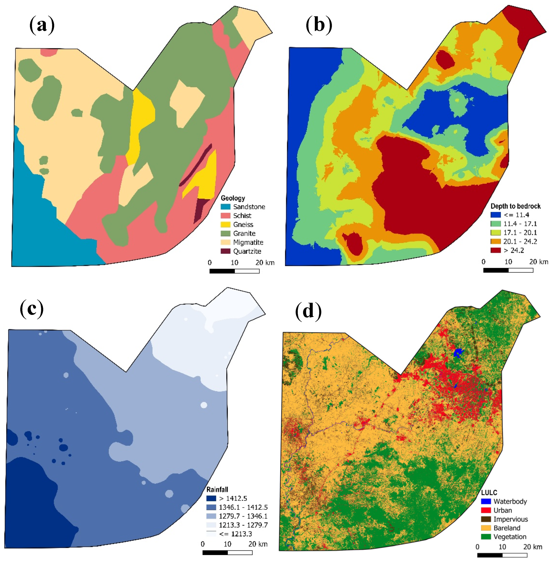
Precambrian crystalline basement rocks make up 85% of the FCT, with sedimentary terrain making up the remaining 15% (Figure 3a). The distribution of the mapped lithology indicates a crystalline framework that is structurally controlled and intruded by granitic bodies and locally overlain by sedimentary formations, which agrees with the geological setting of north-central Nigeria. The basement complex comprises of migmatitic gneiss, biotite–hornblende gneiss, muscovite schists, quartzite, and undifferentiated schists including phyllites. These lithologies were produced during the Pan-African orogeny, which subjects the Nigerian basement complex to structural changes characterised by foliation, joints, faults and shear zones [97,98]. Granitic intrusions are widespread and include coarse porphyritic biotite and biotite-hornblende granites as well as undifferentiated granites, migmatites and granite gneiss complex. Distributed across the central and northern sectors of the territory, granitic rocks occur as discrete plutonic bodies. Their irregular form implies that they were formed during the pan-African Orogeny’s late to post-tectonic phase [97,98]. The crystalline basement rocks in the study area exhibit negligible primary porosity; however, groundwater occurrence is enhanced by secondary porosity and permeability developed through weathering and tectonic fracturing [99].

The sedimentary component of the FCT, represented by feldspathic sandstone and siltstone, occurs mainly in the southwestern margin of the territory and corresponds to the Lokoja Formation of the Bida Basin. They are characterised by relatively higher primary porosity and permeability, which makes them more promising in groundwater potential when compared to the crystalline basement [100]. Lithology controls the occurrence and movement of groundwater in the Abuja, with higher groundwater potential commonly associated with sedimentary formations and highly weathered or fractured basement terrains [31].

3.1.2. Depth to Bedrock (DB)

The research area’s depth-to-bedrock map (Figure 3b) shows a DB range of less than 11 m to more than 24 m; structural and geomorphological reasons may be responsible for this. Shallow depths (<11 m) are mainly found along the western margin and in a few locations in the region’s centre. These regions are distinguished by thin regolith layers, sporadic rock outcrops and limited weathering. Transitional belts are characterised by moderate depths (11 m–20 m), which correspond to areas of high weathering or fracturing in hard rock. Broad depressions weathered or structurally controlled zones of weakness and the deepest bedrock surfaces (>20 m) are found in the southwestern and southeastern portions of the research region. In basement terrain, these depressions are associated with fracture networks, shear zones or contact zones that promote weathering and high regolith thickness, particularly in tropical climates [29,101].

Groundwater occurrence and movement are often controlled by the distribution pattern of DB. Where regolith coincides with the underlying fractured rock, favourable conditions (storage and transmission) are created for a productive aquifer [44,101]. The DB configuration in the study area reflects a common characteristic of the typical Nigerian basement complex aquifer, in which secondary porosity is produced by the combined effects of lithology, weathering and tectonic activities.

3.1.3. Rainfall

The average annual rainfall across the study area (Figure 3c) decreases as you move from the southwestern part of the study area to the northeastern part and ranges from over 1412 mm to less than 1213 mm annually. The southwestern region and certain areas of the southern region receive the most rainfall. The northeastern portion of the region has comparatively lower rainfall figures. The West African Monsoon System regulates the rainfall patterns. Humid south-westerly air masses from the Atlantic Ocean gradually lose their moisture as they travel inland, creating a south–north gradient of rainfall across most parts of central Nigeria [102,103]. Orographic influences and interaction between the surface and the atmosphere, which are caused by the variation in relief across the study area, could also be responsible for the rainfall gradient.

The research region’s GWP is significantly influenced by rainfall, which is the primary source of groundwater recharge, particularly in a crystalline basement environment where recharge is sporadic. Variation in rainfall within the region also has an impact on groundwater availability [104,105]. Regions with higher annual rainfall in the southwestern parts of the FCT are thus expected to exhibit higher recharge potential, provided the slope, soil permeability and regolith thickness are favourable for infiltration. On the other hand, areas with little rainfall, particularly the northeastern part of the study area, may have lower groundwater potential.

3.1.4. Land Use/Land Cover (LULC)

An area’s LULC pattern affects groundwater recharge processes, which makes it crucial for defining groundwater potential zones [106,107]. Because the LULC pattern regulates the surface runoff and infiltration rate, an area’s groundwater potentiality could rise or fall depending on the pattern. The 2023 LULC map of Abuja (Figure 3d) reveals various land-use patterns in the study area, including bare surfaces, water bodies, impervious surfaces, urban and vegetation (cultivated land, forest and woodland). The map depicts a terrain where bare surface and vegetation dominate. The majority of the southern and southeastern regions are covered by vegetation, which reflects an agricultural landscape and natural land cover. The central and northeastern parts of the region have a concentration of urban and impervious surfaces. Although they make up a small percentage of the territory, water bodies like rivers and reservoirs are crucial to the development of the groundwater aquifer.

Urban and impervious areas reduce infiltration and increase surface runoff due to their water-resistant nature, which limits groundwater recharge and alters the hydrological cycle [108]. Vegetation cover, on the other hand, decreases runoff velocity, enhances infiltration and promotes soil moisture retention, which supports groundwater recharge processes under favourable conditions such as regolith thickness and permeability [109]. The LULC pattern of the FCT, as shown in the LULC map, has direct implications for groundwater potential modelling in the area, which makes its integration with other groundwater influencing factors essential.

3.1.5. Slope

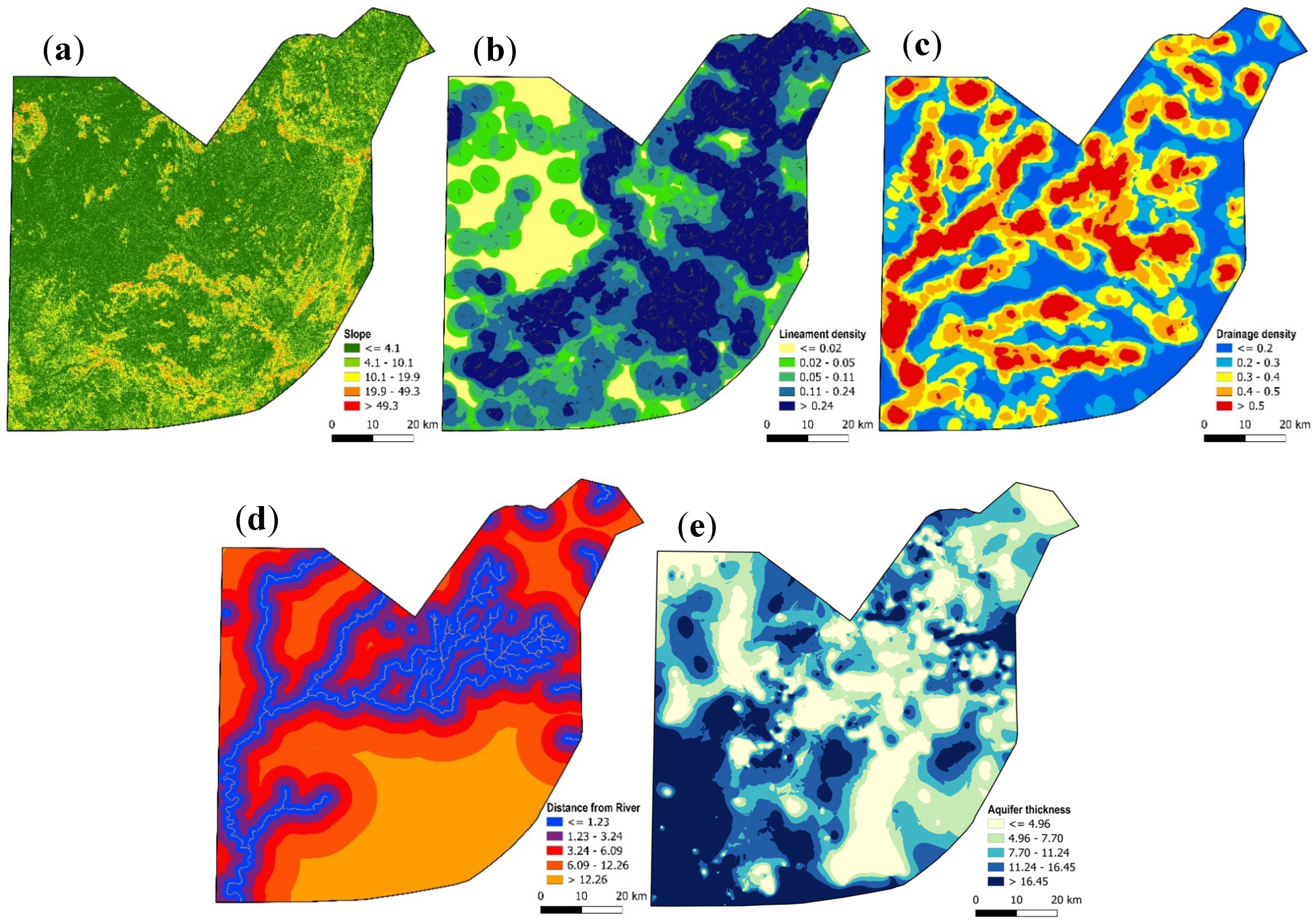
The slope map of the study area (Figure 4a) displays an area that mainly consists of low gradient surfaces with slope values in most areas ranging from 0° to 10.10°, which indicates gently rolling plains of weathered Precambrian basement formations. The gentle slopes occupy the central and western regions of the study area; rocks in such areas are characterised by tropical weathering processes [101,110]. Moderate slopes (10.10° and 49.30°) appear as scattered bands, while steep slopes (over 49.30°) are found mostly in the southern and southeastern areas; they are typically residual hills and ridges of resistant rock types such as quartzite and granites. Slopes are known to play an important role in determining surface runoff, infiltration, erosion, and groundwater recharge. Gentle slopes encourage infiltration and groundwater recharge by slowing runoff; steep slopes on the other hand facilitate rapid surface flow, which limits effective recharge [111,112].

3.1.6. Lineament Density

Lineaments are products of structural and tectonic processes that often appear as linear or curvilinear structures [113]. They reflect the subsurface geological structure of an area and are commonly described as faults, joints and fractures [114]. They are generally found in crystalline basement terrains and serve as the secondary porosity that encourages infiltration and stores and transmits groundwater [115]. Because they serve as proxies for groundwater availability, particularly in hard rock terrain, lineaments are regarded as one of the most significant structural elements when it comes to groundwater potential delineation.

Five classifications of lineaments are shown in the research area’s lineament density map (Figure 4b): very high (>0.24 km²), high (0.11–0.24 km²), medium (0.05–0.11 km²), low (0.02–0.05 km²) and very low (≤0.02 km²). High lineament density dominates the central, southeastern and northeastern parts of the region, and lower densities were observed in the western and northwestern areas. The distribution and structural pattern of the lineaments could be linked to the Pan-Orogeny that affects the Nigerian basement complex [97,98]. Areas with higher lineament density are interpreted as having greater structural permeability, which promotes groundwater recharge, storage and transmissivity, especially at the junctions of fractures and weathered regolith, and vice versa.

3.1.7. Drainage Density

The total length of streams per unit area is defined as the drainage density. It plays a critical role in the distribution of runoff and infiltration rates, making it a vital indicator of groundwater potential [116]. Minimal drainage density often encourages infiltration due to low runoff and contributes to groundwater recharge. In contrast, high drainage density generally inhibits infiltration due to high runoff [117,118].

Drainage pattern is defined by surface and subsurface formations such as lithology, soil permeability, slope gradient and climatic conditions [119]. The drainage pattern in the study area can be described as dendritic (Figure 4c). The research region was classified into five classes and characterised as very high (>0.5 km⁄km²), high (0.4–0.5 km⁄km²), moderate (0.3–0.4 km⁄km²), low (0.2–0.3 km⁄km²) and very low (≤0.2 km⁄km²). High drainage densities are observed across the central and southwestern parts of the region and some portions of the northeastern area. They form an elongated dendritic pattern that indicates the structural influence of the fractured basement terrain. Very low and low drainage densities are randomly distributed across the study area, though they seem more pronounced in some areas than others.

3.1.8. Distance from River

Proximity to stream influences groundwater recharge and serves as an important indicator for groundwater occurrence and development of shallow aquifers [29,101]. Proximity to stream map of the FCT (Figure 4d) shows that the Euclidean distance between the drainage system in the area varies from roughly less than 1.23 km in zones close to the river channels to over 12.26 km for zones far away from the river network. Areas with minimal proximity to the stream are found around the dendritic drainage network that criss-crosses the central and northern parts of the region. The southern and southeastern parts of the region display a relatively larger distance from the major river network. Interactions between surface and groundwater systems are at their best in areas close to the stream, especially in areas where alluvial deposits overlay fracture bedrocks and provide transmissive pathways [120,121].

3.1.9. Aquifer Thickness

The distribution of aquifer thickness (Figure 4e) revealed the heterogeneous characteristics of the research area. Aquifers are crucial factors in determining the occurrence of groundwater because they store and transmit groundwater. The research area’s aquifer thickness ranges from ≤4.6 m to >16.45 m, and was categorised into five classes: very high, high, moderate, low and very low thickness zones. Very high aquifer thickness (>16.45) dominates the southwestern and portion of the central-western areas shown by dark blue. This zone corresponds to the sedimentary parts and regions with a highly weathered profile in the FCT. High overburden thicknesses in the hard rock parts of Abuja are generally linked to tectonic fracturing and chemical weathering, both of which encourage groundwater accumulation.

Moderate to low thickness zones (4.96–11.24 m) are observed in the central and northeastern areas, which reflect moderately weathered bedrock often characterised by limited storage capacity. The very low thickness zones (≤4.96 m) are observed in parts of the central and northeastern region, reflecting shallow overburden thickness, and are generally unfavourable for groundwater development. The spatial pattern of the aquifer thickness is consistent with groundwater occurrence in hard rock terrains, where productivity is governed by the thickness of the weathered layer and structural features [29,101].

3.2. Results of Multicollinearity Assessment

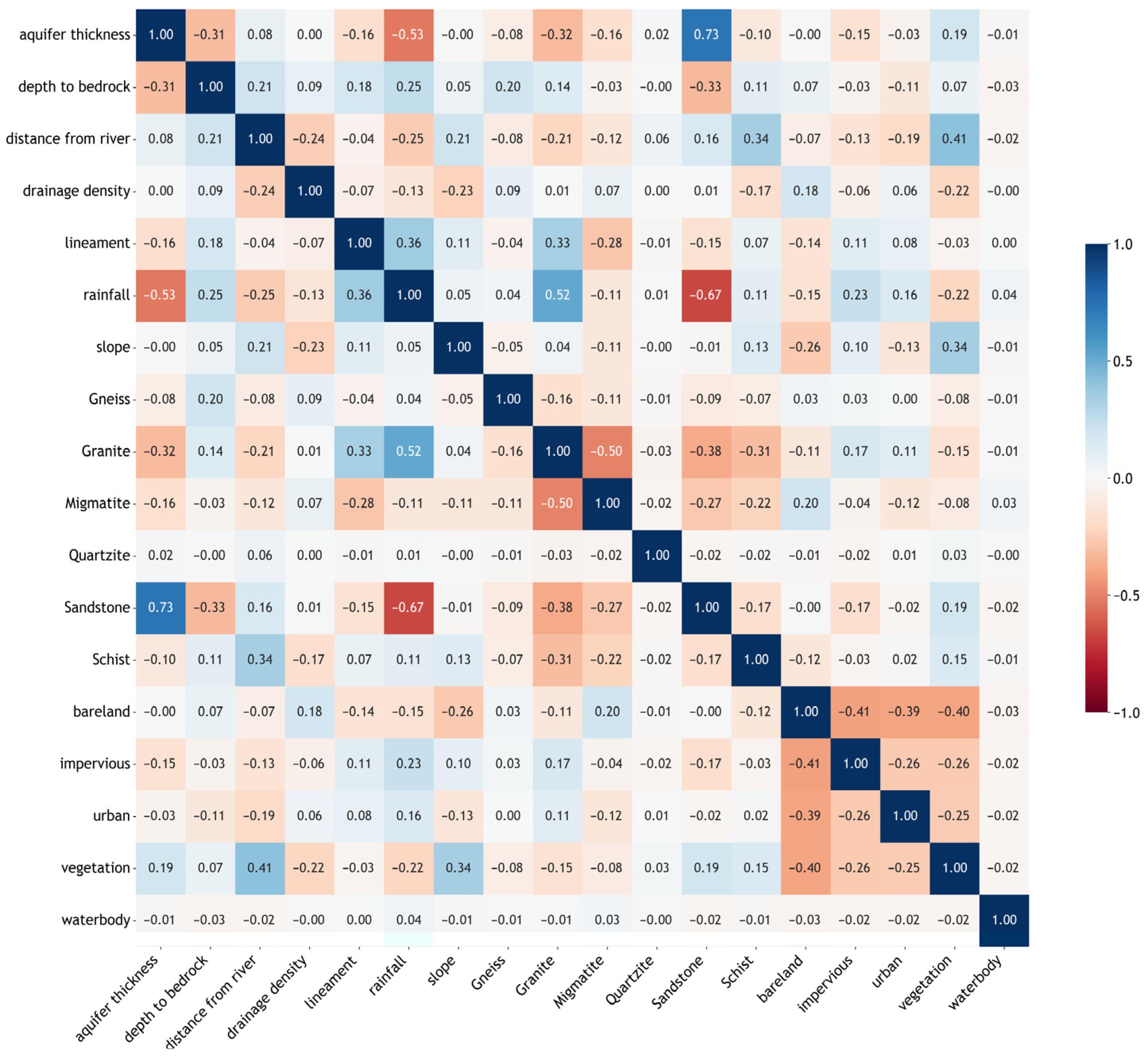
Figure 5 shows the assessment of multicollinearity among the predictor variables using a Pearson correlation described in Section 2.4. The pairwise correlation coefficients are represented as colour grades, with values ranging from +1.0 (strong positive in dark blue) to −1.0 (strong negative in dark red). Coefficients that are close to zero (0) indicate low or insignificant relationships. There is no defined scale, but earlier studies have reported correlation limits that range from 0.40 to 0.85, which are considered acceptable depending on the aim of the modelling and data structure [122,123,124].

The correlation matrix (Figure 5) indicates mainly low to moderate correlations among the variables, confirming the absence of reasonable multicollinearity, which suggests that the selected groundwater conditioning factors are mostly independent, justifying their inclusion in the modelling framework. Most of the correlation coefficient remains below the generally cited thresholds (|r| ≥ 0.7–0.8), which also indicates the lack of any major multicollinearity [122,125]. Strong positive correlations were observed between aquifer thickness and sandstone (r ≈ 0.73), which reflect lithological control on the aquifer development, especially within the sedimentary units. Moderate positive correlations were observed between rainfall and granite (r ≈ 0.52), followed by distance from river and vegetation (r ≈ 0.41), and then lineament density and rainfall (r ≈ 0.36). This correlation indicates the relationship between the lithology and the hydro-environment. Strong negative correlation is observed between rainfall and sandstone (r ≈ −0.67), which suggests spatial patterns that are contrasting between precipitation and sedimentary formation in the study area. Moderate negative correlations were observed among land-use/land-cover classes, which was expected because of their mutually exclusive nature rather than statistical redundancy. Important hydrogeological predictors, including depth to bedrock, lineament density, slope, rainfall, drainage density, distance from river and lithological units, show weak intercorrelations, which implies that each variable contributes complementary information to the groundwater occurrence modelling. Other key hydrogeological variables: slope, depth to bedrock, drainage density and lineament density exhibit weak intercorrelations, indicating that each factor contributes complementary information to the modelling process.

3.3. Feature Importance Analysis

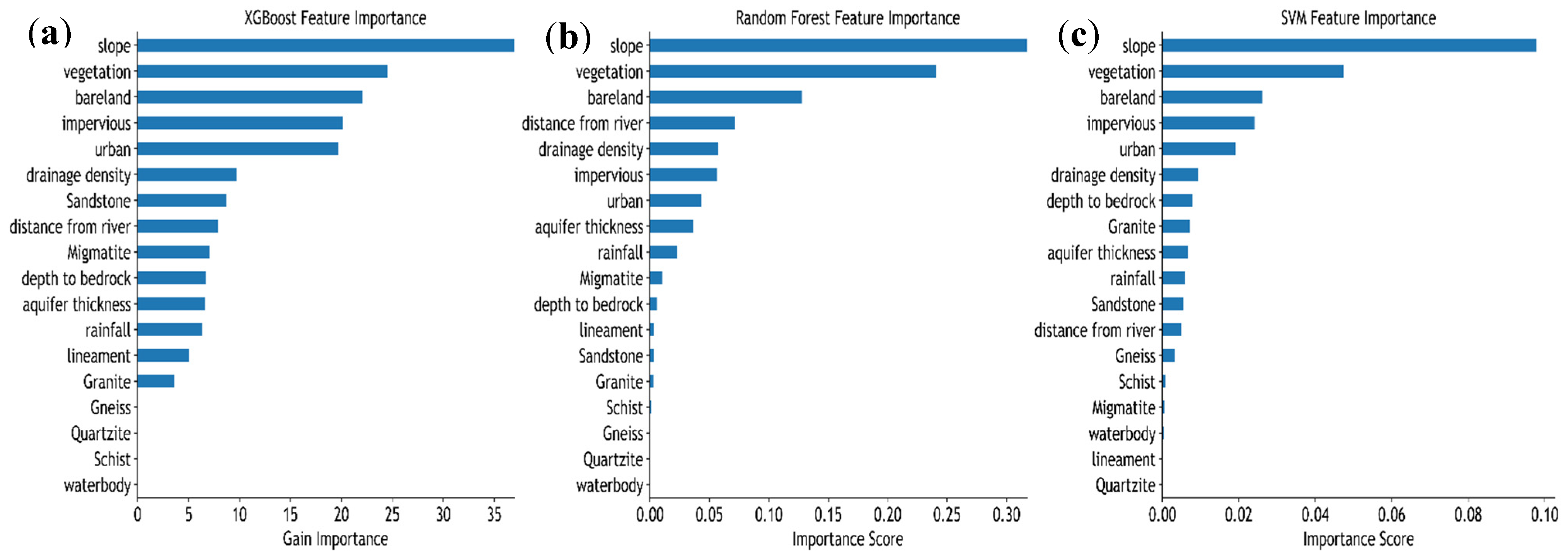
Assessing the reliability and significance of groundwater conditioning factors is crucial before the modelling process commences. Eighteen (18) predictor variables used in this research were evaluated to determine their feature importance as shown in Figure 6. Embedded importance metrics were used for the ensemble tree-based models (XGBoost and Random Forest). Among all the conditioning factors, slope appears to be the most significant predictor across all the models. The results agree with hydrological principles, because terrain gradients are known to influence runoff and infiltration, which often support or inhibit groundwater recharge [111,112]. In the XGBoost model, vegetation, bare land, urban areas and impervious surface appear to be the most dominant factors after slope, which highlights the role of LULC pattern on groundwater recharge of the region. Vegetation increases infiltration rate while impervious surfaces increase runoff and reduce infiltration, both of which influence the groundwater potential of an area [106,107]. Variables like distance from river, drainage density as well as aquifer thickness and depth to bedrock exhibit a moderate contribution, which indicates their role in groundwater occurrence in the area.

For the Random Forest model, there exists a pattern similar to the XGBoost, with slope and vegetation dominating, followed by distance from river and drainage density. Unlike the XGBoost, hydro-geomorphological factors (drainage density and distance from river) indicate high influence on groundwater potentiality of the area, which could be attributed to its sensitivity to drainage characteristics and their effect on storage capability. Aquifer thickness and rainfall also show moderate influence, indicating the role of precipitation and regolith thickness in aquifer development in the area [104,105].

A more simplified importance structure is observed in the SVM model, where slope and LULC-related classes show a dominant influence, while other predictors show marginal influence (Figure 6c), which showcases the limitation of the SVM model in this research and may be responsible for its relatively lower predictive accuracy. Lithological variables such as granite, gneiss, schist, migmatite and quartzite exhibit moderate to low importance across all the models. Although lithology type plays an important role in determining weathering profile, fracture density and secondary porosity development, especially in hard rock terrain, its relatively low ranking suggests that surface and subsurface factors exert greater influence on groundwater occurrence in the area. The feature importance analysis generally demonstrates that topography and land surface conditions have more influence on the groundwater potential of the area, with the subsurface factors playing a complementary role.

3.4. Model Performance Evaluation Results

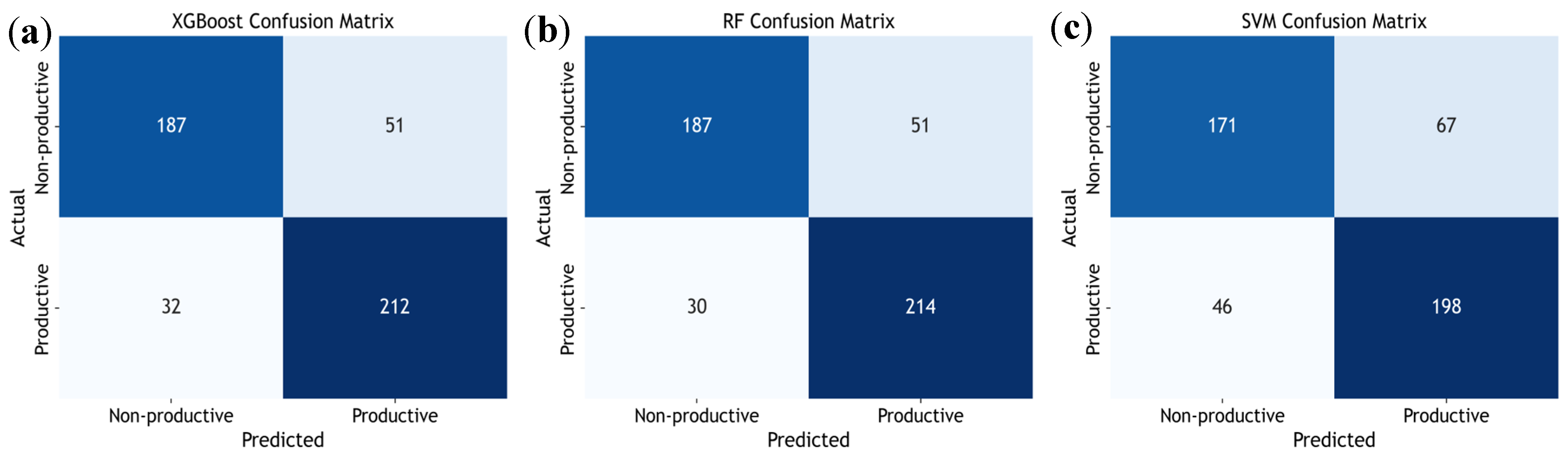
The performance of the three models utilised in this work was assessed using a test dataset (n = 482), comprising 238 non-productive and 244 productive boreholes, the near-equal class distribution was to minimise accuracy inflation due to class dominance. Evaluation metrics used include overall accuracy, precision, F1 score, recall (sensitivity) and confusion matrix analysis for each classifier (Figure 7).

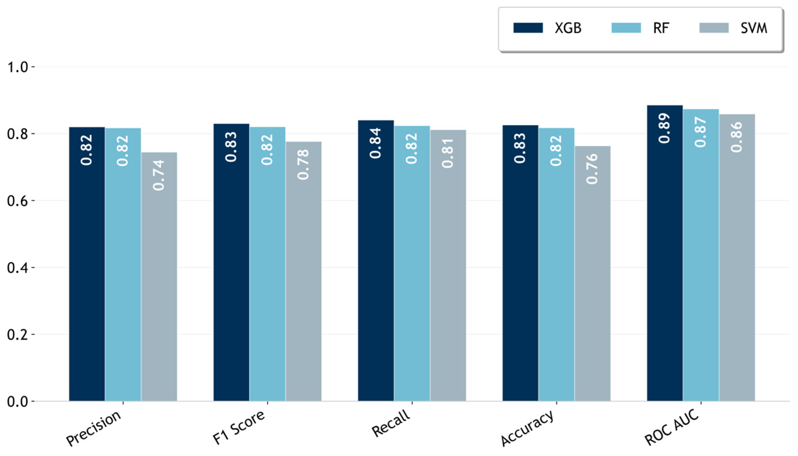
The findings show that Random Forest and XGBoost have superior accuracy. Overall accuracy is highest with RF (0.832), followed by XGBoost (0.828). Conversely, with an overall accuracy of 0.765, the SVM performs relatively lower. The XGBoost model accurately classified 212 productive and 187 non-productive boreholes. It displayed a relatively low misclassification rate, with false positive (FP) = 51; false negative (FN) = 32, as shown in Figure 7a and a balanced precision and recall across both classes (≈0.81–0.88) with an F1 score of 0.84, which indicates a balanced trade-off between omission and commission errors. Random Forest also correctly identified 187 non-productive and 214 productive occurrences, with 51 FP and 30 FN. The model displayed stable and balanced performance, which demonstrates its generalisation ability (Figure 7b). Although the two models (XGBoost and RF) display marginal differences in accuracy (<0.5%), both models display better performance compared to SVM.

In contrast, SVM showed relatively weaker performance; it classified correctly 198 productive occurrences and misclassified a reasonable number of non-productive occurrences (FP = 67) and displayed a higher number of false negatives (FN = 46) (Figure 7c). A higher false positive rate often indicates the tendency to overpredict the positive class, which could lead to overestimation of GWPZ. The model, however, achieved an accuracy of 0.765, a precision of roughly 0.75, a recall of 0.81 and an F1 score of 0.78. The high misclassification rates and relatively lower F1 score (~0.78) suggest that the SVM struggles to capture the complex nonlinear relationship among the input features.

In groundwater potential prediction, it is important to minimise false negatives to prevent exclusion of feasible groundwater targets. When compared to the SVM, both XGBoost and RF display fewer false negatives, which makes their prediction of GWPZ more reliable. The better performance of XGBoost and RF models could be attributed to their capacity to model nonlinearity and hierarchical relationships among features. Figure 8 shows the comparative performance metrics of the three models.

3.5. Spatial Distribution of Groundwater Potential Zones

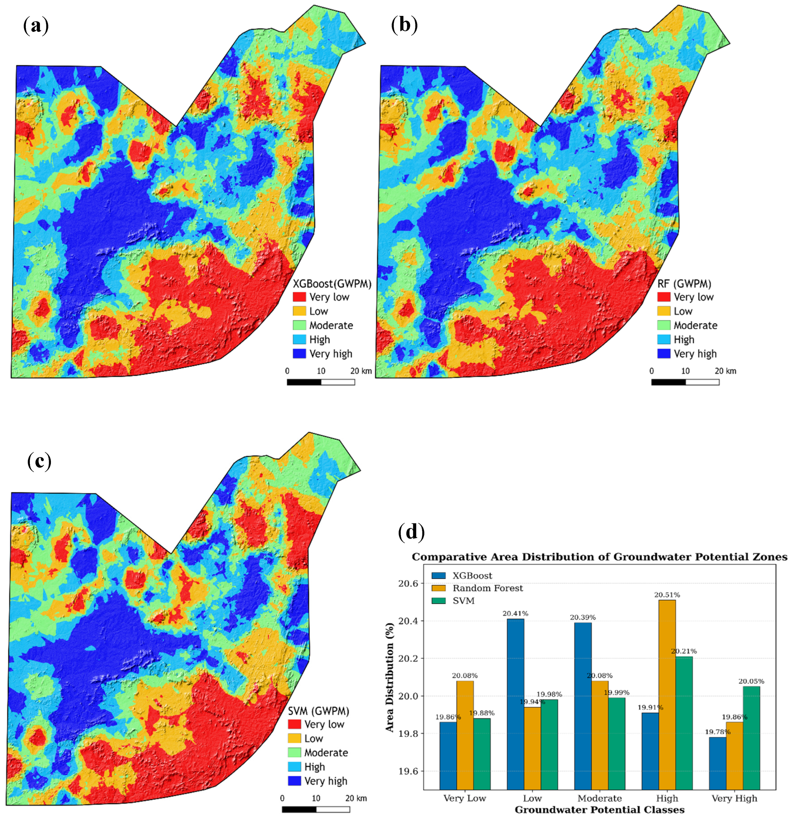
Groundwater potential zone maps were created using three GIS-based machine learning algorithms: XGBoost, RF and SVM. The predicted GWPZ maps were reclassified into five different classes: very low, low, moderate, high and very high using the quantile classification method. Figure 9 illustrates the spatial differences of the GWPZ and the area proportions for each classification as predicted by the three models.

The XGBoost model displays a groundwater potential landscape, with very high and high potential zones situated in the southwestern and northwestern regions, parts of the central area and some patches in the eastern part of the study area (Figure 9a). These areas are relatively flat, which favours groundwater recharge through infiltration. Sandwiched between the lower-yield zones in the northeastern part and the very high potential zone in the southwestern part is a portion of the central region characterised by diverse potential classes, though dominated by the moderate class. Very low and low potential zones, on the other hand, dominate the southeastern parts of the FCT and are characterised by elevated and rugged terrain. Graphically, the XGBoost model exhibits roughly equal distribution across the various classes: very high (19.78%), high (19.91%), moderate (20.39%), low (20.41%) and very low (19.86%), as illustrated in Figure 9d.

The Random Forest (RF) model displays similar distribution pattern to that of the XGBoost, with very high and high potential zones dominating the western and southwestern parts of the FCT (Figure 9b). Moderate potential zones are commonly distributed around the central area. As with the XGBoost model, the very low potential zones are pronounced in the southeastern parts and some sporadic distribution in other parts of the study area. In terms of area distribution, when compared to the XGBoost, the RF model exhibits a slightly different distribution trend. The high potential zone class have the highest area coverage (20.51%), followed by the moderate (20.08%) and very low zones (20.08%), which share the same area coverage. Low (19.94%) and very high (19.86%) zones occupy relatively smaller areas. The RF model shows a clear distinction between promising and unpromising zones across the study area. A mild skewness towards a higher groundwater potential zone was observed in the graphical distribution.

A more generalised output was observed in the SVM model, which exhibits broader class boundaries. Despite the generalisation, the spatial distribution remains consistent with other models (XGBoost and RF), with the southwestern and western regions dominated by high to very high potential zones and the very low zones concentrated in the southeastern part of the study area (Figure 9c). The statistics reveal moderate variation in potential zone distribution: very high (20.05%), high (20.21%), moderate (19.99%), low (19.98%) and very low (19.88%). High and very high potential zones dominate large areas in the southwestern and western parts of the area. Moderate potential zones exhibit relatively small dominance and appear at the transition zones between very low and very high zones. Very low potential zones dominate the southeastern part, just like in the other two models.

3.6. Cross-Validation and Learning Curves

To assess the ML model performance after the initial hold-out split, stratified k-fold cross-validation and learning curve analyses were carried out on the XGBoost, RF, and SVM models. Learning curves provide insight into data abundance, generalisation, and model convergence. Stratified k-fold cross-validation (CV), on the other hand, assesses the stability and reproducibility of model performance among different data subsets.

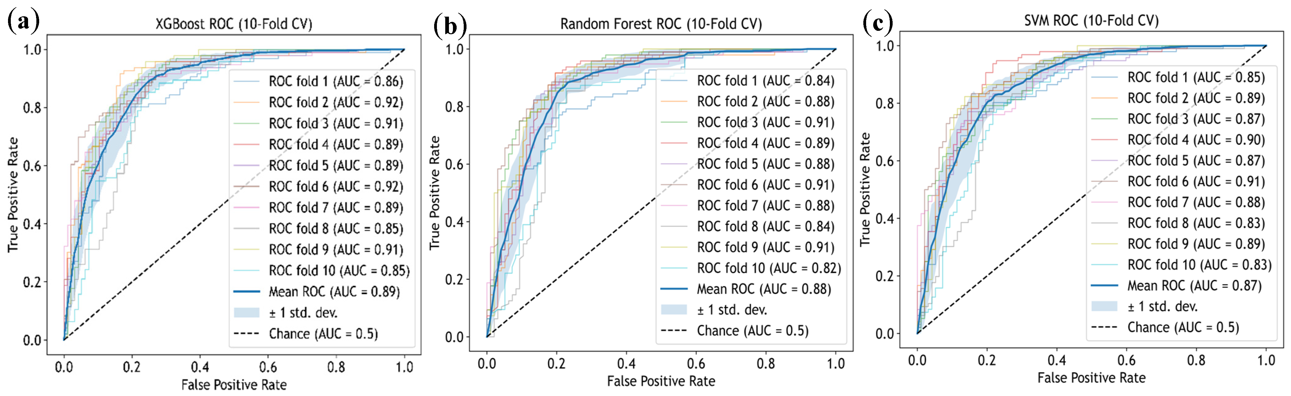
Groundwater potential zone maps are generally validated using ROC curve analysis [70,126]. Figure 9a–c displays the mean ROC and associated standard deviation, together with ROC curves obtained from the k-fold cross-validation (k = 10) analysis. The 10-fold CV’s ROC curves (Figure 10a–c) show that each model’s predictive performance is consistent. With AUC values that vary from 0.85 to 0.92 and an average AUC of 0.89, the XGBoost model exhibits the highest stability and accuracy. The clustering of the ROC around the upper-left corner indicates high true positive rates at low false positive rates. The narrow dispersion rate reflects model stability and low sensitivity to variation in sampling [62].

RF also exhibits a high performance with AUC values ranging from 0.82 to 0.91 (mean AUC = 0.88). Compared to the XGBoost, the RF curves are generally well-clustered with slightly greater dispersion, which suggests moderate sensitivity to sampling variations. However, the model maintains high discriminatory and predictive performance. Comparatively lower performance (mean AUC = 0.87) and wider spread is exhibited by the SVM. The ROC curves show relatively excellent dispersion, which demonstrates high sensitivity to variation in the training subsets. The model (SVM) indicates low capacity to capture complex non-linear relationships. Across all the models, the average ROC curves are above the random baseline (AUC = 0.5) which support their predictive ability.

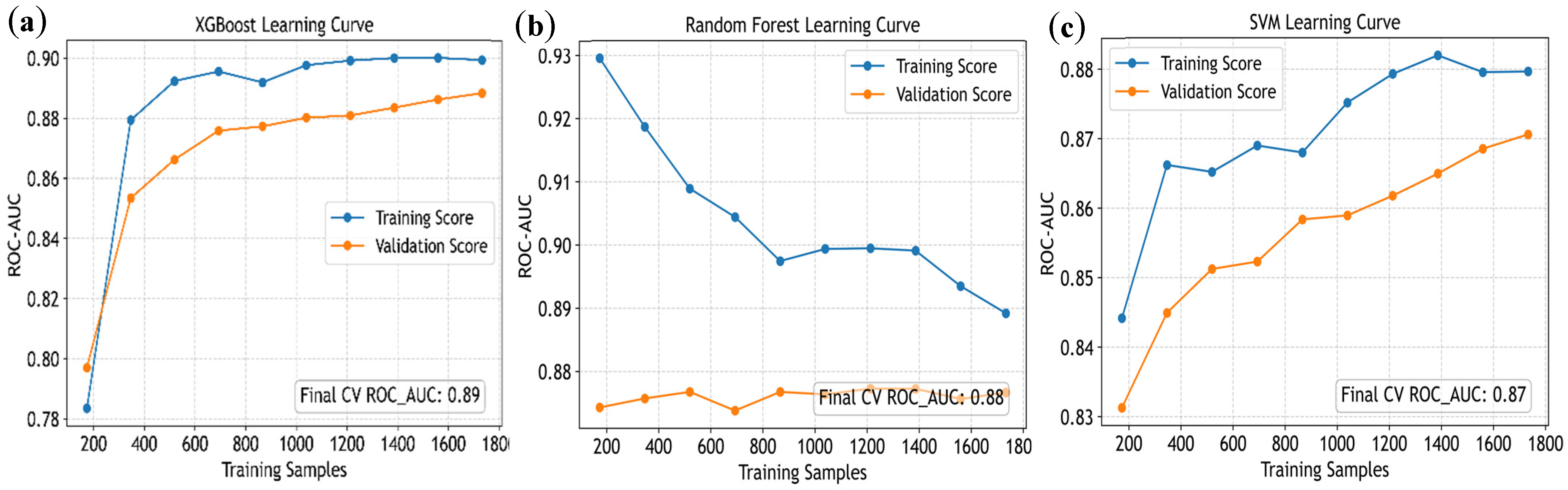
The learning curves (Figure 11a–c) display the variation in training and validation ROC-AUC scores as sample size increases. For the RF model, the training score decreases gradually towards 0.89, while the validation score stabilises around 0.88. The RF model displays a decreasing gap between training and validation scores, which indicates minimal overfitting and stable convergence. A stable learning behaviour was displayed by the XGBoost model, with training and validation curves gradually converging and the AUC reaching 0.89. The narrow gap indicates minimal overfitting and high generalisation ability. The convergence pattern indicates that the model leverages increasing training data to capture complex feature interactions. Both training and validation scores increased gradually with sample size in the SVM model, with AUC approaching 0.87. The small gap between the curves signifies reasonable generalisation and the lower performance reflects limited flexibility in modelling relationships within the dataset. The combined cross-validation and learning curves analysis indicates that all the models exhibit a stable training behaviour and achieve performance convergence. The findings from the analysis demonstrate that the adopted validation framework mitigated bias associated with a single train–test split and provides a basis for model selection and spatial prediction.

4. Discussion

The lithology and aquifer’s permeability of the subsurface strata generally control the occurrence and movement of groundwater [127]. Numerous factors, including geology, topography, fractures, drainage pattern, land cover and climate, control groundwater movement in fractured bedrock aquifers [128]. Since approximately 85% of the FCT is made up of basement complex terrain, which exhibits very low primary porosity, the integration of geophysically derived parameters (depth to bedrock and aquifer thickness) to the groundwater influencing factors improved the model reliability and representation of subsurface conditions.

The GWPZ map generated by the three machine learning models (XGBoost, RF and SVM) exhibits a spatial pattern that reflects the hydrogeological settings of the study area. The southwestern and western sectors delineated as very high to high GWPZ are characterised by gentle slopes, thicker aquifer layer and favourable drainage conditions that improve infiltration and storage. In contrast, the southeastern and northeastern margins characterised by steeper slopes and limited weathering are classified as low to very low groundwater potential areas due to high runoff and lower recharge capacity. The central portion of the study area is dominated by the moderate class.

The spatial pattern exhibited by the models is supported by the multicollinearity assessment (Section 3.2), which proves the weak correlation between predictor variables, which means each factor contributes complementary information in the modelling process. This was further reinforced by the feature importance analysis (Section 3.3), where slope, LULC characteristics (vegetation and impervious surfaces) and hydrological factors such as drainage density and proximity to rivers exert dominant control across all models. The relatively lower influence of the lithological variables suggests that groundwater occurrence in the study area is controlled not by lithology alone but by weathering and the interaction between surface and subsurface factors.

These findings are further substantiated by the model validation results. The relatively close harmony in the ROC-AUC values of the models (XGBoost = 0.89; RF = 0.88 and SVM = 0.87) and the observed stability in cross-validation suggest that the predicted GWPZs are free from model overfitting. Good generalisation and convergence, especially for the ensemble models, were confirmed by the learning curve analysis, which showcases their capability in capturing nonlinear relationships that are natural in hydrogeological systems.

The strength of the model became visible when we combined the results of the correlation analysis with the evaluation of the feature importance. Each factor provides unique and independent information in the modelling process, as revealed by the low pairwise correlations (|r| < 0.5), which suggests minimal multicollinearity. Indicators such as slope, vegetation and drainage density display weak correlations with one another, which confirms their role as distinct hydrogeological influences.

Hydrogeologically, the dominance of the slope reflects the role of terrain in regulating infiltration and runoff. Land use/land cover variables (impervious surface, vegetation and bare land), on the other hand, influence groundwater recharge by controlling surface permeability. Drainage density and proximity to river highlight the interconnection of surface and subsurface water dynamics in the region. Although aquifer thickness and depth to bedrock display moderate statistical significance in the model, they remain very important because they govern groundwater storage and movement in basement terrain. Additionally, the influence of lithology on subsurface aquifer development was highlighted by the strong correlation between aquifer thickness and sandstone (r = 0.73).

Generally, the findings highlight the importance of integrating both surface and subsurface hydrogeological factors into groundwater potential modelling and demonstrate that the ensemble-based machine learning approaches can provide reliable spatial predictions in heterogeneous environments.

5. Conclusions

Most sub-Saharan African nations suffer from water shortages, which are often linked to inadequate management rather than scarcity or drought stress. Inadequate management plans and policies, as well as poor knowledge of water resources, have worsened the water crises in most countries in the region. Adequate information on these vital resources is therefore the first step towards sustainable water resource management. This research developed a GIS-based machine learning model for GWPZ mapping in the FCT (Abuja) by integrating geophysical, remote sensing, climatic and hydrogeological data. The findings demonstrate that the three models (XGBoost, RF and SVM) produce groundwater potential maps with spatial patterns that reflect the hydrogeological condition of the study area.

The spatial distribution of the GWPZ showed that the southwestern and western areas of the FCT, exhibit higher groundwater potential. These areas are characterised by gentle slopes, thicker weathered profiles and improved recharge conditions. The southeastern part, characterised by steep slopes, rugged topography, low weathering profile and low recharge rate, displayed very low to low potential. The reliability of the prediction was enhanced, especially in the basement complex part of the study area, where aquifer productivity is influenced by the thickness of the overlying weathered material, by including geophysically derived parameters such as aquifer thickness and depth to bedrock.

Although all the models performed reasonably, the ensemble-based algorithms (XGBoost and Random Forest) outperform the margin-based algorithm (SVM), as indicated in the ROC-AUC and other related metrics. The agreement between spatial predictions, feature-importance results and validation metrics confirms the reliability of the modelling structure. The findings highlight the importance of integrating surface and subsurface variables in groundwater potential assessment, especially in heterogeneous environments.

This study will provide a practical tool that supports decision makers in drafting action plans for sustainable groundwater development and management. The generated GWPZ maps will serve as a guide for groundwater exploration and development, as well as mitigating the risk associated with abortive borehole drilling and water scarcity in the FCT. Areas classified as very high and high GWPZ should be prioritised for groundwater development projects to meet the agricultural, domestic, and industrial needs of the inhabitants. In regions classified as very low and low GWP, water conservation measures should be implemented to prevent overexploitation of the fragile aquifer and track changes in groundwater levels. The inhabitants should also be trained on water management skills such as rainwater harvesting and conservation.

The model framework used in this research could be applied in other parts of the country with similar terrain characteristics; however, in places with different hydrogeological settings and scarce data, some readjustment, cross-regional validation and uncertainty analysis may be required to improve model performance and transferability, because the performance of the models in this study may have been influenced by the quality and quantity of the input data.

References

- Mohammadi-Behzad, H.R.; Charchi, A.; Kalantari, N.; Nejad, A.M.; Vardanjani, H.K. Delineation of Groundwater Potential Zones Using Remote Sensing (RS), Geographical Information System (GIS) and Analytic Hierarchy Process (AHP) Techniques: A Case Study in the Leylia–Keynow Watershed, Southwest of Iran. Carbonates Evaporites 2019, 34, 1307–1319. [Google Scholar] [CrossRef]
- FAO. Review of World Water Resources by Country; FAO: Rome, Italy, 2003. [Google Scholar]
- Sachdeva, S.; Kumar, B. Groundwater Potential Mapping Using Machine Learning Models for Northeastern Karbi Anglong District, Assam, India. In Proceedings of the 2020 2nd International Conference on Advances in Computing, Communication Control and Networking (ICACCCN), Greater Noida, India, 18 December 2020; IEEE: New York, NY, USA, 2020; pp. 116–121. [Google Scholar]
- Achu, A.L.; Reghunath, R.; Thomas, J. Mapping of Groundwater Recharge Potential Zones and Identification of Suitable Site-Specific Recharge Mechanisms in a Tropical River Basin. Earth Syst. Environ. 2020, 4, 131–145. [Google Scholar] [CrossRef]
- Cuthbert, M.O.; Gleeson, T.; Moosdorf, N.; Befus, K.M.; Schneider, A.; Hartmann, J.; Lehner, B. Global Patterns and Dynamics of Climate–Groundwater Interactions. Nat. Clim. Change 2019, 9, 137–141. [Google Scholar] [CrossRef]
- Sankar, K.; Karunanidhi, D.; Kalaivanan, K.; Subramani, T.; Shanthi, D.; Balamurugan, P. Integrated Hydrogeophysical and GIS Based Demarcation of Groundwater Potential and Vulnerability Zones in a Hard Rock and Sedimentary Terrain of Southern India. Chemosphere 2023, 316, 137305. [Google Scholar] [CrossRef]
- Ajay Kumar, V.; Mondal, N.C.; Ahmed, S. Identification of Groundwater Potential Zones Using RS, GIS and AHP Techniques: A Case Study in a Part of Deccan Volcanic Province (DVP), Maharashtra, India. J. Indian Soc. Remote Sens. 2020, 48, 497–511. [Google Scholar] [CrossRef]
- Naghibi, S.A.; Pourghasemi, H.R.; Abbaspour, K. A Comparison between Ten Advanced and Soft Computing Models for Groundwater Qanat Potential Assessment in Iran Using R and GIS. Theor. Appl. Clim. 2018, 131, 967–984. [Google Scholar] [CrossRef]
- Akter, A.; Uddin, A.M.H.; Wahid, K.B.; Ahmed, S. Predicting Groundwater Recharge Potential Zones Using Geospatial Technique. Sustain. Water Resour. Manag. 2020, 6, 24. [Google Scholar] [CrossRef]
- Chaudhary, B.S.; Kumar, S. Identification of Groundwater Potential Zones Using Remote Sensing and GIS of K-J Watershed, India. J. Geol. Soc. India 2018, 91, 717–721. [Google Scholar] [CrossRef]
- Kumar, M.; Singh, P.; Singh, P. Integrating GIS and Remote Sensing for Delineation of Groundwater Potential Zones in Bundelkhand Region, India. Egypt. J. Remote Sens. Space Sci. 2022, 25, 387–404. [Google Scholar] [CrossRef]
- Rane, N.L.; Jayaraj, G.K. Comparison of Multi-Influence Factor, Weight of Evidence and Frequency Ratio Techniques to Evaluate Groundwater Potential Zones of Basaltic Aquifer Systems. Environ. Dev. Sustain. 2022, 24, 2315–2344. [Google Scholar] [CrossRef]
- Fang, Z.; Wang, Y.; Peng, L.; Hong, H. Integration of Convolutional Neural Network and Conventional Machine Learning Classifiers for Landslide Susceptibility Mapping. Comput. Geosci. 2020, 139, 104470. [Google Scholar] [CrossRef]
- Wang, Y.; Fang, Z.; Wang, M.; Peng, L.; Hong, H. Comparative Study of Landslide Susceptibility Mapping with Different Recurrent Neural Networks. Comput. Geosci. 2020, 138, 104445. [Google Scholar] [CrossRef]
- Lohar, S.N.; Panhalkar, S.S.; Patil, A.S. Forest Fire Susceptibility Mapping Using Analytical Hierarchy Process Approach for Chandoli National Park of Maharashtra, India. Res. Sq. 2020. [Google Scholar] [CrossRef]
- Das, S. Comparison among Influencing Factor, Frequency Ratio, and Analytical Hierarchy Process Techniques for Groundwater Potential Zonation in Vaitarna Basin, Maharashtra, India. Groundw. Sustain. Dev. 2019, 8, 617–629. [Google Scholar] [CrossRef]
- Ghosh, B. Spatial Mapping of Groundwater Potential Using Data-Driven Evidential Belief Function, Knowledge-Based Analytic Hierarchy Process and an Ensemble Approach. Environ. Earth Sci. 2021, 80, 625. [Google Scholar] [CrossRef]
- Rahmati, O.; Pourghasemi, H.R.; Melesse, A.M. Application of GIS-Based Data Driven Random Forest and Maximum Entropy Models for Groundwater Potential Mapping: A Case Study at Mehran Region, Iran. CATENA 2016, 137, 360–372. [Google Scholar] [CrossRef]
- Azimi, S.; Azhdary Moghaddam, M.; Hashemi Monfared, S.A. Spatial Assessment of the Potential of Groundwater Quality Using Fuzzy AHP in GIS. Arab. J. Geosci. 2018, 11, 142. [Google Scholar] [CrossRef]
- Şener, E.; Şener, Ş.; Davraz, A. Groundwater Potential Mapping by Combining Fuzzy-Analytic Hierarchy Process and GIS in Beyşehir Lake Basin, Turkey. Arab. J. Geosci. 2018, 11, 187. [Google Scholar] [CrossRef]
- Lee, S.; Hong, S.-M.; Jung, H.-S. GIS-Based Groundwater Potential Mapping Using Artificial Neural Network and Support Vector Machine Models: The Case of Boryeong City in Korea. Geocarto Int. 2018, 33, 847–861. [Google Scholar] [CrossRef]
- Naghibi, S.A.; Pourghasemi, H.R.; Dixon, B. GIS-Based Groundwater Potential Mapping Using Boosted Regression Tree, Classification and Regression Tree, and Random Forest Machine Learning Models in Iran. Environ. Monit. Assess. 2016, 188, 44. [Google Scholar] [CrossRef]
- Panahi, M.; Sadhasivam, N.; Pourghasemi, H.R.; Rezaie, F.; Lee, S. Spatial Prediction of Groundwater Potential Mapping Based on Convolutional Neural Network (CNN) and Support Vector Regression (SVR). J. Hydrol. 2020, 588, 125033. [Google Scholar] [CrossRef]
- Prasad, P.; Loveson, V.J.; Kotha, M.; Yadav, R. Application of Machine Learning Techniques in Groundwater Potential Mapping along the West Coast of India. GIScience Remote Sens. 2020, 57, 735–752. [Google Scholar] [CrossRef]
- NGDPR. Nigerian Gross Open Data for Africa; National Bureau of Statistics: Abuja, Nigeria, 2020.
- Alagbe, S.A. The Geology of Jidu-Gidan Anfani-Karumo District of the FCT with Emphasis on the Relationship of Porphyroblastic and Non-Porphyroblastic Rocks; Ahmadu Bello University: Zaria, Nigeria, 1979. [Google Scholar]
- Dada, S.S. Proterozoic Evolution of the Nigeria—Boborema Province. Geol. Soc. Lond. Spec. Publ. 2008, 294, 121–136. [Google Scholar] [CrossRef]
- Rahaman, M.A.O.; Fadiya, S.L.; Adekola, S.A.; Coker, S.J.; Bale, R.B.; Olawoki, O.A.; Omada, I.J.; Obaje, N.G.; Akinsanpe, O.T.; Ojo, G.A.; et al. A Revised Stratigraphy of the Bida Basin, Nigeria. J. Afr. Earth Sci. 2019, 151, 67–81. [Google Scholar] [CrossRef]
- Chilton, P.J.; Foster, S.S.D. Hydrogeological Characterisation and Water-Supply Potential of Basement Aquifers in Tropical Africa. Hydrogeol. J. 1995, 3, 36–49. [Google Scholar] [CrossRef]
- Eduvie, M.O.; Olabode, T.; Yaya, O.O. Assessment of Groundwater Potentials of Abuja and Environs. In Towards the Millennium Development Goals: Actions for Water and Environmental Sanitation; Loughborough University: Abuja, Nigeria, 2003; pp. 130–132. [Google Scholar]
- Dan-Hassan, M.A. Aspect of the Hydrogeology of the Federal Capital Territory Abuja, Nigeria; Ahmadu Bello University Press: Zaria, Nigeria, 2015. [Google Scholar]
- Obaje, N.G. Geology and Mineral Resources of Nigeria; Springer: Berlin/Heidelberg, Germany, 2009. [Google Scholar]
- Aweda, A.K.; Jatau, B.S.; Goki, N.G.; Bashir, I.Y. Application of VES and 2D Resistivity Methods for Groundwater Exploration in Kutigi-Enagi Region, Northern Bida Basin, Nigeria. Saudi J. Eng. Technol. 2023, 8, 29–40. [Google Scholar] [CrossRef]
- Agbelade, A.D.; Onyekwelu, J.C.; Oyun, M.B. Tree Species Richness, Diversity, and Vegetation Index for Federal Capital Territory, Abuja, Nigeria. Int. J. For. Res. 2017, 2017, 4549756. [Google Scholar] [CrossRef]
- Agunleti, Y.S.; Arikawe, E.A. Groundwater Targeting Within the Basement Complex Rocks of Federal Capital Territory Abuja Using Remotely Sensed and Vertical Electrical Sounding Data. Int. J. Technol. Enhanc. Emerg. Eng. Res. 2014, 2, 38–47. [Google Scholar]
- FCT. Handbook Federal Capital Territory, Abuja: Background, History, and Progress; Garkida Press Ltd.: Abuja, Nigeria, 1994. [Google Scholar]
- Jimoh, O.D.; Wojuola, O.A. Shallow Aquifer Resources in the Federal Capital Territory of Nigeria. Water Environ. J. 2009, 23, 41–45. [Google Scholar] [CrossRef]
- CIWAT. Water Supply Master Plan of Abuja, Nigeria; CIWAT Nigeria Ltd.: Abuja, Nigeria, 2010. [Google Scholar]
- Yaya, O.O. Impact of Urbanization on the Quality of Groundwater Resources of the Federal Capital Territory, Abuja, Nigeria. Unpublished Research Proposal Report. 2006.
- Omeje, M.; Husin, W.; Noorddin, I.; Oha, I.A.; Onwuka, O.S.; Ugwuoke, P.E.; Meludu, O. Geoelectrical Investigation of Aquifer Problems in Gosa Area of Abuja, North Central, Nigeria. Int. J. Phys. Sci. 2013, 8, 549–559. [Google Scholar] [CrossRef]
- Raji, W.O.; Abdulkadir, K.A. Evaluation of Groundwater Potential of Bedrock Aquifers in Geological Sheet 223 Ilorin, Nigeria, Using Geo-Electric Sounding. Appl. Water Sci. 2020, 10, 220. [Google Scholar] [CrossRef]
- Sunkari, E.D.; Kore, B.M.; Abioui, M. Hydrogeophysical Appraisal of Groundwater Potential in the Fractured Basement Aquifer of the Federal Capital Territory, Abuja, Nigeria. Results Geophys. Sci. 2021, 5, 100012. [Google Scholar] [CrossRef]
- Jyrkama, M.I.; Sykes, J.F.; Normani, S.D. Recharge Estimation for Transient Ground Water Modeling. Groundwater 2002, 40, 638–648. [Google Scholar] [CrossRef] [PubMed]
- Olorunfemi, M.O.; Fasuyi, S.A. Aquifer Types and the Geo-Electric/Hydrogeologic Characteristics of Part of the Central Basement Terrain of Nigeria (Niger State). J. Afr. Earth Sci. 1993, 16, 309–317. [Google Scholar] [CrossRef]
- Zohdy, A.A.R.; Eaton, G.P.; Mabey, D.R. Application of Surface Geophysics to Ground-Water Investigations; U.S. Government Printing Office: Washington, DC, USA, 1974.
- Ibrahim, D.; Nemoto, T.; Raghavan, V. Hydrogeophysical Analysis of Vertical Electrical Soundings for Groundwater Potential and Aquifer Vulnerability Evaluation in the Federal Capital Territory, Abuja, Nigeria. Int. J. Geoinform. 2025, 21, 83–96. [Google Scholar] [CrossRef]
- Bobachev, C. IPI2Win: A Windows Software for an Automatic Interpretation of Resistivity Sounding Data. Ph.D. Thesis, Moscow State University, Moscow, Russia, 2002. [Google Scholar]
- Fashae, O.A.; Tijani, M.N.; Talabi, A.O.; Adedeji, O.I. Delineation of Groundwater Potential Zones in the Crystalline Basement Terrain of SW-Nigeria: An Integrated GIS and Remote Sensing Approach. Appl. Water Sci. 2014, 4, 19–38. [Google Scholar] [CrossRef]
- Magesh, N.S.; Chandrasekar, N.; Soundranayagam, J.P. Delineation of Groundwater Potential Zones in Theni District, Tamil Nadu, Using Remote Sensing, GIS and MIF Techniques. Geosci. Front. 2012, 3, 189–196. [Google Scholar] [CrossRef]
- Roy, A.; Keesari, T.; Sinha, U.K.; Sabarathinam, C. Delineating Groundwater Prospect Zones in a Region with Extreme Climatic Conditions Using GIS and Remote Sensing Techniques: A Case Study from Central India. J. Earth Syst. Sci. 2019, 128, 201. [Google Scholar] [CrossRef]
- Díaz-Alcaide, S.; Martínez-Santos, P. Review: Advances in Groundwater Potential Mapping. Hydrogeol. J. 2019, 27, 2307–2324. [Google Scholar] [CrossRef]
- Belmessaoud, B. A Novel Approach for the Determination of Groundwater Potential. Master’s Thesis, University Kasdi Merbah Ouargla, Ouargla, Algeria, 2022. [Google Scholar]
- Funk, C.; Peterson, P.; Landsfeld, M.; Pedreros, D.; Verdin, J.; Shukla, S.; Husak, G.; Rowland, J.; Harrison, L.; Hoell, A.; et al. The Climate Hazards Infrared Precipitation with Stations a New Environmental Record for Monitoring Extremes. Sci. Data 2015, 2, 150066. [Google Scholar] [CrossRef] [PubMed]
- Adeyeye, O.A.; Ikpokonte, E.A.; Arabi, S.A. GIS-Based Groundwater Potential Mapping within Dengi Area, North Central Nigeria. Egypt. J. Remote Sens. Space Sci. 2019, 22, 175–181. [Google Scholar] [CrossRef]
- Shrestha, N. Detecting Multicollinearity in Regression Analysis. AJAMS 2020, 8, 39–42. [Google Scholar] [CrossRef]
- Kalnins, A. Multicollinearity: How Common Factors Cause Type 1 Errors in Multivariate Regression. Strateg. Manag. J. 2018, 39, 2362–2385. [Google Scholar] [CrossRef]
- Devore, J.L. Probability and Statistics for Engineering and the Sciences, 8th ed.; Cengage Learning: Boston, MA, USA, 2011. [Google Scholar]
- Field, A. Discovering Statistics Using IBM SPSS Statistics: And Sex and Drugs and Rock “n” Roll, 4th ed.; Mobile Study; Sage: Los Angeles, CA, USA; London, UK; New Delhi, India; Singapore; Washington, DC, USA, 2013; ISBN 978-1-4462-4918-5. [Google Scholar]
- Foster, S.; Tuinhof, A.; Garduño, H. Sustainable Groundwater Management: Lessons from Practice. In Groundwater Development in Sub-Saharan Africa: A Strategic Overview of Key Issues and Major Needs; GW-MATE Case Profile Collection; World Bank (GW-MATE): Washington, DC, USA, 2006. [Google Scholar]
- Mallick, J.; Talukdar, S.; Alsubih, M.; Almesfer, M.K.; Shahfahad; Hang, H.T.; Rahman, A. Integration of Statistical Models and Ensemble Machine Learning Algorithms (MLAs) for Developing the Novel Hybrid Groundwater Potentiality Models: A Case Study of Semi-Arid Watershed in Saudi Arabia. Geocarto Int. 2022, 37, 6442–6473. [Google Scholar] [CrossRef]
- Pandala, S.R. LazyPredict: Build and Compare Machine Learning Models in One Line of Code; GitHub Repository. 2020. Available online: https://github.com/shankarpandala/lazypredict (accessed on 20 September 2025).
- Chen, T.; Guestrin, C. XGBoost: A Scalable Tree Boosting System. In Proceedings of the Proceedings of the 22nd ACM SIGKDD International Conference on Knowledge Discovery and Data Mining; ACM: San Francisco, CA, USA, 2016; pp. 785–794. [Google Scholar]
- Song, Y.; Li, H.; Xu, P.; Liu, D. A Method of Intrusion Detection Based on WOA-XGBoost Algorithm. Discret. Dyn. Nat. Soc. 2022, 2022, 5245622. [Google Scholar] [CrossRef]
- Rasool, U.; Yin, X.; Xu, Z.; Rasool, M.A.; Senapathi, V.; Hussain, M.; Siddique, J.; Trabucco, J.C. Mapping of Groundwater Productivity Potential with Machine Learning Algorithms: A Case Study in the Provincial Capital of Baluchistan, Pakistan. Chemosphere 2022, 303, 135265. [Google Scholar] [CrossRef] [PubMed]
- Li, N.; Li, B.; Gao, L. Transient Stability Assessment of Power System Based on XGBoost and Factorization Machine. IEEE Access 2020, 8, 28403–28414. [Google Scholar] [CrossRef]
- Lin, L.; Liang, Y.; Liu, L.; Zhang, Y.; Xie, D.; Yin, F.; Ashraf, T. Estimating PM2.5 Concentrations Using the Machine Learning RF-XGBoost Model in Guanzhong Urban Agglomeration, China. Remote Sens. 2022, 14, 5239. [Google Scholar] [CrossRef]
- Wu, S.; Yuan, Q.; Yan, Z.; Xu, Q. Analyzing Accident Injury Severity via an Extreme Gradient Boosting (XGBoost) Model. J. Adv. Transp. 2021, 2021, 3771640. [Google Scholar] [CrossRef]
- Jiang, H.; He, Z.; Ye, G.; Zhang, H. Network Intrusion Detection Based on PSO-Xgboost Model. IEEE Access 2020, 8, 58392–58401. [Google Scholar] [CrossRef]
- Breiman, L. Random Forests. Mach. Learn. 2001, 45, 5–32. [Google Scholar] [CrossRef]
- Naghibi, S.A.; Moghaddam, D.D.; Kalantar, B.; Pradhan, B.; Kisi, O. A Comparative Assessment of GIS-Based Data Mining Models and a Novel Ensemble Model in Groundwater Well Potential Mapping. J. Hydrol. 2017, 548, 471–483. [Google Scholar] [CrossRef]
- Golkarian, A.; Naghibi, S.A.; Kalantar, B.; Pradhan, B. Groundwater Potential Mapping Using C5.0, Random Forest, and Multivariate Adaptive Regression Spline Models in GIS. Environ. Monit. Assess. 2018, 190, 149. [Google Scholar] [CrossRef]
- Sameen, M.I.; Pradhan, B.; Lee, S. Self-Learning Random Forests Model for Mapping Groundwater Yield in Data-Scarce Areas. Nat. Resour. Res. 2019, 28, 757–775. [Google Scholar] [CrossRef]
- Sameen, M.I.; Pradhan, B.; Lee, S. Application of Convolutional Neural Networks Featuring Bayesian Optimization for Landslide Susceptibility Assessment. CATENA 2020, 186, 104249. [Google Scholar] [CrossRef]
- Catani, F.; Lagomarsino, D.; Segoni, S.; Tofani, V. Landslide Susceptibility Estimation by Random Forests Technique: Sensitivity and Scaling Issues. Nat. Hazards Earth Syst. Sci. 2013, 13, 2815–2831. [Google Scholar] [CrossRef]
- Naghibi, S.A.; Pourghasemi, H.R. A Comparative Assessment Between Three Machine Learning Models and Their Performance Comparison by Bivariate and Multivariate Statistical Methods in Groundwater Potential Mapping. Water Resour. Manag. 2015, 29, 5217–5236. [Google Scholar] [CrossRef]
- Mojaddadi, H.; Pradhan, B.; Nampak, H.; Ahmad, N.; Ghazali, A.H.B. Ensemble Machine-Learning-Based Geospatial Approach for Flood Risk Assessment Using Multi-Sensor Remote-Sensing Data and GIS. Geomat. Nat. Hazards Risk 2017, 8, 1080–1102. [Google Scholar] [CrossRef]
- Tehrany, M.S.; Pradhan, B.; Jebur, M.N. Flood Susceptibility Mapping Using a Novel Ensemble Weights-of-Evidence and Support Vector Machine Models in GIS. J. Hydrol. 2014, 512, 332–343. [Google Scholar] [CrossRef]
- Su, H.; Li, X.; Yang, B.; Wen, Z. Wavelet Support Vector Machine-Based Prediction Model of Dam Deformation. Mech. Syst. Signal Process. 2018, 110, 412–427. [Google Scholar] [CrossRef]
- Marjanović, M.; Kovačević, M.; Bajat, B.; Voženílek, V. Landslide Susceptibility Assessment Using SVM Machine Learning Algorithm. Eng. Geol. 2011, 123, 225–234. [Google Scholar] [CrossRef]
- Tehrany, M.S.; Pradhan, B.; Mansor, S.; Ahmad, N. Flood Susceptibility Assessment Using GIS-Based Support Vector Machine Model with Different Kernel Types. CATENA 2015, 125, 91–101. [Google Scholar] [CrossRef]
- Hong, H.; Pradhan, B.; Bui, D.T.; Xu, C.; Youssef, A.M.; Chen, W. Comparison of Four Kernel Functions Used in Support Vector Machines for Landslide Susceptibility Mapping: A Case Study at Suichuan Area (China). Geomat. Nat. Hazards Risk 2017, 8, 544–569. [Google Scholar] [CrossRef]
- Samui, P. Slope Stability Analysis: A Support Vector Machine Approach. Environ. Geol. 2008, 56, 255–267. [Google Scholar] [CrossRef]
- Yao, X.; Tham, L.G.; Dai, F.C. Landslide Susceptibility Mapping Based on Support Vector Machine: A Case Study on Natural Slopes of Hong Kong, China. Geomorphology 2008, 101, 572–582. [Google Scholar] [CrossRef]
- Chen, W.; Li, H.; Hou, E.; Wang, S.; Wang, G.; Panahi, M.; Li, T.; Peng, T.; Guo, C.; Niu, C.; et al. GIS-Based Groundwater Potential Analysis Using Novel Ensemble Weights-of-Evidence with Logistic Regression and Functional Tree Models. Sci. Total Environ. 2018, 634, 853–867. [Google Scholar] [CrossRef]
- Cortes, C.; Vapnik, V. Support-Vector Networks. Mach. Learn. 1995, 20, 273–297. [Google Scholar] [CrossRef]
- Hsu, C.-W.; Chang, C.-C.; Lin, C.-J. A Practical Guide to Support Vector Classification; Department of Computer Science; National Taiwan University: Taipei, Taiwan, 2003. [Google Scholar]
- Vapnik, V.N. Statistical Learning Theory; John Wiley & Sons: New York, NY, USA, 1998. [Google Scholar]
- Chen, W.; Panahi, M.; Khosravi, K.; Pourghasemi, H.R.; Rezaie, F.; Parvinnezhad, D. Spatial Prediction of Groundwater Potentiality Using ANFIS Ensembled with Teaching-Learning-Based and Biogeography-Based Optimization. J. Hydrol. 2019, 572, 435–448. [Google Scholar] [CrossRef]
- Egan, J.P. Signal Detection Theory and ROC Analysis; Academic Press: New York, NY, USA, 1975. [Google Scholar]
- Youssef, A.M.; Pourghasemi, H.R.; Pourtaghi, Z.S.; Al-Katheeri, M.M. Landslide Susceptibility Mapping Using Random Forest, Boosted Regression Tree, Classification and Regression Tree, and General Linear Models and Comparison of Their Performance at Wadi Tayyah Basin, Asir Region, Saudi Arabia. Landslides 2016, 13, 839–856. [Google Scholar] [CrossRef]
- Fawcett, T. An Introduction to ROC Analysis. Pattern Recognit. Lett. 2006, 27, 861–874. [Google Scholar] [CrossRef]
- Kohavi, R. A Study of Cross-Validation and Bootstrap for Accuracy Estimation and Model Selection. In Proceedings of the 14th International Joint Conference on Artificial Intelligence (IJCAI); Morgan Kaufmann Publishers Inc.: San Francisco, CA, USA, 1995; pp. 1137–1143. [Google Scholar]
- Hastie, T.; Tibshirani, R.; Friedman, J. The Elements of Statistical Learning; Springer Series in Statistics; Springer: New York, NY, USA, 2009; ISBN 978-0-387-84857-0. [Google Scholar]
- James, G.; Witten, D.; Hastie, T.; Tibshirani, R. An Introduction to Statistical Learning: With Applications in R; Springer Texts in Statistics; Springer: New York, NY, USA, 2021; ISBN 978-1-0716-1417-4. [Google Scholar]
- Manning, C.D.; Raghavan, P.; Schütze, H. Introduction to Information Retrieval; Cambridge University Press: Cambridge, UK, 2008; ISBN 978-0-521-86571-5. [Google Scholar]
- Goodfellow, I.; Bengio, Y.; Courville, A. Deep Learning; Adaptive Computation and Machine Learning; The MIT Press: Mass, MI, USA, 2016; ISBN 978-0-262-03561-3. [Google Scholar]
- Ajibade, A.C.; Wright, J.B. The Togo-Benin-Nigeria Shield: Evidence of Crustal Aggregation in the Pan-African Belt. Tectonophysics 1989, 165, 125–129. [Google Scholar] [CrossRef]
- Rahaman, M.A. Precambrian Geology of Nigeria; Geological Survey of Nigeria Publications: Abuja, Nigeria, 1988. [Google Scholar]
- Edet, A.E.; Teme, S.C.; Okereke, C.S.; Esu, E.O. Lineament Analysis for Groundwater Exploration in Precambrian Oban Massif and Obudu Plateau, SE Nigeria. Int. J. Rock. Mech. Min. Sci. Geomech. Abstr. 1996, 33, A215. [Google Scholar] [CrossRef]
- Offodile, M.E. Groundwater Study and Development in Nigeria, 2nd ed.; Mecon Geology & Engineering Services Ltd.: Jos, Nigeria, 2002. [Google Scholar]
- Wright, E.P. The Hydrogeology of Crystalline Basement Aquifers in Africa. Geol. Soc. London Spéc. Publ. 1992, 66, 1–27. [Google Scholar] [CrossRef]
- Ideki, O.; Weli, V.E. Analysis of Rainfall Variability Using Remote Sensing and GIS in North Central Nigeria. Atmos. Clim. Sci. 2019, 9, 191–201. [Google Scholar] [CrossRef]
- Nicholson, S.E. The West African Sahel: A Review of Recent Studies on the Rainfall Regime and Its Interannual Variability. ISRN Meteorol. 2013, 2013, 453521. [Google Scholar] [CrossRef]
- Boori, M.S.; Choudhary, K.; Kupriyanov, A. Mapping of Groundwater Potential Zone Based on Remote Sensing and GIS Techniques: A Case Study of Kalmykia, Russia. Opt. Mem. Neural Netw. 2019, 28, 36–49. [Google Scholar] [CrossRef]
- Machiwal, D.; Jha, M.K.; Mal, B.C. Assessment of Groundwater Potential in a Semiarid Region of India Using Remote Sensing, GIS and MCDM Techniques. Water Resour. Manag. 2011, 25, 1359–1386. [Google Scholar] [CrossRef]
- Ghosh, P.K.; Bandyopadhyay, S.; Jana, N.C. Mapping of Groundwater Potential Zones in Hard Rock Terrain Using Geoinformatics: A Case of Kumari Watershed in Western Part of West Bengal. Model. Earth Syst. Environ. 2016, 2, 1. [Google Scholar] [CrossRef]
- Kaliraj, S.; Chandrasekar, N.; Magesh, N.S. Identification of Potential Groundwater Recharge Zones in Vaigai Upper Basin, Tamil Nadu, Using GIS-Based Analytical Hierarchical Process (AHP) Technique. Arab. J. Geosci. 2014, 7, 1385–1401. [Google Scholar] [CrossRef]
- Arnold, C.L.; Gibbons, C.J. Impervious Surface Coverage: The Emergence of a Key Environmental Indicator. J. Am. Plan. Assoc. 1996, 62, 243–258. [Google Scholar] [CrossRef]
- Kaur, L.; Rishi, M.S.; Singh, G.; Nath Thakur, S. Groundwater Potential Assessment of an Alluvial Aquifer in Yamuna Sub-Basin (Panipat Region) Using Remote Sensing and GIS Techniques in Conjunction with Analytical Hierarchy Process (AHP) and Catastrophe Theory (CT). Ecol. Indic. 2020, 110, 105850. [Google Scholar] [CrossRef]
- Thomas, M.F.; Thomas, M.F. Geomorphology in the Tropics: A Study of Weathering and Denudation in Low Latitudes; Wiley: Chichester, UK, 1996; ISBN 978-0-471-93035-8. [Google Scholar]
- Deepa, S.; Venkateswaran, S.; Ayyandurai, R.; Kannan, R.; Vijay Prabhu, M. Groundwater Recharge Potential Zones Mapping in Upper Manimuktha Sub Basin Vellar River Tamil Nadu India Using GIS and Remote Sensing Techniques. Model. Earth Syst. Environ. 2016, 2, 137. [Google Scholar] [CrossRef]
- Rais, S.; Javed, A. Identification of Artificial Recharge Sites in Manchi Basin, Eastern Rajasthan (India) Using Remote Sensing and GIS Techniques. JGIS 2014, 6, 162–175. [Google Scholar] [CrossRef]
- Kirubakaran, M.; Johnny, J.C.; Ashokraj, C.; Arivazhagan, S. A Geostatistical Approach for Delineating the Potential Groundwater Recharge Zones in the Hard Rock Terrain of Tirunelveli Taluk, Tamil Nadu, India. Arab. J. Geosci. 2016, 9, 382. [Google Scholar] [CrossRef]
- Shailaja, G.; Kadam, A.K.; Gupta, G.; Umrikar, B.N.; Pawar, N.J. Integrated Geophysical, Geospatial and Multiple-Criteria Decision Analysis Techniques for Delineation of Groundwater Potential Zones in a Semi-Arid Hard-Rock Aquifer in Maharashtra, India. Hydrogeol. J. 2019, 27, 639–654. [Google Scholar] [CrossRef]
- Bagyaraj, M.; Ramkumar, T.; Venkatramanan, S.; Gurugnanam, B. Application of Remote Sensing and GIS Analysis for Identifying Groundwater Potential Zone in Parts of Kodaikanal Taluk, South India. Front. Earth Sci. 2013, 7, 65–75. [Google Scholar] [CrossRef]
- Agarwal, E.; Agarwal, R.; Garg, R.D.; Garg, P.K. Delineation of Groundwater Potential Zone: An AHP/ANP Approach. J. Earth Syst. Sci. 2013, 122, 887–898. [Google Scholar] [CrossRef]
- Das, N.; Mukhopadhyay, S. Application of Multi-Criteria Decision Making Technique for the Assessment of Groundwater Potential Zones: A Study on Birbhum District, West Bengal, India. Environ. Dev. Sustain. 2020, 22, 931–955. [Google Scholar] [CrossRef]
- Todd, D.K.; Mays, L.W. Groundwater Hydrology, 3rd ed.; Wiley India Exclusive (Cbs): Noida, India, 2005. [Google Scholar]
- Prasad, R.K.; Mondal, N.C.; Banerjee, P.; Nandakumar, M.V.; Singh, V.S. Deciphering Potential Groundwater Zone in Hard Rock through the Application of GIS. Environ. Geol. 2008, 55, 467–475. [Google Scholar] [CrossRef]
- Sophocleous, M. Interactions between Groundwater and Surface Water: The State of the Science. Hydrogeol. J. 2002, 10, 52–67. [Google Scholar] [CrossRef]
- Winter, T.C.; Harvey, J.W.; Franke, O.L.; Alley, W.M. Ground Water and Surface Water: A Single Resource; USGS Circular; US Geological Survey: Reston, VA, USA, 1998; ISBN 0-607-89351-1.
- Dormann, C.F.; Elith, J.; Bacher, S.; Buchmann, C.; Carl, G.; Carré, G.; Marquéz, J.R.G.; Gruber, B.; Lafourcade, B.; Leitão, P.J.; et al. Collinearity: A Review of Methods to Deal with It and a Simulation Study Evaluating Their Performance. Ecography 2013, 36, 27–46. [Google Scholar] [CrossRef]
- Gómez-Escalonilla, V.; Vogt, M.-L.; Destro, E.; Isseini, M.; Origgi, G.; Djoret, D.; Martínez-Santos, P.; Holecz, F. Delineation of Groundwater Potential Zones by Means of Ensemble Tree Supervised Classification Methods in the Eastern Lake Chad Basin. Geocarto Int. 2022, 37, 8924–8951. [Google Scholar] [CrossRef]
- Kuhn, M.; Johnson, K. Applied Predictive Modeling; Springer: New York, NY, USA, 2013; ISBN 978-1-4614-6848-6. [Google Scholar]
- Kutner, M.H.; Nachtsheim, C.; Neter, J.; Li, W. Applied Linear Statistical Models, 5th ed.; McGraw-Hill Irwin: Boston, UK, 2005; ISBN 978-0-07-238688-2. [Google Scholar]
- Andualem, T.G.; Demeke, G.G. Groundwater Potential Assessment Using GIS and Remote Sensing: A Case Study of Guna Tana Landscape, Upper Blue Nile Basin, Ethiopia. J. Hydrol. Reg. Stud. 2019, 24, 100610. [Google Scholar] [CrossRef]
- Ozdemir, A. GIS-Based Groundwater Spring Potential Mapping in the Sultan Mountains (Konya, Turkey) Using Frequency Ratio, Weights of Evidence and Logistic Regression Methods and Their Comparison. J. Hydrol. 2011, 411, 290–308. [Google Scholar] [CrossRef]
- Oh, H.-J.; Kim, Y.-S.; Choi, J.-K.; Park, E.; Lee, S. GIS Mapping of Regional Probabilistic Groundwater Potential in the Area of Pohang City, Korea. J. Hydrol. 2011, 399, 158–172. [Google Scholar] [CrossRef]