Enhancing Multi-Step Reservoir Inflow Forecasting: A Time-Variant Encoder–Decoder Approach

Abstract

Accurate reservoir inflow forecasting is vital for effective water resource management. Reliable forecasts enable operators to optimize storage and release strategies to meet competing sectoral demands—such as water supply, irrigation, and hydropower scheduling—while also mitigating flood and drought risks. To address this need, in this study, we propose a novel time-variant encoder–decoder (ED) model designed specifically to improve multi-step reservoir inflow forecasting, enabling accurate predictions of reservoir inflows up to seven days ahead. Unlike conventional ED-LSTM and recursive ED-LSTM models, which use fixed encoder parameters or recursively propagate predictions, our model incorporates an adaptive encoder structure that dynamically adjusts to evolving conditions at each forecast horizon. Additionally, we introduce the Expected Baseline Integrated Gradients (EB-IGs) method for variable importance analysis, enhancing interpretability of inflow by incorporating multiple baselines to capture a broader range of hydrometeorological conditions. The proposed methods are demonstrated at several diverse reservoirs across the United States. Our results show that they outperform traditional methods, particularly at longer lead times, while also offering insights into the key drivers of inflow forecasting. These advancements contribute to enhanced reservoir management through improved forecasting accuracy and practical decision-making insights under complex hydroclimatic conditions.

1. Introduction

Reservoir inflow forecasting plays a critical role in effective water resource management, enabling operators to optimize storage and release strategies to meet diverse demands and adapt to changing environmental conditions [1,2]. This forecasting capability is vital for balancing the needs of multiple sectors, including energy production (hydropower scheduling), agriculture, industry, and municipal services, as well as mitigating risks of water shortages and flooding [3,4]. By providing insights into future water availability, forecasting facilitates informed decision-making, allowing reservoir managers to maintain adequate supplies for regular operations while preserving the flexibility to adapt to extreme events [5,6]. Consequently, advancements in inflow forecasting techniques not only enhance operational efficiency but also contribute significantly to water security and resilience, addressing evolving challenges in water resource management.

While physics-based models have traditionally been utilized for hydrologic streamflow forecasting, in recent years, machine learning (ML) techniques have emerged as a powerful tool, particularly for reservoir inflow predictions. Among these ML techniques, the long short-term memory (LSTM) model has gained particular recognition [6,7]. LSTM models incorporate hidden and cell states that enable them to capture and retain long-term dependencies, making them particularly well-suited for analyzing time series data [8]. These models effectively capture the highly nonlinear relationships and temporal dependencies inherent in hydrometeorological variables [7,9,10]. For instance, Kratzert et al. [10] demonstrated the effectiveness of LSTM models in streamflow forecasting, achieving promising results when compared to traditional physically based approaches.

Building upon the strengths of LSTM models, more advanced configurations have been developed to address some of the limitations of single LSTM models. One such architecture is the encoder–decoder (ED) framework, which links two LSTMs (an encoder and a decoder) through a fixed-size vector [11]. This vector encapsulates key hydrometeorological information from the input sequence, thereby enhancing the model’s ability to capture temporal dependencies and enhancing multi-step forecasting accuracy [12,13,14,15,16,17]. For example, Fan et al. [16] applied the ED-LSTM model to forecast multi-step inflows at 30 reservoirs in the Upper Colorado River Basin, USA. The results demonstrate that the ED-LSTM model consistently outperforms the vanilla LSTM model across all forecast horizons. Its ability to process and retain critical hydrometeorological information from long input sequences enables the capture of long-range dependencies, enhancing its effectiveness in multi-step predictions.

Despite their widespread use, ED-LSTM models encounter limitations in certain applications. For instance, Kao et al.’s work demonstrated that the standard ED-LSTM model failed to incorporate available future meteorological data, thus constraining its multi-step forecasting accuracy [12]. To address this, Xiang et al. proposed an enhanced ED-LSTM model that encodes both historical and forecasted meteorological forcing data into one state vector, while encoding runoff data into another [13]. These vectors, along with additional time series like evapotranspiration, are combined into a unified state vector, which serves as input for the decoder to generate multi-step forecasts. However, this structure violates the fundamental cause-and-effect dynamics necessary for accurate predictions [14]. In reality, meteorological variables from future time steps, such as temperature and precipitation, should not influence inflow forecasts at earlier horizons. For example, when forecasting inflow for the jth day, meteorological data beyond the jth day should not affect that forecast, as this could introduce potential inaccuracies.

In addition to this issue, standard ED-LSTM models struggle to adapt to dynamic hydroclimatic conditions. The use of a fixed state vector across all forecast horizons imposes a time-invariant structure, where encoder parameters remain unchanged for each prediction step. This limitation restricts the model’s ability to capture evolving temporal dynamics and complex dependencies, which are critical for accurate multi-step inflow forecasting. Consequently, the model’s capacity to respond to variations in hydrometeorological data and account for long-range dependencies is compromised. To address these challenges, we propose a novel time-variant ED model designed to enhance multi-step ahead inflow forecasts. Our method incorporates a dynamic encoder structure, where the model parameters evolve with each prediction step, allowing the encoder to adapt to varying conditions over time. The dynamically encoded information is then fed into the decoder for predictions at each lead time. By enabling the model to adjust to time-varying dynamics, our method significantly improves the capture of crucial long-term dependencies, essential for accurate multi-step forecasting.

Moreover, improving model interpretability is equally important, especially in understanding how input variables influence inflow forecasts, which provides actionable insights for water resource management [8,18,19,20]. One widely used method for interpreting ML models is SHAP (SHapley Additive exPlanations), valued for its ability to quantify feature importance [21,22]. However, SHAP’s computational demands, particularly in real-time applications with large datasets, can pose challenges due to its reliance on permutation-based calculations [16,23].

To address this computational limitation, we employ gradient-based explanation methods to assess the importance of hydrometeorological variables, offering a more computationally efficient alternative without sacrificing interpretability. Previous studies have used integrated gradients (IG) to analyze input variable importance [10,24,25,26]. IG attributes model predictions to input features by integrating gradients from a baseline to the actual input [27]. However, many studies use a single, fixed baseline, often zero, which can lead to misleading interpretations of feature importance when the baseline does not represent realistic conditions.

In hydrological forecasting, for example, setting the baseline to zero may not always be appropriate, as zero values for inputs such as temperature often do not reflect real-world conditions. To address this issue, we enhance the IG method by incorporating multiple baselines randomly selected from the training data, capturing a broader range of hydrometeorological conditions. This approach improves the robustness and accuracy of feature attribution, providing more reliable insights into how various hydrometeorological factors impact inflow forecasts. By improving interpretability, our method enables a more comprehensive understanding of the drivers behind inflow variability, facilitating more informed and effective decision-making in water resource management.

The remainder of this paper is structured as follows: Section 2 presents the details of the time-variant ED model, along with a brief overview of standard ED models. Section 3 outlines the training dataset used in this study, the numerical experimental design, and the evaluation metrics employed. Section 4 presents the forecast results, including a comparison of the time-variant ED model with ED-LSTM and recursive ED-LSTM models, along with interpretation analysis. Finally, Section 5 provides a discussion of our findings, and Section 6 concludes this study.

2. Methods

2.1. Standard Encoder–Decoder (ED) Models

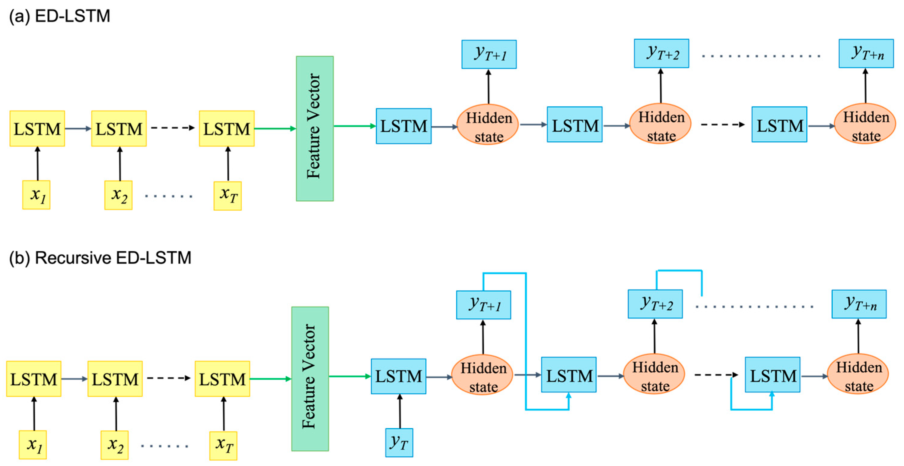
The ED-LSTM model is a widely used architecture for time series forecasting, as illustrated in Figure 1a. In this model, the encoder processes input sequences, such as historical hydrometeorological data, and compresses them into a fixed-length vector that encapsulates essential temporal dependencies. Subsequently, the decoder utilizes this encoded representation to generate multi-step forecasts. An extension of this approach, the Recursive ED-LSTM model, feeds the output of the decoder back into the model as input for subsequent predictions, as illustrated in Figure 1b. Rather than predicting all time steps simultaneously, the recursive ED-LSTM model forecasts one step at a time, incorporating the previous prediction as the input for the next step. A common limitation of standard ED models is their reliance on a fixed historical window, typically the past T days of hydrometeorological data. This static information, while providing a foundational basis for prediction, remains constant across all forecasting steps. Consequently, the model’s ability to capture evolving temporal dynamics may be constrained, as it does not adjust its encoding based on future inputs or varying conditions at different forecast horizons. This limitation can potentially impact the accuracy of multi-step forecasts, particularly in scenarios with large dynamic changes in hydroclimatic variables.

2.2. Time-Variant Encoder–Decoder (ED) Model

To address the limitations of standard ED models in capturing evolving temporal dynamics, we propose a time-variant ED model to enhance multi-step ahead inflow forecasting, as illustrated in Figure 2. This novel approach incorporates dynamic encoder structures that adapt across each forecast horizon, allowing the model to better capture evolving temporal dependencies and adjust to changing hydroclimatic conditions. Compared to standard ED models, where the encoder and decoder operate with fixed parameters across all prediction steps, our time-variant ED model introduces a flexible framework where the encoder parameters are dynamically adjusted for each forecast horizon. Specifically, the decoder generates one-step-ahead predictions based on these time-varying encoded representations, enabling the model to capture temporal dependencies specific to each forecast horizon.

The time-variant ED model preserves the core components of the standard ED architecture, utilizing LSTM models for both the encoder and decoder. For the initial prediction step, the model processes T time steps of historical hydrometeorological variables. As the forecast horizon extends, the model progressively incorporates forecasted hydrometeorological data into the encoder input. For instance, the second-step forecast integrates not only the past hydrometeorological information but also the previously predicted reservoir inflow and meteorological data. This dynamic input strategy ensures a more comprehensive integration of information throughout the forecasting period.

A key feature of our time-variant ED model is its parameter propagation mechanism across forecast horizons. This approach operates on two levels: First, the model weights (including those in the encoder and decoder) from the initial prediction step are used to initialize the subsequent step, providing an informed starting point for further training. Second, the hidden and cell states of the LSTM layers, which capture short-term and long-term dependencies, respectively, are carried forward from one prediction step to the next. This dual propagation strategy ensures continuity in the model’s learning process and maintains stability across multi-step forecasts. By leveraging information from previous steps, the model mitigates parameter drift and preserves its predictive capabilities as it generates forecasts further into the future.

By integrating forecasted hydrometeorological variables into the input sequence for each prediction step, the model becomes better equipped to handle the nonstationary nature of hydrometeorological data and adapt to dynamic hydroclimatic conditions. This approach results in a unique set of parameters for each forecast horizon, allowing the model to capture long-term dependencies specific to each forecast horizon and thus deliver more accurate multi-step inflow forecasts. In summary, the dynamic nature of the time-variant ED model enhances its adaptability and improves both the accuracy and reliability of inflow forecasting, especially in scenarios with rapidly changing hydroclimatic conditions.

2.3. Expected Baseline Integrated Gradients (EB-IG)

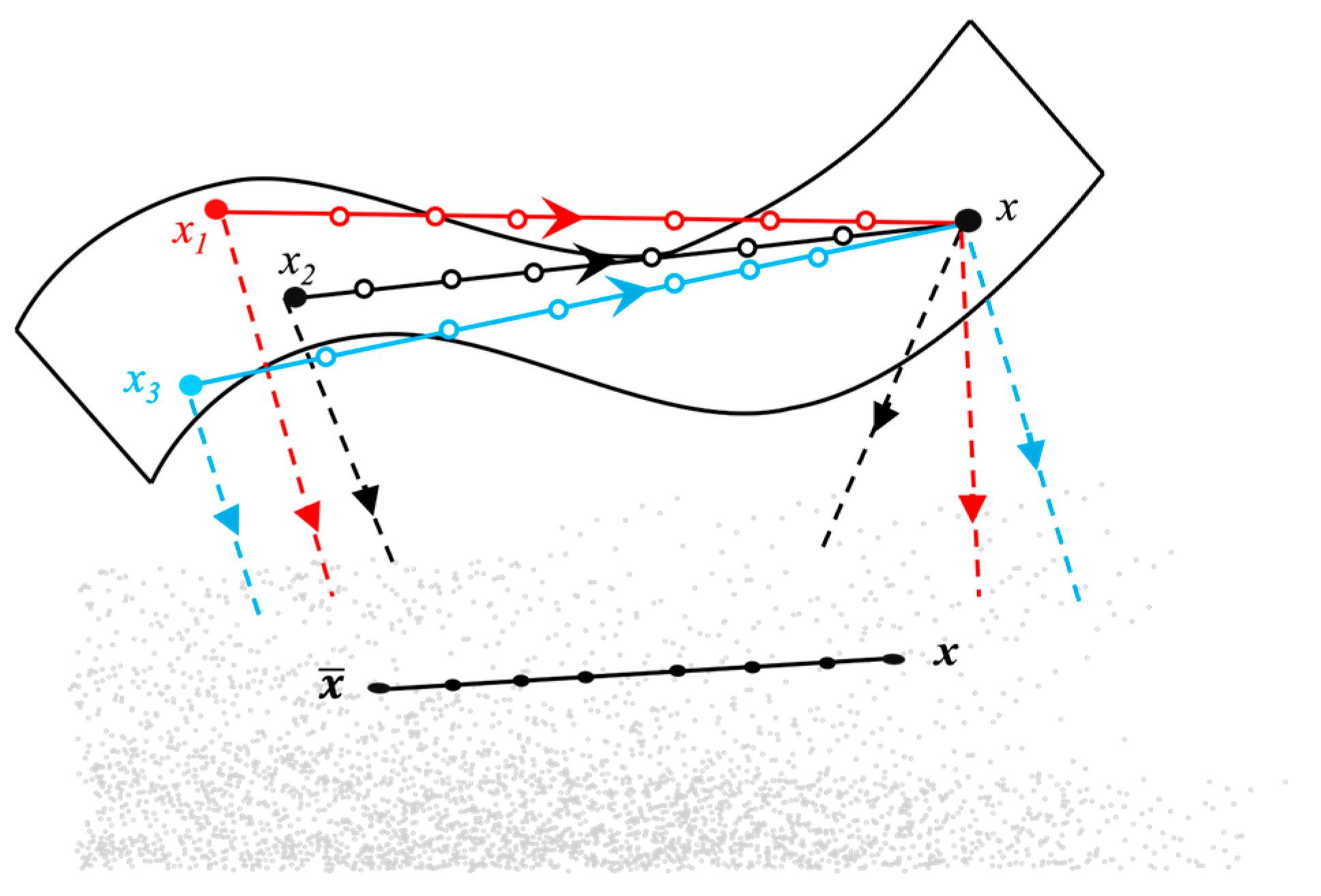
To better understand how hydrometeorological forcings influence inflow forecasts, we propose an enhanced version of the IG method to interpret the predictions made by our time-variant ED model. A key limitation of the standard IG approach is its reliance on a single baseline, which may not adequately capture the variability in hydrometeorological conditions. Our modified approach, termed Expected Baseline Integrated Gradients (EB-IG), introduces multiple baselines to provide a more comprehensive analysis of feature importance. As illustrated in Figure 3, we compute IG attributions using multiple baselines and then average the resulting importance scores to obtain more robust and representative feature attributions. The rationale behind this approach is that different baselines can reflect varying hydrometeorological conditions, thus providing a more holistic understanding of the contributions of different input features.

The EB-IG method begins by randomly sampling multiple baselines from the training dataset, ensuring representation of diverse hydrometeorological scenarios. For each test sample, we compute the importance of each feature by integrating gradients along a path from the baseline to the actual input for each of the selected baselines. The final attributions for each feature are then averaged across all the sampled baselines, producing a more reliable estimate of feature importance. The importance score for a feature i is calculated as

$${\Phi }_i\left(x\right)={\displaystyle \frac{1}{n}}{\displaystyle \sum _{j=1}^n\left(x_i-{x^{\prime }}_i^{\left(j\right)}\right)}\times {\displaystyle \underset{\alpha =0}{\overset{1}{\int }}\frac{\mathsf{\partial }F\left(x{\prime }^{\left(j\right)}+\alpha \times \left(x-x{\prime }^{\left(j\right)}\right)\right)}{\mathsf{\partial }{x}_i}}d\alpha$$

here, x represents the actual input, ${x\prime }^{\left(j\right)}$ is the j-th baseline, F denotes the time-variant ED model, $\alpha$ is a scaling factor, and n represents the number of baselines selected from the training dataset. Although IG is theoretically robust, its computation can be resource-intensive. To mitigate this, we employ a numerical approximation using Riemann sums, which discretizes the integral into manageable steps. The approximate form of the EB-IG is given by

$${\widehat{\Phi }}_i\left(x\right)={\displaystyle \frac{1}{n}}{\displaystyle \sum _{j=1}^n\left(x_i-x{\prime }_i^{\left(j\right)}\right)}\times {\displaystyle \sum _{k=1}^m\frac{\mathsf{\partial }F\left(x{\prime }^{\left(j\right)}+\frac{k}{m}\times \left(x-x{\prime }^{\left(j\right)}\right)\right)}{\mathsf{\partial }{x}_i}}\times {\displaystyle \frac{1}{m}}$$

where k represents the scaled feature perturbation constant, and m represents the number of discrete steps in the Riemann sum approximation. For practical implementation, we have set m = 300 to balance accuracy and computational efficiency.

By incorporating multiple baselines, the EB-IG method enhances the robustness and reliability of feature attributions, reducing the bias that can result from using a single baseline. In our approach, we randomly sample 100 instances from the training data to serve as baselines and then compute the average of their respective IG scores. This method provides more reliable insights into how various hydrometeorological factors influence inflow forecasts, thereby improving interpretability. The enhanced interpretability afforded by the EB-IG method supports better decision-making in water resource management by identifying the most influential hydrometeorological factors affecting multi-step ahead inflow forecasting.

While SHAP is a widely used model-agnostic approach for feature attribution, its application in large-scale hydrological forecasting contexts presents notable challenges. The primary limitation is computational: SHAP requires evaluating a large number of feature permutations, which becomes computationally intensive when applied to multi-step models across many reservoirs, each with high-dimensional hydrometeorological inputs and multiple lead times. This makes SHAP less feasible for systematic interpretability analysis at scale. In contrast, our proposed EB-IG approach offers a computationally efficient alternative. While it does not necessarily produce superior interpretability compared to SHAP, it provides a practical trade-off by significantly reducing attribution cost while still capturing key shifts in variable importance across forecast horizons. This makes EB-IG more suitable for large-scale deployments and rapid model analysis in hydrological applications, especially when the goal is operational interpretability rather than theoretical attribution precision.

3. Application to Diverse Reservoirs

This section details the implementation of our proposed methods for generating 7-day ahead inflow forecasts across reservoirs located in regions with varying hydroclimatic conditions, accompanied by an interpretability analysis. The following subsections outline the procedures for dataset preparation, provide details on the model training process, and introduce the evaluation criteria used to assess the predictive capabilities of the proposed time-variant ED method.

3.1. Dataset Preparation

We apply our proposed methods to twelve selected reservoirs across the United States (U.S.), representing diverse hydrometeorological conditions and geographical diversity. The selection was guided by the following criteria: (1) availability of at least 20 years of continuous daily inflow records to ensure long-term hydrological representation, (2) high data quality, defined as fewer than 10 missing days over the entire training and testing period, and (3) broad geographic and climatic diversity to capture a range of hydroclimatic regimes. This selection allows for a comprehensive evaluation of our forecasting model across a range of climatic and hydrological regimes. Figure 4 illustrates the geographical distribution of these reservoirs, each experiencing unique climatological patterns and hydrological behaviors. The pertinent reservoir data were obtained through Duke University’s USACE data tool (https://nicholasinstitute.duke.edu/reservoir-data/, accessed on 22 July 2025), as detailed in Patterson and Doyle [28]. For each reservoir, the daily precipitation and temperature data time series are obtained for the same time span as the inflow data from Daymet and Livneh meteorological forcings [29,30,31].

Table 1. Summary of the studied reservoirs.

NID ID	Reservoir Name	Data Start Date	Data End Data	Duration (Years)
CA10101	Bear Dam	01-Jan-1990	08-Apr-2015	25
CA10111	Owens Dam	01-Jan-1990	27-Dec-2012	23
CO00004	Bear Creek	19-Jul-1977	30-Apr-2014	36
CO01281	Chatfield Dam	01-Jun-1975	31-Mar-2014	39
GA00820	West Point Dam and Lake	09-May-1975	30-Sep-2015	40
GA03742	Allatoona Dam and Lake	01-Jan-1952	30-Sep-2015	63
IA00016	Rathbun Dam	28-Sep-1967	01-Jan-2015	47
MO30201	Pomme De Terre Dam	30-Jun-1960	01-Jan-2015	54
ND00146	Pipestem Dam	01-Mar-1974	31-May-2014	40
SD01097	Cold Brook Dam	01-Nov-1953	31-May-2014	60
TX00001	Bardwell Lake	30-Sep-1981	04-Aug-2015	34
TX04359	Pat Mayse Lake	01-Oct-1979	05-Aug-2015	36

provides a detailed summary of the studied reservoirs, including their names, data start and end years, and the total length of the available data in years.

3.2. Numerical Experiments

In this study, we evaluate the performance of three models—ED-LSTM, recursive ED-LSTM, and our proposed time-variant ED model—on 7-day ahead reservoir inflow forecasting for 12 reservoirs with diverse hydroclimatic conditions. After training the models, we applied the EB-IG method to interpret the results of the time-variant ED model.

The time-variant ED model is specifically designed to capture temporal dependencies for each forecast horizon in multi-step ahead inflow forecasting. The architecture begins with an LSTM layer that processes hydrometeorological data, using ReLU activation to capture complex, nonlinear patterns. The latent representation produced by this LSTM is repeated across the forecast horizon via a Repeat Vector layer. Next, a second LSTM layer is utilized to ensure temporal coherence in predictions across the forecasting window. The final output is refined through two Time-Distributed Dense layers: the first layer reduces the dimensionality of the data, while the second layer generates a single output for each time step.

We train the model using mean squared error (MSE) as the loss function, with Adam optimizer (learning rate of 0.001) to optimize forecasting accuracy. In preparing the reservoir dataset for model training and evaluation, we use 80% of the available data from each reservoir for training the model, while the remaining 20% is reserved for testing model performance. To identify optimal hyperparameters, we explored various configurations and implemented early stopping to prevent overfitting. The look-back window for all reservoirs was set to 30 days, meaning the model utilizes the previous 30 days of hydrometeorological data to predict the inflow for the next day.

Table 2. Hyperparameter details of the time-variant ED model for multi-step reservoir inflow forecasts.

Reservoir	LSTM	Repeat Vector	LSTM	Time Distributed	Time Distributed
CA10101	100	7	100	50	1
CA10111	100	7	100	50	1
CO00004	200	7	200	100	1
CO01281	200	7	200	100	1
GA00820	200	7	200	100	1
GA03742	200	7	200	100	1
IA00016	100	7	100	50	1
MO30201	80	7	80	40	1
ND00146	100	7	100	50	1
SD01097	200	7	200	100	1
TX00001	80	7	80	40	1
TX04359	100	7	100	50	1

presents the detailed architecture and hyperparameters for the time-variant ED model used across different reservoirs.

The model inputs consist of historical inflow, minimum and maximum temperature, and local precipitation, while the output is a 7-day ahead inflow forecast. We employ a sliding-window framework for training, continuously updating the model’s inputs and forecasting each day in a stepwise, recursive manner. The process begins by training the model to predict the first day’s inflow using the input features. Subsequently, the model’s weights are saved and serve as the starting point for the next step. In the second step, we incorporate the predicted inflow from the first day back into the model, along with updated temperature and precipitation data, to forecast the inflow for the second day. Note that the updated temperature and precipitation data used in this work are pseudo-forecasting data (observed data) [14,32]. This iterative process continues for each subsequent day until all 7 days are forecasted, with the model progressively updating the input data and using the saved weights from each prior step to refine the predictions for the next day. By recursively incorporating previous step forecasts and reusing saved weights, the model can better adapt to changing inflow dynamics over the entire forecast horizon. For benchmarking purposes, we also apply the ED-LSTM and recursive ED-LSTM models to the same dataset, ensuring identical parameters were used for a fair comparison.

3.3. Model Evaluation Metrics

To assess the performance of the model’s predictions, we use the Nash–Sutcliffe Efficiency (NSE) metric, which quantifies the agreement between predicted and observed reservoir inflow values. NSE evaluates how well the predicted inflows align with observed data by comparing the variance in the prediction errors to the variance in the observations. The formula for NSE is given as:

$$NSE=1-{\displaystyle \frac{{{\displaystyle {\sum }_{i=1}^n\left(P_i-O_i\right)}}^2}{{{\displaystyle {\sum }_{i=1}^n\left(O_i-\overline{O_i}\right)}}^2}}$$

where $P_i$ represents the predicted inflow, $O_i$ is the observed inflow, $\overline{O_i}$ is the mean of the observed inflow, and n is the total number of observations. The NSE score ranges from negative infinity to 1, with 1 indicating perfect agreement between predictions and observations. Based on the criteria outlined by Moriasi et al. [33], the model’s performance can be categorized as follows: NSE > 0.75: Very good; 0.65 < NSE $\ll$ 0.75: Good; 0.5 < NSE $\ll$ 0.65: Satisfactory; 0.4 < NSE $\ll$ 0.5: Acceptable; and NSE $\ll$ 0.4: Unsatisfactory.

4. Results

In this section, we evaluate the prediction performance of the proposed time-variant ED model and analyze the relative importance of the input variables using the developed EB-IG method. We first compare the forecasting accuracy of our model against benchmark models, followed by an examination of overall variable importance for inflow predictions over the past 30 days. The variable importance values are normalized so that their sum equals one, allowing for a fair comparison across different reservoirs. Our analysis reveals distinct patterns in inflow dynamics and model performance, allowing us to categorize the reservoirs into three groups based on the dominant factors influencing inflow predictions. This diversity enables us to assess the robustness of our time-variant ED model across varying hydroclimatic conditions.

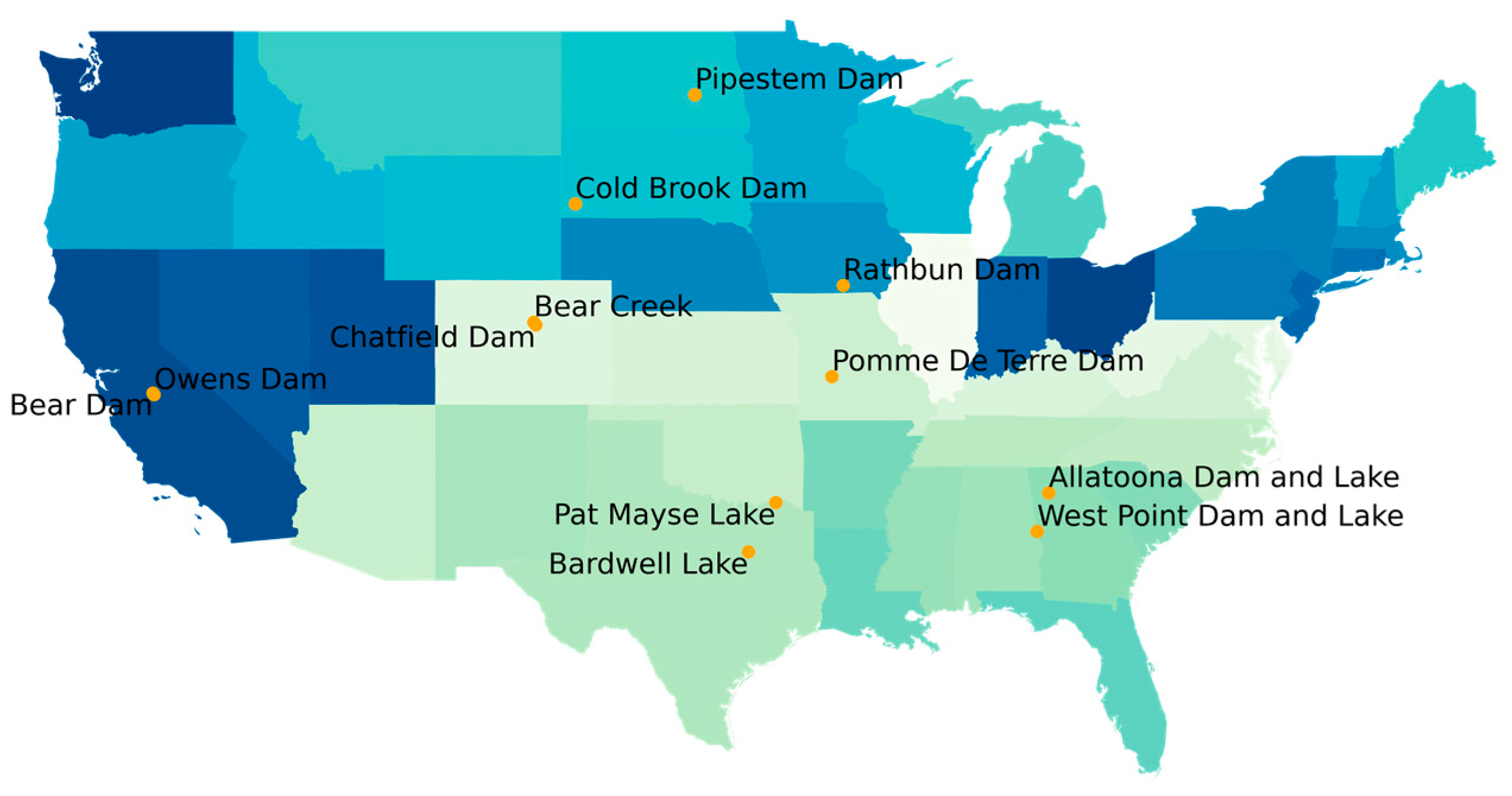
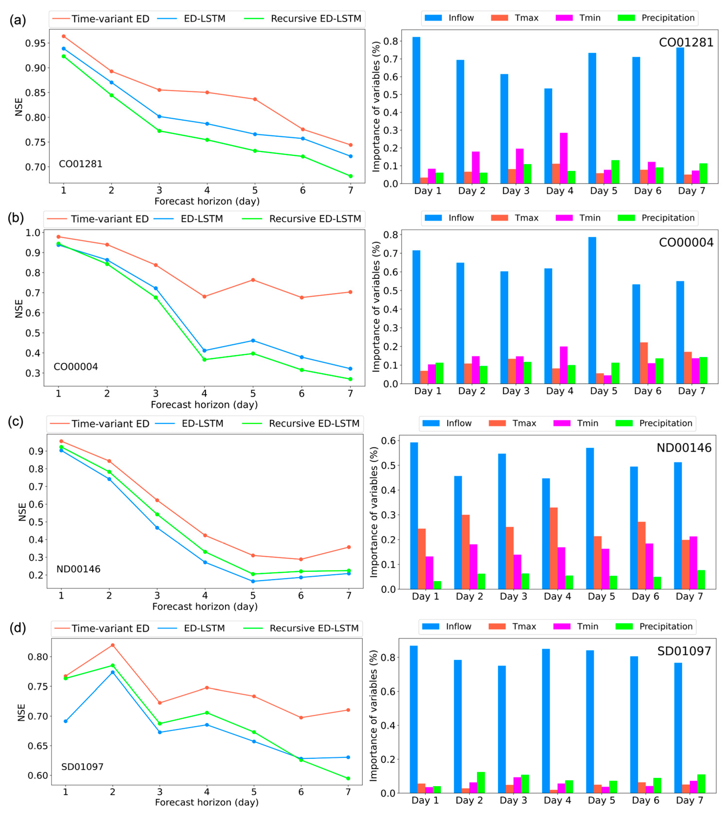
The time-variant ED model was applied to predict 7-day ahead inflows for four reservoirs located in Colorado, North Dakota, and South Dakota, and its performance was compared against the ED-LSTM and recursive ED-LSTM models. As illustrated in Figure 5, the results indicate that the time-variant ED model consistently outperforms both benchmarks across all forecast horizons. Although forecasting accuracy decreases with increasing lead time, the time-variant ED model mitigates this decline more effectively than the ED-LSTM and recursive ED-LSTM models. The superior performance of the time-variant ED model can be attributed to its dynamic encoding mechanism, which adjusts the model’s parameters for each forecast horizon. This flexibility enables the model to better capture time-varying dependencies between historical inputs and future inflows. In contrast, both the ED-LSTM and recursive ED-LSTM models rely on a fixed encoder structure, which may struggle to adapt to the evolving patterns of inflow over different forecast horizons.

The developed EB-IG method was applied to analyze the relative importance of input variables in the forecast models, providing insights into the underlying drivers of inflow dynamics. As shown in Figure 5, historical inflow consistently emerges as the dominant factor influencing inflow predictions across all reservoirs, accounting for more than 50% of the total importance. This strong dependence on past inflows is expected, given that a substantial portion of the inflow in these regions is driven by snowmelt, which tends to create more stable and predictable inflow patterns. Temperature ranks as the second most important variable. Its importance can be attributed to its role in regulating the timing and intensity of snowmelt, especially during spring and summer when snowmelt is most significant. Precipitation ranks as the least important factor. Its effects are more immediate but transient, as rainfall contributes less to overall inflow compared to the cumulative and more sustained impact of snowmelt in these regions. To conclude, our analysis reveals that these reservoirs are characterized by relatively stable inflow patterns, with historical inflow data playing a crucial role in understanding and predicting future inflows.

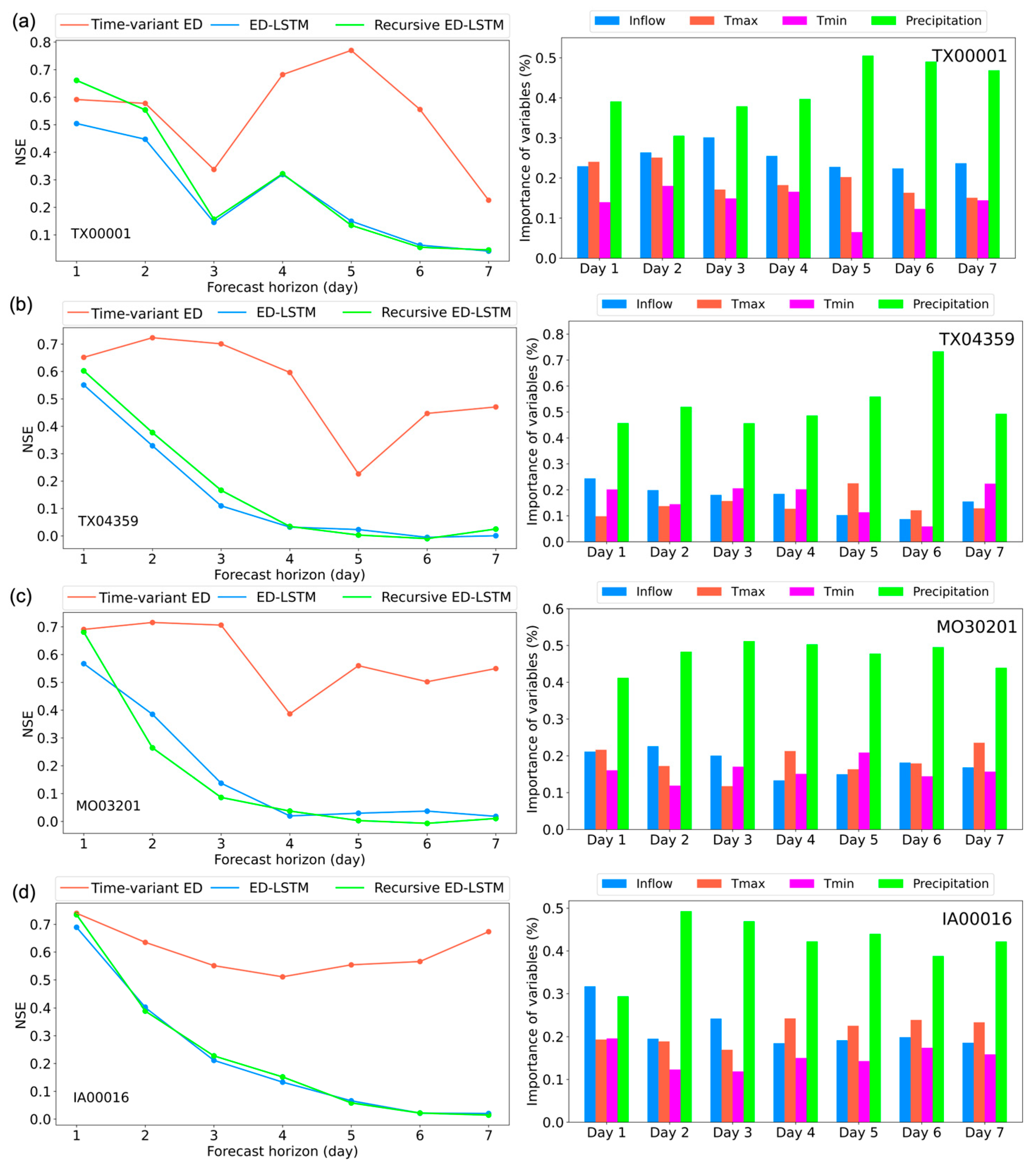
Figure 6 illustrates the results for two reservoirs in Texas, one in Missouri, and one in Iowa. The developed time-variant ED model significantly outperforms both the ED-LSTM and recursive ED-LSTM models, particularly at longer forecast horizons. Both benchmark models exhibit a notable decline in accuracy after the 2-day forecast horizon, falling into the category of “Unsatisfactory”. This sharp decline in performance highlights the limitations of fixed encoder structures in capturing the time-varying dynamics of inflow, especially for longer forecast horizons. In contrast, the time-variant ED model, with its adaptive ED architecture, shows a much more gradual decline in performance, effectively mitigating forecast degradation over longer horizons.

The variable importance analysis in Figure 6 reveals that precipitation is the primary driver of inflow in these regions. Unlike the snow-dominated reservoirs in Colorado and the Dakotas, the inflow dynamics in Texas, Missouri, and Iowa are largely influenced by rainfall events. Consequently, precipitation plays a critical role in shaping inflow patterns, with its immediate and substantial impact making it the most significant factor driving forecast accuracy for these reservoirs. This insight suggests that water resource managers in these regions should prioritize short-term precipitation forecasts in their decision-making processes.

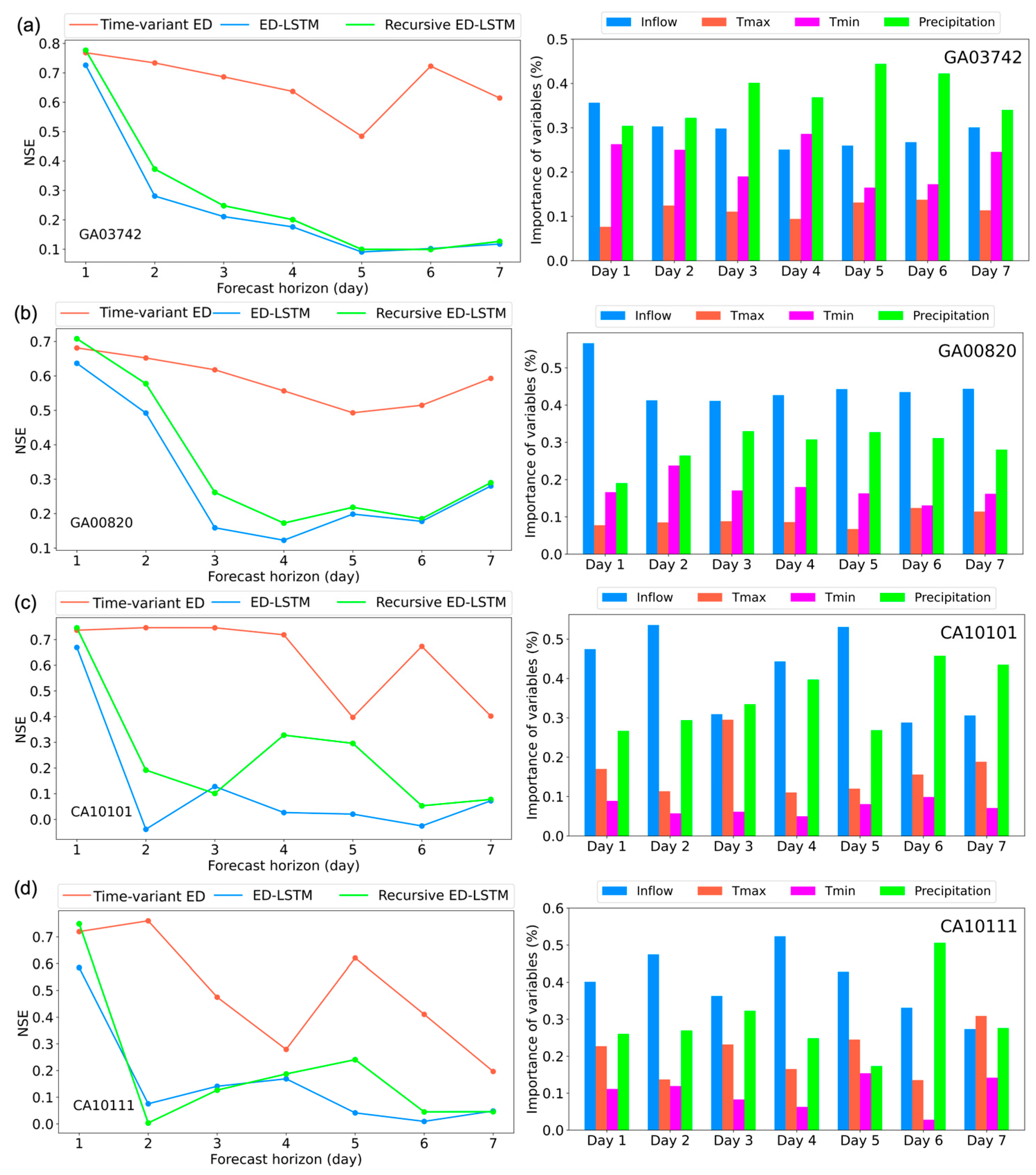
Figure 7 presents the results for two reservoirs in Georgia and two in California. The time-variant ED model significantly outperforms both the ED-LSTM and recursive ED-LSTM models, particularly at extended forecast horizons. In Georgia, the time-variant ED model maintains “Good” performance across all 7 days, while both benchmark models fall below the “Unsatisfactory” threshold after day 2. In California, the performance gap is even more pronounced, with benchmark models dropping into the “Unsatisfactory” category after just 1 day. These results highlight the effectiveness of the time-variant ED model in capturing the time-varying temporal dependencies, mitigating the forecast degradation observed in the benchmark models over extended horizons.

The variable importance analysis in Figure 7 reveals that both historical inflow and precipitation are the primary drivers of inflow in Georgia and California. In Georgia, both precipitation and the historical inflow are crucial for capturing inflow patterns. This balanced influence indicates the importance of both recent meteorological events and longer-term hydrological trends in shaping reservoir inflows. In California, the analysis shows a slight predominance of historical inflow influence, which aligns with the state’s seasonal and often drier climate. Here, historical inflow captures the baseline flow patterns that persist through dry periods. However, precipitation remains a key factor, particularly during wet seasons or storm events. This analysis demonstrates that accurate inflow forecasts in both regions rely heavily on the interplay between past inflow trends and current precipitation patterns, reflecting the complex and dynamic nature of regional hydrology.

For each of the reservoirs, the time-variant ED model consistently outperforms the ED-LSTM and recursive ED-LSTM models, particularly over extended forecast horizons, as evidenced by the NSE scores. The adaptive nature of the time-variant ED model allows it to maintain a more gradual reduction in performance. Overall, the time-variant ED model’s ability to capture time-varying dynamics makes it a more reliable tool for multi-step ahead inflow forecasting across diverse hydrometeorological conditions. This improved forecasting capability, coupled with insights from the variable importance analysis, can help reservoir operators make more informed decisions, optimize water management strategies, and better prepare for flood or drought scenarios.

5. Discussions

To better understand the performance differences among the studied forecasting models—ED-LSTM, recursive ED-LSTM, and the proposed time-variant ED model—we summarize their respective advantages and limitations. The standard ED-LSTM offers a clean, straightforward design with fixed parameters across all forecast horizons. This consistency makes it easy to implement and generally stable in performance. However, its main drawback is that the encoder remains static, lacking the flexibility to adjust to evolving hydrometeorological conditions across different lead times. The recursive ED-LSTM model improves upon this by allowing long-range prediction through feeding each prediction back as input for the next step. While this design supports extended forecasting, it is prone to recursive error propagation, which can significantly compromise performance at longer lead times due to the compounding of inaccuracies. In contrast, our time-variant ED model introduces a dynamic encoder mechanism that adapts its parameters at each forecast step based on current inputs. This structure enhances the model’s ability to handle input shifts across time. Consequently, it improves forecasting accuracy, particularly at mid-to-late horizons where conventional models typically struggle. The primary trade-offs of this approach include increased model complexity, higher computational demands, and the need for careful training to ensure stable convergence. In addition, it is worth noting that while our sequential train-test split demonstrates performance on unseen data, future work should include systematic temporal validation (e.g., seasonal holdout or cross-year validation) to assess model robustness more rigorously across varying hydrological conditions and long-term trends.

One observation from our results is the variability in multi-step inflow forecasting accuracy across different forecast horizons. In theory, the predictive skill of a dynamical system tends to degrade as the forecast lead time increases. This degradation is often caused by the gradual loss of system memory, where the effects from the initial states diminish, and the external forcings become increasingly uncertain. However, ML model performance is heavily dependent on the training data and the patterns learned, which means these models do not always follow a consistent decline trend across all forecast horizons. Certain horizons may be easier to predict due to more stable dynamics, while others present more challenges due to greater uncertainty or complexity.

To explore the variability in forecast performance across different horizons, we conduct an interpretative analysis focusing on two reservoirs. In Reservoir CA10101, prediction accuracy fluctuates at certain horizons, notably dipping at the fifth forecast horizon before improving at the sixth, as shown in Figure 7c. These fluctuations align with shifts in the importance of key variables. Between the fifth and sixth horizons, the significance of inflow decreases while the influence of precipitation increases. Since inflow forecasts rely on prior predictions, high importance of this inflow variable can propagate errors, negatively impacting accuracy. The model’s performance improves when inflow’s weight decreases, as observed at the sixth horizon. A similar trend was observed for Reservoir TX00001, as shown in Figure 6a. Forecast accuracy improves steadily from the third to the fifth horizon before declining at the sixth. This shift corresponds to the variable importance analysis, which reveals a growing influence of precipitation, peaking at the fifth horizon and decreasing at the sixth. These results highlight how changes in the importance of key variables can affect forecast accuracy across different horizons. In particular, the counterintuitive improvement in mid-to-late horizon forecasts is attributed to the model’s time-variant encoder, which adaptively shifts reliance from autoregressive inflow to more informative external drivers like precipitation, thereby mitigating error accumulation.

For future improvements, incorporating multiple meteorological forcing products presents a promising opportunity to enhance model accuracy [32]. These products provide complementary information on crucial variables such as precipitation and temperature, which influence inflow dynamics differently across regions and seasons [10]. Leveraging this diverse data could lead to more robust inflow predictions that account for a wider range of hydroclimatic conditions. The primary challenge lies in effectively integrating these diverse forcing products into a unified forecasting model. Our future work will focus on restructuring the model to enable adaptive weighting of these inputs. For instance, implementing attention mechanisms will allow the model to dynamically assign importance to different meteorological products based on their relevance to specific forecast horizons. In addition, we will apply these modifications to explore the application of these methods to all major reservoirs across the US, which will expand the model’s applicability to diverse hydrometeorological conditions.

6. Conclusions

In this study, we developed a time-variant ED model for enhanced multi-step inflow forecasting, capable of predicting reservoir inflows up to seven days ahead. Our approach addresses key limitations in conventional models such as ED-LSTM and recursive ED-LSTM, which rely on static encoder parameters. By incorporating an adaptive encoder structure that dynamically adjusts parameters based on evolving hydrometeorological inputs, our time-variant ED model adapts better to changing conditions, leading to more accurate and reliable inflow forecasts. Another contribution of this work is the development of the EB-IG method for variable importance analysis. By introducing multiple baselines randomly sampled from the training data, this method provides a more comprehensive assessment of factors that significantly influence inflow forecasts under diverse hydrometeorological conditions.

Our results demonstrate that the time-variant ED model outperforms traditional methods in multi-step inflow forecasting, particularly at longer lead times where conventional models typically struggle. The model’s adaptive capacity helps improve forecasting accuracy across all forecast horizons, providing reservoir operators with more accurate predictions. Furthermore, the enhanced variable importance analysis reveals valuable insights into the dominant drivers of inflow at various reservoirs. By identifying key factors such as historical inflow and precipitation, our research offers reservoir operators a deeper understanding of the complex dynamics influencing inflow patterns.

The developed time-variant ED model demonstrates significant potential for advancing multi-step inflow forecasting in complex hydrological systems through adaptive ED approaches. This methodology enhances prediction accuracy and model flexibility, effectively addressing challenges posed by dynamic hydroclimatic conditions. By integrating multiple data sources with adaptive weighting mechanisms, as proposed for future work, we can develop more robust and reliable forecasting models. These advancements have broad implications for reservoir management, including enhanced operational efficiency, optimized water resource allocation, and improved preparedness for flood and drought events.

Importantly, the improved multi-step forecasts generated by our time-variant ED model have direct implications for reservoir operations. In particular, these forecasts can be integrated into dispatch planning tools, such as dispatcher graphs or reservoir rule curves, to inform real-time decision-making on water release, storage regulation, and flood control. In future work, coupling our forecasting system with optimization algorithms or simulation-based reservoir operation models offers a promising direction to develop adaptive, data-driven dispatch plans. This synergy between advanced inflow forecasting and operational planning represents a promising path toward data-driven, climate-resilient water resource management.