Reservoir Basin-Scale Landslide Susceptibility Assessment by Machine Learning Techniques: A Case Study of San Pietro Dam, Southern Italy

Abstract

Research on landslides around reservoirs is necessitated to strengthen risk prevention and mitigation, as their occurrence has catastrophic consequences. For reservoir safety assessments, landslide susceptibility analysis is commonly concentrated on single reservoir bank slopes or individual landslides. However, focusing solely on bank slopes and individual landslides gives an incomplete picture of how safe the reservoir is from possible landslide related risks, since landslides from distant slopes can also adversely affect the reservoir in different ways. In this paper, landslide susceptibility assessment was conducted using machine learning models (Gradient Boosting Machine, XGBoost, Random Forest and Ensemble Stacking) in the area around the San Pietro Dam, an earth dam located in Southern Italy, in a region highly prone to landslide hazards. The landslide inventory for the area was used to generate landslide and non-landslide points for model training and testing. The area under curve (AUC) of a receiver operating characteristic (ROC) curve approach was used to evaluate, validate, and compare the performance of the four models. Results indicated that the ROC AUC values of the models ranged from 0.76 to 0.77, with the Random Forest, Gradient Boosting and Ensemble stacking models having AUC values of 0.77. All the models classified about 15–20% of the reservoir basin as highly susceptible to landslides. The generated basin-scale landslide susceptibility maps can be used to prioritize monitoring and maintenance in areas around the dam that have been identified as highly susceptible.

1. Introduction

Reservoirs are an important infrastructure that play vital roles, including supplying drinking water, generating hydroelectric power, storing and supplying water for irrigation, providing recreational opportunities, and flood control. Due to population growth and urban expansion, the number of dams built for water storage worldwide is increasing to meet the growing demand from towns, agriculture, industry and hydropower generation. One of the fundamental activities in reservoir management is hazard identification and assessment, which informs the implementation of necessary mitigation strategies and facilitates the formulation of adequate safety measures and emergency plans to ensure the sustainability of the reservoir and its surrounding environment [1].

Landslide hazards can hinder the sustainable management of reservoirs, especially those which are located in mountainous terranes. Landslide-related hazards can occur in both natural and artificial reservoir environments. They cause an influx of collapsed soil and rock masses into reservoirs, which consequently accelerates sedimentation and, as a result, irreversibly reduces storage capacity, thereby compromising the core hydrological functions of the reservoir [2,3]. Furthermore, in the event of landslide occurrence, cascading events can occur, including upstream backwater formation, flooding in downstream areas, changes in riverbed dynamics, and secondary landslides may be triggered [4]. Understanding landslide risk in reservoir environments cannot be overstated, as history shows that these events, in various parts of the world, can result in significant, catastrophic consequences in both upstream and downstream areas [5,6,7,8]. An ill-famed example is the landslide disaster that occurred within the Vaiont Dam reservoir (northeastern Italy) on 9 October 1963 [9]. Continuous advancement of landslide hazard assessment in reservoir areas is needed due to the ongoing climate change and rapid population growth, which can significantly exacerbate the impacts of hydrometeorological natural hazards on reservoir slopes [10,11].

Landslide hazard predictions and monitoring are crucial measures to reduce the damage and losses caused by landslides to infrastructure such as dams. Landslide monitoring and assessment also provide a basis for operational early-warning systems for potential slope-failure hazards [12]. This is essential, since the safety of infrastructure also means the territories in which they are located can also be considered safe from their associated risks [13]. One of the most effective traditional approaches to landslide prediction is landslide susceptibility analysis, which aims to generate landslide susceptibility maps that portray the degree of the spatial probability of landslide occurrence in a specific area based on local terrain characteristics [14]. This information is essential for territorial administrators to assess potential landslide events and their consequences, prioritise mitigation measures, implement early warning systems, and ultimately reduce risk. The main assumption in most landslide susceptibility assessment studies, especially those using statistical methods, is that the past is the key to the present [15]; hence, landslides are believed to occur throughout a study area when the same landslide predisposing and triggering factor combinations exist [14,15,16].

Approaches for assessing landslide susceptibility can be broadly classified into qualitative and quantitative methods [17,18,19]. Qualitative methods include a number of techniques, such as the geomorphological analysis [19,20,21,22,23]; landslide inventory analysis [24,25]; and expert analysis [26,27,28]. These methods are largely based on the expert’s knowledge and experience in assessing landslide potential; hence, they tend to be subjective, so the corresponding results cannot be replicated even with the same input data [15,20]. Quantitative methods, on the other hand, are mainly composed of statistical techniques [29,30,31]; probabilistic techniques [32,33]; and physically-based numerical modelling techniques [34,35,36,37,38]. These techniques are nowadays commonly used for landslide susceptibility mapping, as they are based on real data and interpretations, thereby overcoming the subjectivity that is generally associated with qualitative approaches.

Lately, various landslide susceptibility models evolving from statistical methods have been employed within machine learning (ML) approaches to generate more accurate landslide susceptibility zonation [39]. These ML algorithms basically learn from data without depending on rule-based functions [39]. Several ML approaches for assessing landslide susceptibility are now available, including artificial neural network (ANN)-based models [39,40,41,42]; decision tree-based models such as random forests and extreme gradient boosting (XGBoost) [39,43,44,45]; and support vector machines [46,47,48]. Ado et al. [49] provide a comprehensive review of ML approaches. These approaches are preferred over traditional statistical methods because they are more tolerant of noisy or imbalanced data, a common problem in most existing landslide inventories [50].

Reservoir environments have peculiar characteristics, since the occurrence of landslides in reservoir areas may be influenced by reservoir operations. For instance, due to both impoundment and reservoir operations, more than 5300 landslides were reported around the Three Gorges Dam [51,52]. Jones et al. [53] found that about half of the landslides surrounding the Grand Coulee Dam from the year 1941 to 1953 occurred during reservoir filling operations and about 30% during reservoir drawdown operations. These studies clearly indicate that the effects of impounding-drawdown operation cycles on slope stability behaviour depend on conditioning factors such as slope geometry, drawdown rate, soil material properties, initial pore-water pressure distribution, as well as the reservoir water levels at the beginning and end of operation. Hence, there is a need to understand landslide hazards under different operating conditions [54].

Despite periodic landslide susceptibility assessments and the implementation of related mitigation interventions in water reservoirs, most existing studies and management practices focus on specific slopes or individual landslides at the scale of a single reservoir bank slope [7,55,56,57,58,59]. However, assessing slope stability at the scale of a single bank slope provides a partial view of the landslide hazard conditions around the reservoir. In this perspective, ML approaches for landslide susceptibility assessment are well established, and their strengths and limitations are well documented in the literature. However, their applications to reservoir basins for landslide risk management are scarce. Therefore, in this paper, four ML models were used to assess landslide susceptibility in the area around the San Pietro Dam, which is located in the Campania region, Southern Italy. Such a catchment-wide landslide susceptibility assessment is here believed to be essential for proactive hazard management, reservoir operation planning, as well as the long-term sustainability and safety of the reservoir system. The outcomes of this study are expected to be useful for identifying areas that are susceptible to landslides with high accuracy, thereby likely to be affected by landslides. Thus, allowing the selection of suitable targets for detailed investigations, using, for example, high-resolution slope-scale numerical models, and landside mitigation or risk management activities by decision-makers.

2. Materials and Methods

2.1. Study Area

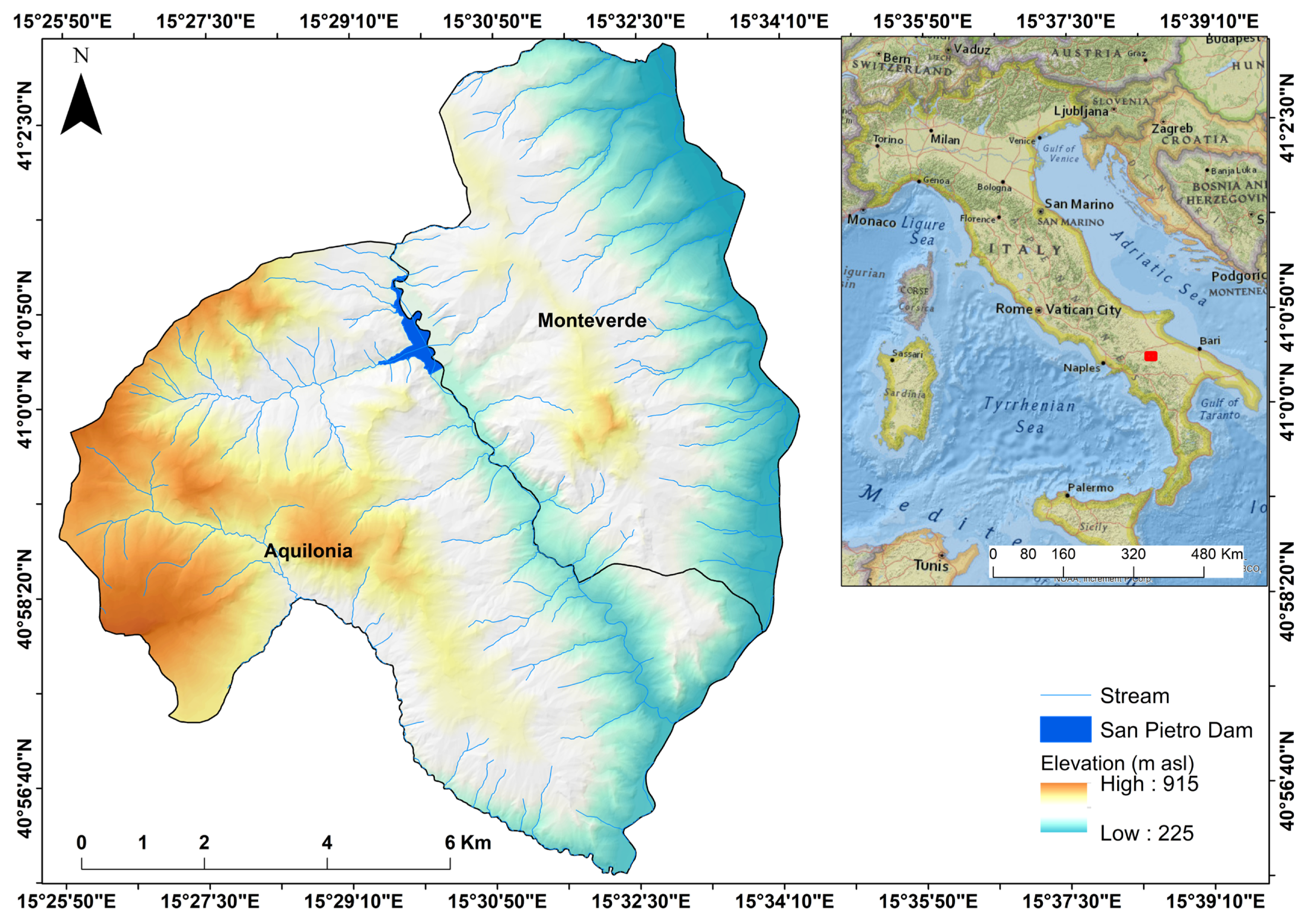
The study area, which is a basin of the San Pietro Dam covering about 95 Km², lies between two small towns of Aquilonia and Monteverde, both located in the Campania Region, Southern Italy (Figure 1). Generally, the study area experiences a temperate Mediterranean-type climate, largely influenced by Tyrrhenian-origin humid air masses [60]. Winters are cool and rainy, with temperatures that rarely drop below 0 °C, except in the uppermost areas of the mountains, where the temperature can drop below 0 °C and snowfall is frequent. The summer is generally hot and dry, with average temperatures around 25 °C.

The geomorphological context of the study area is characterized by a variety of landscapes, mainly composed of hilly landforms with gentle slopes and wide watersheds [61]. As part of the Southern Apennine orogenic chain, the study area is characterized by complex tectonic activity related to the convergence of the European and African tectonic plates along a west-directed subduction zone [62,63]. The study area possesses a complex, hilly and mountainous orography, which makes it prone to various landsliding processes [64]. Precisely, the area is situated at the external border of the calcareous Southern Apennines, in a structural depression filled with Pliocene deposits and overlaid by Quaternary formations [65]. The area is composed of numerous structures and diverse lithologies belonging to different units. The oldest outcrops of the area, primarily consist of clay-sandy and marly layers in the upper sections, while the lower sections feature denser marly-carbonate and siliceous formations, all of which are part of the Meso-Cenozoic basin sequences [65]. An unconformity separates the aforementioned deposits from coarse-grained sandstone and polygenic conglomerate-dominated flysch deposits, which belong to the Irpinian Supersynthem [66].

2.2. Landslides Inventory

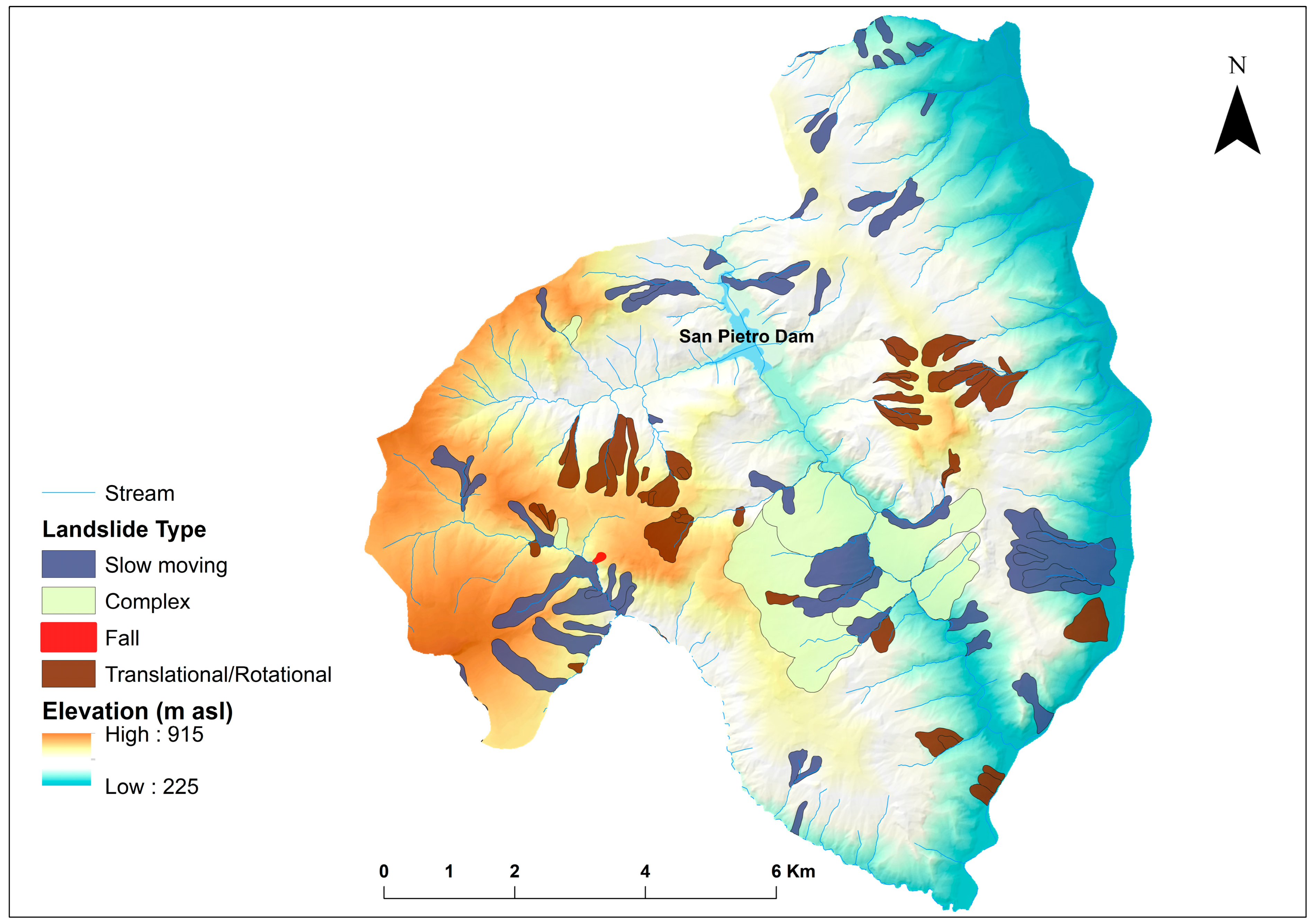
The landslide inventory map (Figure 2) used as the reference map for the susceptibility analysis presented in this work was obtained from the Italian Landslide Inventory (IFFI Project). This inventory was developed since 2005 by the Italian National Institute for Environmental Protection and Research (ISPRA) in collaboration with 21 Regions and self-governing Provinces of Italy, following a common landslide mapping procedure [67]. Field surveys, searching in historical documents, interpretation of aerial photos, and GIS mapping were the main methodologies that were used to generate the inventory. The mapping scale of the inventory is 1:10,000 in most of Italian territory and 1:25,000 for the mountainous and sparsely populated areas. For the area in the current study, there are about 115 landslides, of which 50% of them are classified as slow-moving landslides, 43% as rotational/translational slides, and the rest as complex slides.

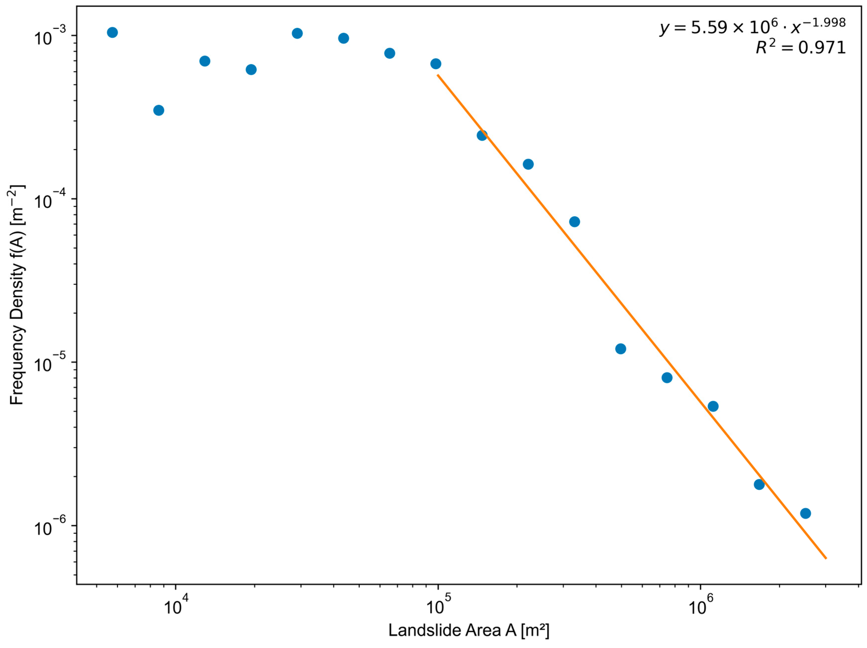
Completeness and resolution are fundamental concepts to be considered when using a landslide inventory [68,69]. Completeness is the extent to which the actual distribution of landslides is portrayed by an inventory, while resolution is the smallest landslide area consistently recognised and mapped or recorded in an inventory [68]. In this research, we utilized the approach suggested by Malamud et al. [70], to assess the completeness of the inventory, operating under the premise that a complete inventory ought to exhibit a power-law correlation across a broad spectrum of orders of magnitude. In this approach, the position of the roll-over point of an inventory can be observed. For landslide sizes smaller than the rollover point, the inventory is considered to reduce these events, with fewer occurrences recorded than expected under the power-law distribution. Figure 3 shows the calculated power law for the study area landslide inventory, along with the correlation coefficient, which is about 0.97. The landslide areas extend from approximately 3 × 10⁴ m² to 3 × 10⁶ m². In particular, the rollover is observed for landslides with an area smaller than 10⁵ m². Based on the reasonably high observed correlation coefficient, the inventory is considered complete for landslides larger than the roll-over point. The slope of the power law tail is about 1.998. As can be observed, the resolution, or landslide area consistently mapped, is below this rollover. In general, the inventory completeness is acceptable and sufficient for further analysis of landslide patterns in the area.

In this work, the landslide inventory map was used as the basis for generating data for modelling landslide susceptibility in the study area. Within the landslide polygons, 208 random landslide points were sampled, and 205 non-landslide points were sampled, yielding a total of 413 points. To prevent model bias, balanced sampling between landslides and non-landslide points was preferred. This relatively small sample size was limited by the number of landslides in the available inventory, as sampling several points within the same landslide polygon could introduce spatial autocorrelation. The implication for this limited sample size is that the models may be overfitted. The non-landslide points were sampled so that they are at least 50 m away from the landslide shown on the inventory map. The buffer distance was iteratively chosen, and a 50 m distance was recognized to enable some stable pixels close to the dam to be selected as well, so that models are properly trained.

2.3. Landslide Conditioning Factors

To investigate landslide susceptibility in the study area, a set of conditioning factors was selected. Landslides typically result from the combined influence of topographic, geological, hydrological, and anthropogenic factors [71]. The selection of the conditioning factors was mainly based on available knowledge of the landslide initiation process in the study area, the geo-hydrological nature of the study area and the availability of data [14,18,71]. A total of eleven parameters were selected, including slope steepness, elevation, aspect, curvature, topographic position index (TPI), topographic wetness index (TWI), lithology, soil texture, land cover, distance to roads and distance to streams. Topographic parameters like slope steepness, slope aspect and elevation were derived from a Digital Elevation Model (DEM) with a resolution of 10 m that was downloaded from the Tinitaly DEM website [72]. The DEM was created using a Triangular Irregular Network (TIN) with the following elevation data inputs: contour lines and spot heights sourced from the Italian Regional topographic maps, satellite-based GPS points, as well as data from ground-based and radar altimetry measurements [72]. Thematic layers were acquired from different sources, with the data varying in generalisation and scale. Therefore, the datasets were resampled to a 10-m raster cell resolution to conform with the digital elevation model used.

2.3.1. Slope Steepness

Slope steepness is a very important parameter for landslide studies, because it has a direct relation with the occurrence of landslides, as it has complete control over the movement of materials based on gravity [73]. As a result, this factor is often used in generating landslide susceptibility maps. It is common knowledge that landslides are more frequent on steeper slopes due to gravity stress than on gentle slopes [74]. The slope map was generated from the 10 m resolution DEM.

2.3.2. Aspect

Aspect denotes the direction of slope, usually expressed in degrees ranging from 0° to 360 [75]. Orientation of a slope is considered an important factor in landslide susceptibility studies since it affects the slope’s exposure to sunlight, wind direction, degree of saturation due to rainfall and discontinuity conditions [76,77,78]. A slope aspect map was generated from the DEM data and then divided into the following 9 classes, including the flat class, and 8 direction-based classes, namely: north, northeast, east, southeast, south, southwest, west, and northwest [76].

2.3.3. Elevation

Elevation is a significant landslide conditioning factor because geomorphological and geological processes are influenced by it. Elevation affects topographic characteristics, which contribute to spatial variations in many landform processes and vegetation distribution [79]. Furthermore, elevation influences climate in terms of the amount, intensity, and distribution of rainfall that an area receives, which also affects landsliding processes [79]. Elevation of the area was obtained from the 10 m resolution DEM, ranging from 225 m to 915 m above sea level.

2.3.4. Topographic Position Index

The topographic position index (TPI) quantifies the relative position of a cell in a landscape; it is calculated using a DEM as the elevation difference of each DEM cell from the mean elevation of a specified neighbourhood around that particular cell, with the radius of the neighbourhood specified beforehand [80]. Since TPI shows the difference between the elevation of a point and its surroundings, low values signify that a cell is lower than its immediate surrounding terrain, which possibly implies a higher odds of landslide occurrence when accompanied by other relevant conditioning factors [81].

2.3.5. Topographic Wetness Index

The topographic wetness index (TWI), which is calculated as the logarithm of the upstream area divided by slope, is used to evaluate the static soil moisture content [82]. TWI indicates the level of saturation or wetness due to the soil water content along a slope [83]. Thus, a high TWI value indicates a high amount of water content stored in the slope material, which can affect slope instability [81,82].

2.3.6. Landcover

According to Glade [83], land use and land cover changes caused by human activities like deforestation, intensive agriculture, and farming on steep slopes can trigger slope instability. Vegetation makes a significant contribution to the resistance of slope movements. Vegetation with a well-developed root network enhances the shear resistance of the slope material [84]. This is accomplished through the natural anchoring of materials on the slope. Furthermore, it lessens erosion and enhances the stability of the slope. Conversely, slopes that are bare or are partially vegetated tend to be more vulnerable to erosion and, as a result, are at a higher risk for slope instability [85].

The landcover map was obtained from the Coordination of Information on the Environment (CORINE) program portal [86]. The CORINE is one of the most relevant and readily available landcover datasets in the European context [87]. The data used were for the 2021 reference year, which shows the dominant land cover among eleven basic land cover classes for each pixel at a resolution of 10 m. For this study, five land-cover classes were generated. All urbanised areas, including road and rail networks, industrial, commercial, and residential areas, were grouped into a single class termed ‘‘Built up areas”. Other land cover classes included water bodies, forests, grasslands, and shrubs.

2.3.7. Lithology

Various rock types differ in composition and structure, which, in turn, affect permeability and strength properties and, consequently, slope stability in a positive or negative way. High-strength rock masses are less susceptible to failure [88]. The lithological map of the study area was derived from an existing provincial 50 k-scale geological map, prepared by the Italian Geological Survey. The geology of the study area was reclassified into four dominant lithological units, namely: Delta and floodplain deposits; Pelitic sands and conglomerates with olistostromas; Marly limestones, marl, pelites, sandstone, conglomerate, and gypsum; and Marl, pelites, sandstone, and conglomerates.

2.3.8. Soil Texture

There exists a close relationship between soils and landslides, especially shallow ones, hence different soil property maps are used as predictor factors for landslide occurrence [89]. In this study, soil type was used as one of the conditioning factors for landslide occurrence. The soil map was obtained from the Geoportal for the Territorial Information System of the Campania Region, available as a vector map, and was reclassified into three dominant soil classes: clay and marly soils, arenaceous (sandy) soils, and river-channel alluvial soils.

2.3.9. Curvature

Curvature is mathematically defined as the change in slope angle along a very small arc of a curve, which simply describes how the shape of the terrain surface bends or changes [90]. The shape of the slope plays a role in landslide conditioning. In particular, landslides may be concentrated in concave curvature slopes due to the concentration of water in these slopes, which increases the degree of saturation in a slope [40]. The curvature map of the study area was prepared from the 10 m resolution DEM. In this study, total curvature (the combination of plan and profile curvature) was used as one of the inputs to assess landslide susceptibility in the study area.

2.3.10. Distance from Streams

Proximity to streams is another factor which can also influence the occurrence of landslides in an area. Through toe erosion and saturation of the slope materials, active stream incision can significantly affect slope instability by steepening the slope further and producing a high degree of slope saturation [91]. A map showing the distance to the stream for every pixel in the study area was derived from the stream map, which included main streams in the area. The map of the distance from streams was generated by Euclidean distance ring buffering.

2.3.11. Distance from Roads

Distance from roads is described as one of the anthropogenic factors that influences the occurrence of landslides. Construction of roads significantly lowers the stability of the crossed slopes due to the removal of slope support, and increases the micro topography generated in the process of slope excavation, thereby accelerating the likelihood of landslides occurring in the affected slopes [44,91]. Furthermore, these anthropogenic activities can block natural drainage. The map showing the distance to roads was derived from the roads map of the study area, which primarily included national and local roads. The distance-from-roads map was generated using Euclidean distance ring buffering.

2.4. Landslide Conditioning Factors Correlation Analysis

Good-quality input data is a prerequisite for achieving reliable results from a landslide susceptibility model [92]. High correlations among used landslide conditioning factors can lead to unstable model coefficients, eventually making it difficult to interpret the influence of an individual factor on landslide occurrence [92,93]. Removing highly correlated or collinear variables is therefore advantageous, as it improves model performance, reduces standard error, and enhances the stability of machine learning models [94]. The associations between the eleven landslide conditioning factors utilized in this study to evaluate landslide susceptibility were examined using the Pearson correlation coefficient approach. The degree of linear correlation between two variables can be represented by the Pearson correlation coefficient (PCC), which ranges from −1 to 1. PCC values less than 0.3 indicate weak correlation, values between 0.3 and 0.7 indicate moderate correlation, values between 0.7 and 0.9 indicate strong correlation, and values greater than 0.9 indicate very strong correlation [93,95]. PCC was computed among the factors using Equation (1). Despite notable limitations, such as its inability to adequately capture nonlinear relationships and its poor handling of categorical variables, PCC was used as an exploratory tool to assess whether strong linear relationships exist among the landslide conditioning factors.

$$PCC={\displaystyle \frac{n\sum {\mathcal{X}}_i{\mathcal{Y}}_i-\sum {\mathcal{X}}_i\sum {\mathcal{Y}}_i}{\sqrt{(n\sum {\mathcal{X}}_i^2-(\sum {\mathcal{X}}_i{)}^2\left)\right(n\sum {\mathcal{Y}}_i^2-\left(\sum {\mathcal{Y}}_i{)}^2\right)}}}$$

(1)

where $n$ is the sample size; $𝒳$_i is the i-th value of variable $𝒳$ and $𝒴$_i is the i-th value of variable Y.

2.5. Approaches for Landslide Susceptibility Analysis

Four machine learning algorithms, namely Random Forest, Gradient Boosting Machine, Extreme Gradient Boosting, and Ensemble Stacking, were selected to assess the susceptibility to landslides around the San Pietro Dam. These algorithms are widely used in landslide susceptibility studies and have proven to have sufficient accuracy [46,96,97,98].

2.5.1. Random Forest

The Random Forest (RF) algorithm is basically an ensemble machine learning technique that is commonly used for purposes of classification and regression [99]. In this study, the RF model was applied as an ensemble of decision trees to identify any possible occurrence of non-linear relationships between landslide phenomena and landslide predisposing factors, while minimising overfitting via bootstrap aggregation [98]. Predictor variables derived from multi-source raster layers were standardised where necessary, whereas categorical variables, including land cover, lithology, and soil texture, were maintained in their original categories.

2.5.2. Gradient Boosting Machine

Originally derived by Friedman [100], the Gradient Boosting Machine (GBM) algorithm is an ensemble machine learning method that iteratively improves its predictive performance through the identification of deficiencies in previous model runs and modification of these in subsequent predictions [101,102,103,104]. This iterative process helps to improve the model to enhance the accuracy of its predictions by mitigating the errors of preceding models through the process of learning from the residuals, which is particularly relevant for unbalanced landslide datasets [104,105,106].

2.5.3. Extreme Gradient Boosting

The Extreme Gradient Boosting (XGBoost) method is an effective machine learning technique that combines several decision tree models to create a more powerful classifier, which is improved by gradient boosting decision [96,107]. The fundamental idea of this algorithm is to fit the residual of the prior prediction by learning a new function each time, thereby determining the score associated with each node based on the sample attributes. XGBoost was implemented as a regularised gradient boosting framework designed for high predictive performance and robustness. The model leverages second-order gradient information and built-in regularisation to control model complexity and mitigate overfitting [96].

2.5.4. Ensemble Stacking

Finally, the ensemble stacking technique was used to combine the aforementioned three machine learning models to produce a susceptibility prediction, compensating for the limitations or biases of individual algorithms [49,108]. In this study, the stacking approach was implemented to integrate the complementary strengths of the aforementioned base models. In this framework, optimised base learners were combined, and their probabilistic outputs were used as inputs to a logistic regression meta-learner, which learned the optimal weighting scheme for final prediction.

All models were subjected to hyperparameter optimisation using Bayesian optimisation via BayesSearchCV from scikit-optimise, implemented within the scikit-learn framework. Bayesian optimisation constructs a surrogate probabilistic model of the objective function and sequentially selects hyperparameter configurations by maximising an acquisition function, thereby improving search efficiency in high-dimensional spaces [107]. This approach was preferred as it is helpful for environmental susceptibility modelling with limited sample sizes, as in this case study, wherein overfitting risk may be amplified as a result of exhaustive search, which increases variance in performance estimates [44]. For the RF model, tuned parameters included the number of trees (100–500), maximum tree depth (3–20), and minimum samples required for node splitting (2–10). For boosting-based models, the number of estimators (100–500), maximum tree depth (3–10), and learning rate were optimised.

2.6. Evaluation Metrics for the Models

Validating a model’s performance is essential for landslide susceptibility mapping activities so that the outcomes can be reliably utilized for risk reduction and hazard mitigation decision-making purposes [109,110]. Therefore, proper evaluation of the quality of a landslide susceptibility map requires more sophisticated solutions, as this will support subsequent uses to which the derived susceptibility results can be used for [111]. Validation of the model results was performed using stratified 5-fold cross-validation. This was implemented using the stratified k-fold function in scikit-learn. While preserving the proportion of positive and negative landslide samples within each fold, the dataset was split into five mutually exclusive subsets of approximately equal size. In each iteration, 80% of the data were used for model training and 20% for validation, and this process was repeated five times so that each sample was used once for validation. To obtain an unbiased and more robust estimate of model generalisation. Performance metrics were aggregated across all folds. 5-fold cross-validation is advantageous as it reduces variance associated with data partitioning, maximises the use of limited samples, and provides a more reliable assessment of predictive performance [112]. The confusion matrix approach and the Receiver Operating Characteristics (ROC) method were used to evaluate model results.

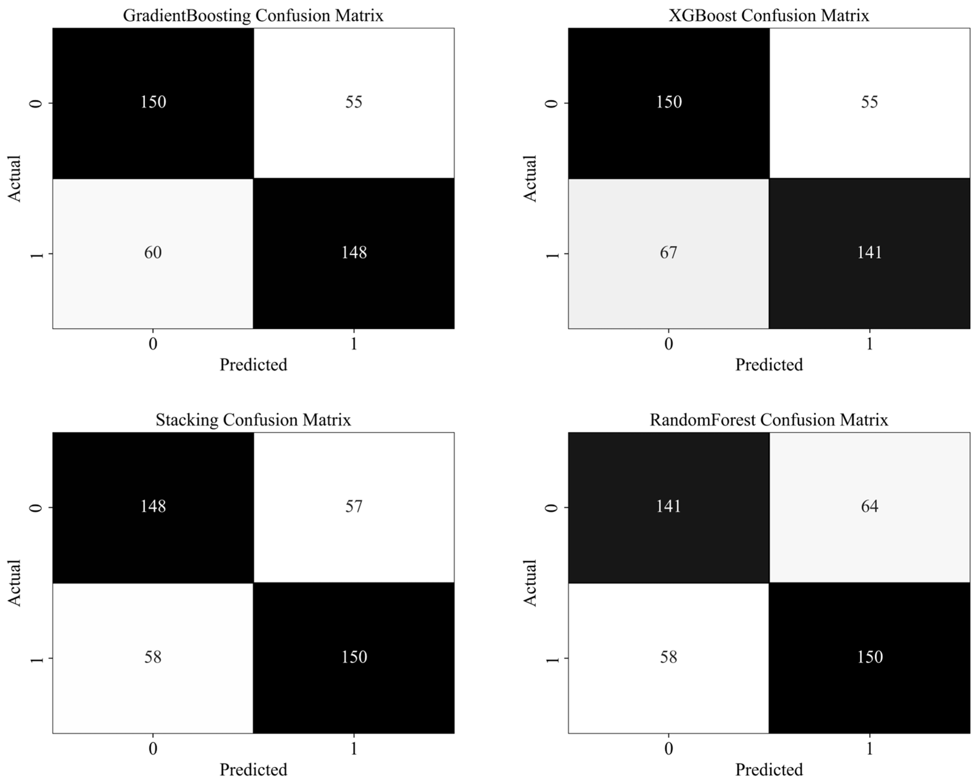
A confusion matrix provides a comprehensive, quantitative assessment of a classification model’s performance. It is one of the most widely used approaches for evaluating and comparing the predictive performance of different landslide susceptibility models. In the confusion matrix approach, classification results of a landslide susceptibility model are summarized using the following parameters: (a) true positives (TPs), which is the number of positive cases (landslides points) which are correctly predicted as positive by the model; (b) true negatives (TNs), which is the number of non-landslides cases which are correctly predicted as negative by the model; (c) false positives (FPs), which is the number of negative samples (non-landslide points) which are predicted as positive by the model; and (d) false negatives (FNs), which is the number of positive points that are predicted as negative by the model. From the confusion matrix, the following indices, which are usually used for evaluation of models, are derived: sensitivity, specificity, precision, accuracy and F-score [109,112,113].

Sensitivity, which is also called recall, expresses the proportion of positive cases correctly predicted [114]; this is often thought of as the primary statistic used to convey a model’s capacity for prediction. Conversely, specificity is the percentage of negative cases that are accurately predicted [114]. Precision describes the reliability or correctness of the model’s predictions. Accuracy is the proportion of cases correctly classified across the entire dataset, whether positive or negative. Lastly, but not least, F-score, also called F1-score, is a composite indicator of model performance that is calculated as the harmonic mean of precision and sensitivity [115]. These additional confusion-matrix-derived threshold-specific model performance evaluation parameters provide a robust way to evaluate landslide susceptibility model results, which is often more intuitive for decision-makers than the abstract shape of an ROC curve [114].

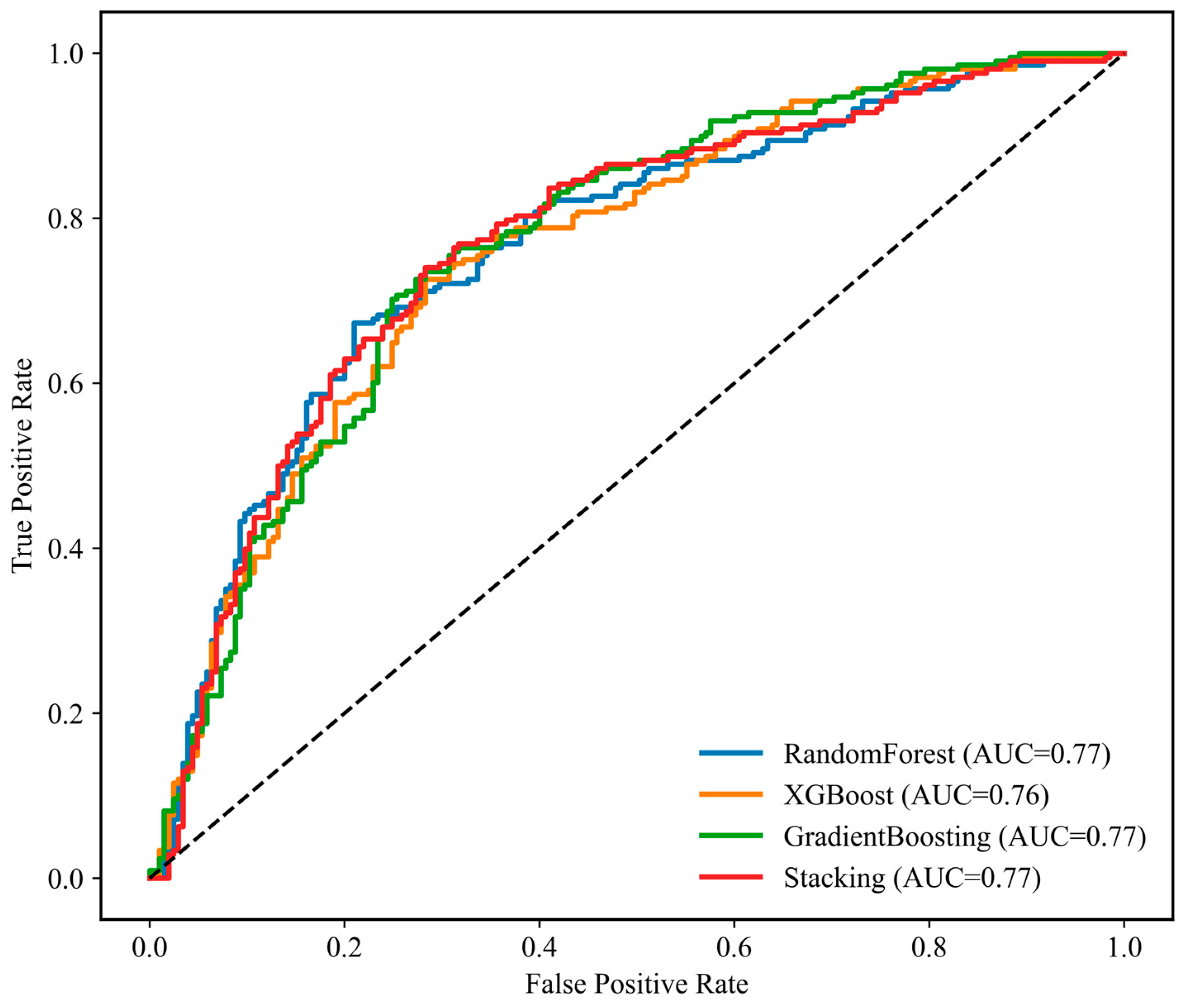
The second method that was used to evaluate susceptibility results was the ROC curve, which is a cut-off independent performance estimator [116]. It involves inspecting false positives and false negatives. A ROC curve is constructed by plotting the true positive rate (sensitivity) against the false positive rate (1 − specificity) across all possible cut-off values for each model [116]. The area under the curve (AUC) of the ROC curve quantifies the model’s overall predictive performance, representing a model’s ability to discriminate between landslide and non-landslide locations. As a quantitative indicator, the AUC reflects the goodness-of-fit and accuracy of the landslide susceptibility model [116]. A model with an AUC of 1 or close to 1 has the best performance, while an AUC of 0.5 indicates very poor performance. A landslide susceptibility map is deemed important if the AUC values approach unity, whereas a map with a value of 0.5 or lower is regarded as insignificant, as it is likely generated by chance [110]. Comparing the AUCs of ROC curves for several landslide susceptibility models allows for the evaluation of their relative efficacy in differentiating between landslide and non-landslide sites within a study area [110].

3. Results

3.1. Correlation of Landslide Conditioning Factors

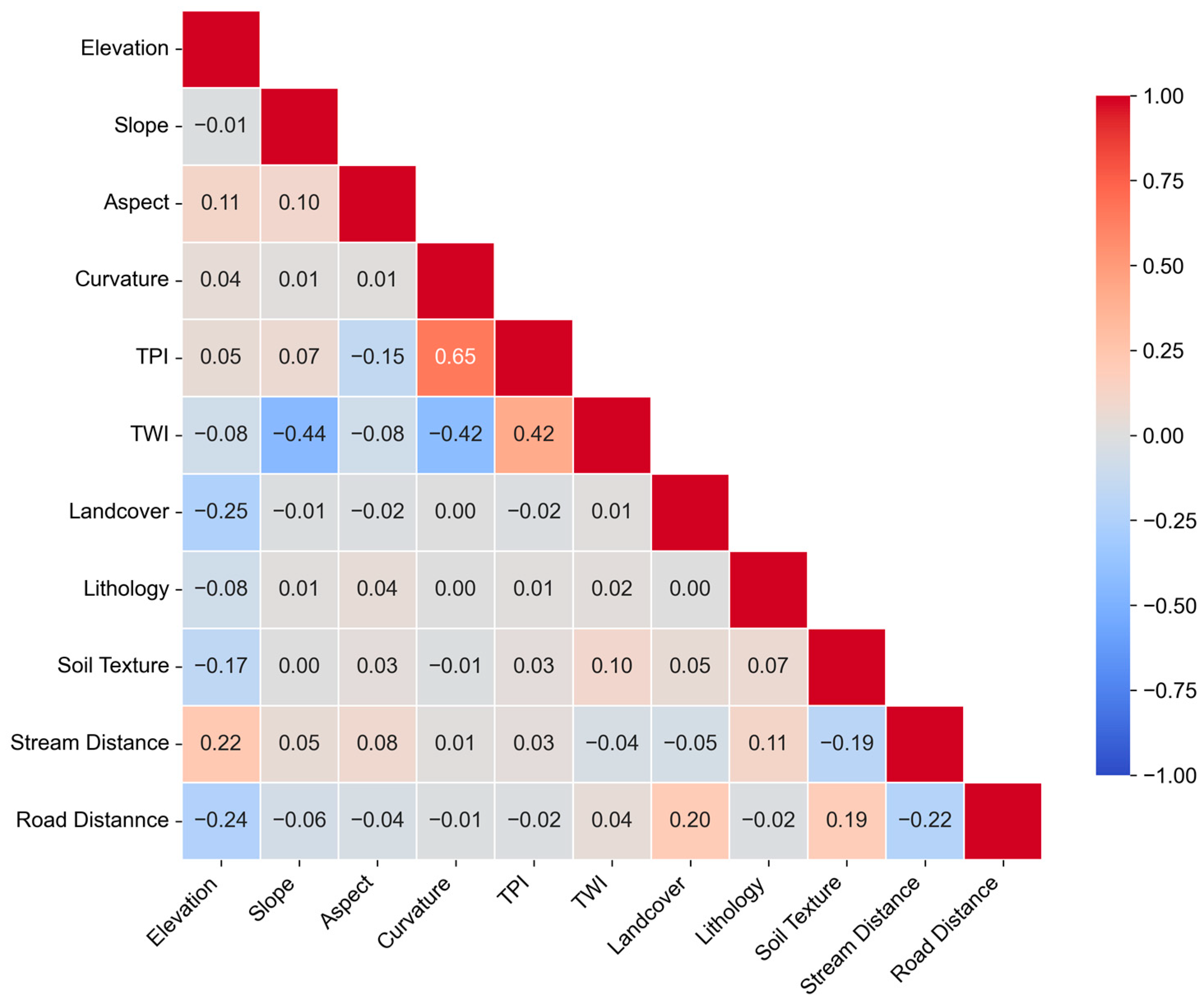
The linear correlation between the selected conditioning factors was calculated with Pearson correlation analysis. The correlation coefficients among all eleven landslide conditioning factors considered are depicted in Figure 4. The results indicate that there are no pairs of factors with a high correlation among the variables. All the factors have negligible correlations, except for a moderate correlation between TPI and curvature (0.65). Consequently, all the aforementioned landslide influencing factors were used for the landslide susceptibility assessment.

3.2. Significance of Landslide Conditioning Factors

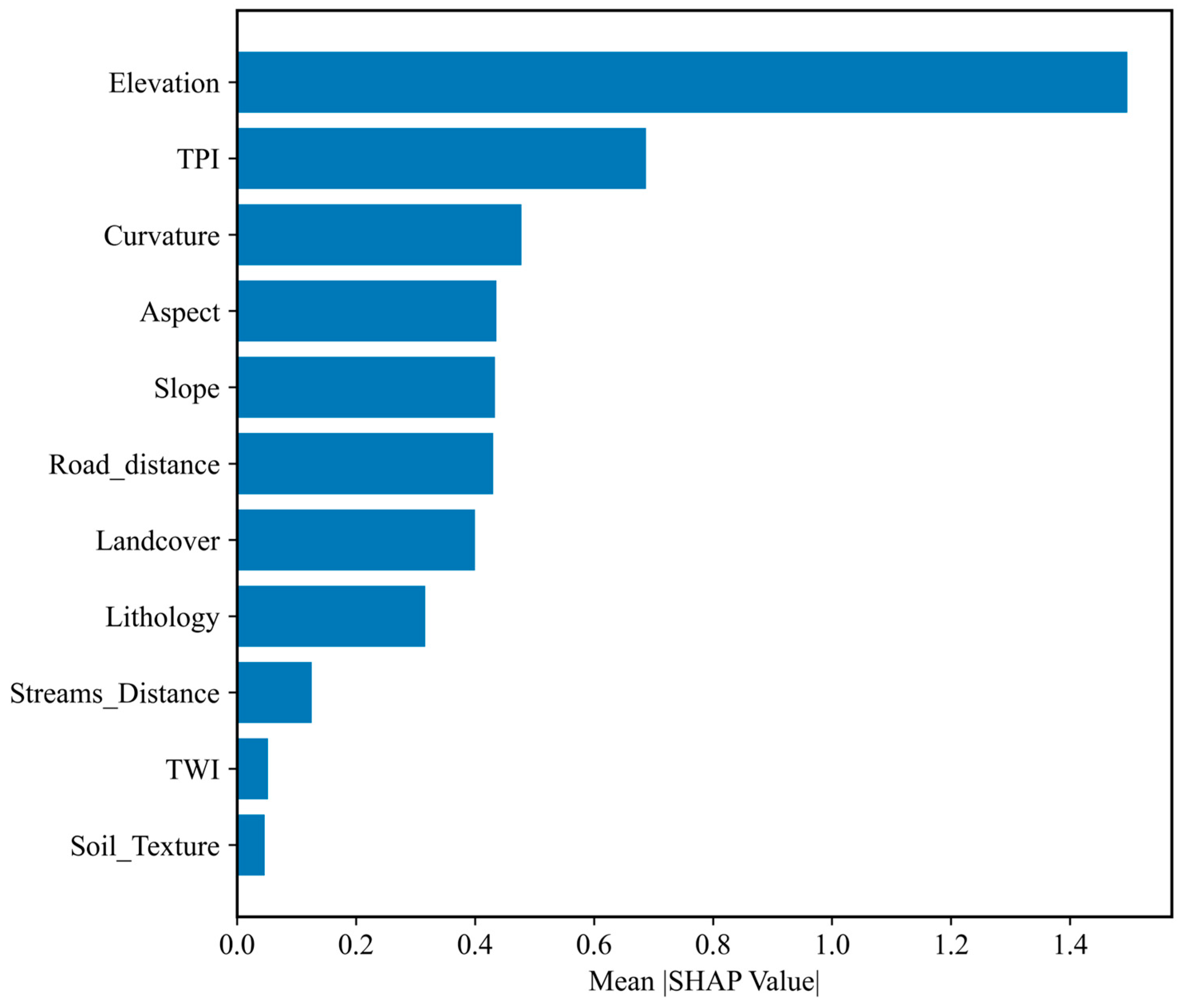
Feature importance was quantified using SHAP (SHapley Additive exPlanations) [117]. The SHAP values were computed for each feature within each model and subsequently averaged across the four machine learning algorithms to get a model-independent assessment of variable importance. Higher significance values for a conditioning factor indicate a greater influence on landslides. Such information can be useful for hazard mitigation activities, as it provides information about the landslide conditioning factors to target to reduce the potential for landslide occurrence in a specific area. For example, if the slope is highly significant, engineering measures such as terracing may be considered. The results shown in Figure 5 indicate that the most important factors for predicting landslide occurrence in the study area are elevation, TPI, curvature and slope, as they have relatively higher values, while factors such as soil texture and TWI have the lowest values. Figure 5, also shows that the SHAP values for all landslide conditioning factors are greater than zero, suggesting that the susceptibility to landslides in the studied area is influenced by each of the landslide conditioning factors included in this investigation.

3.3. Landslide Susceptibility

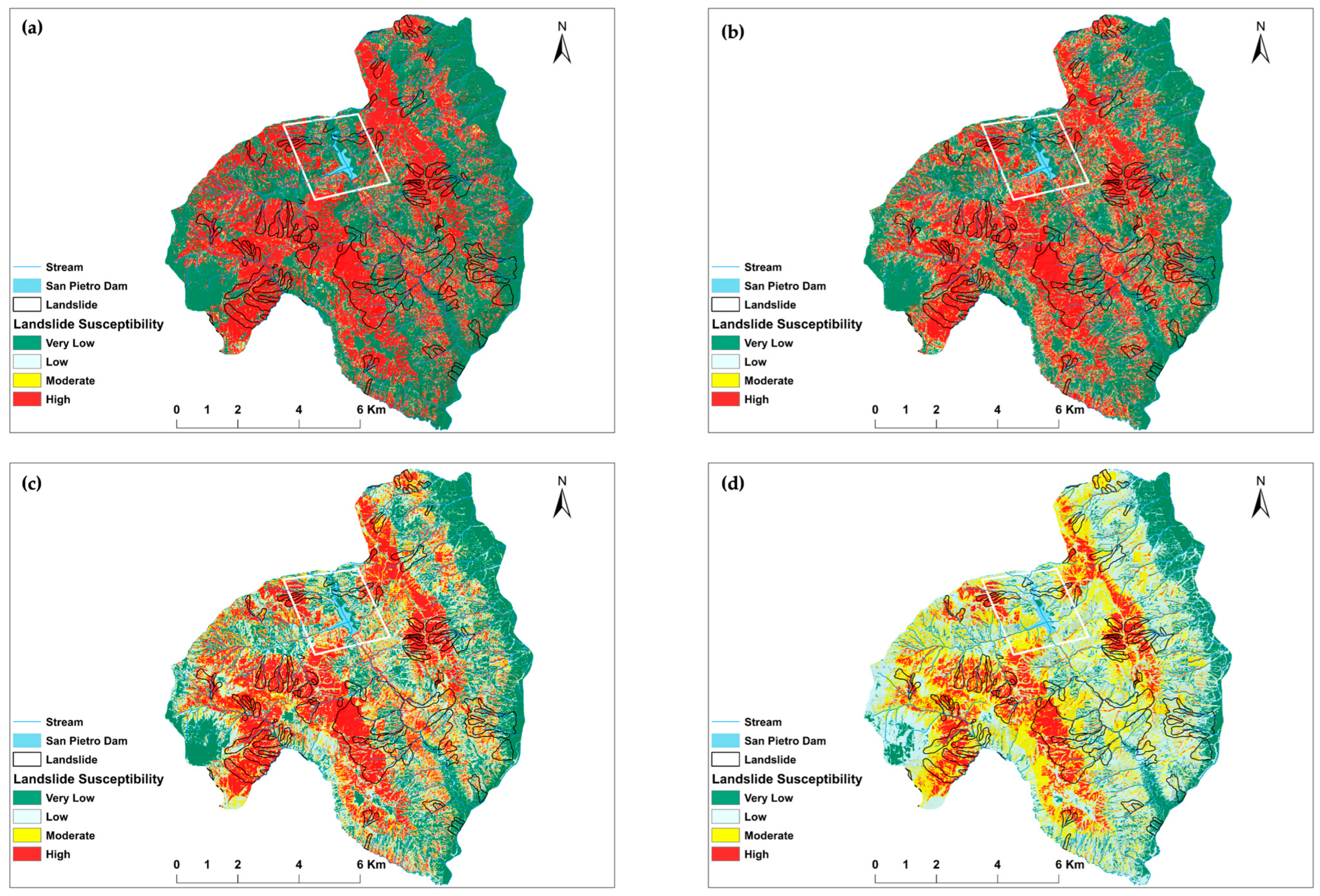
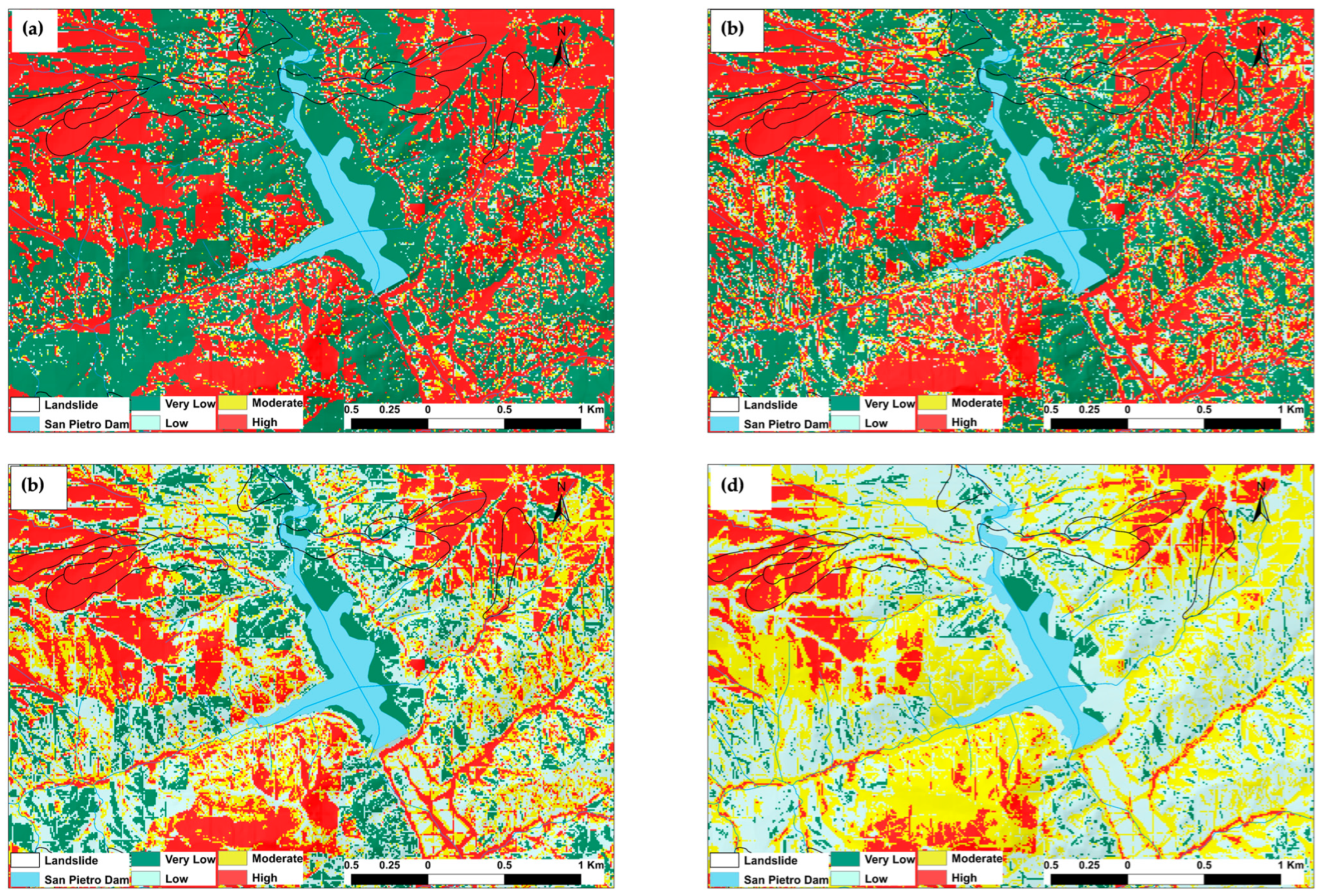
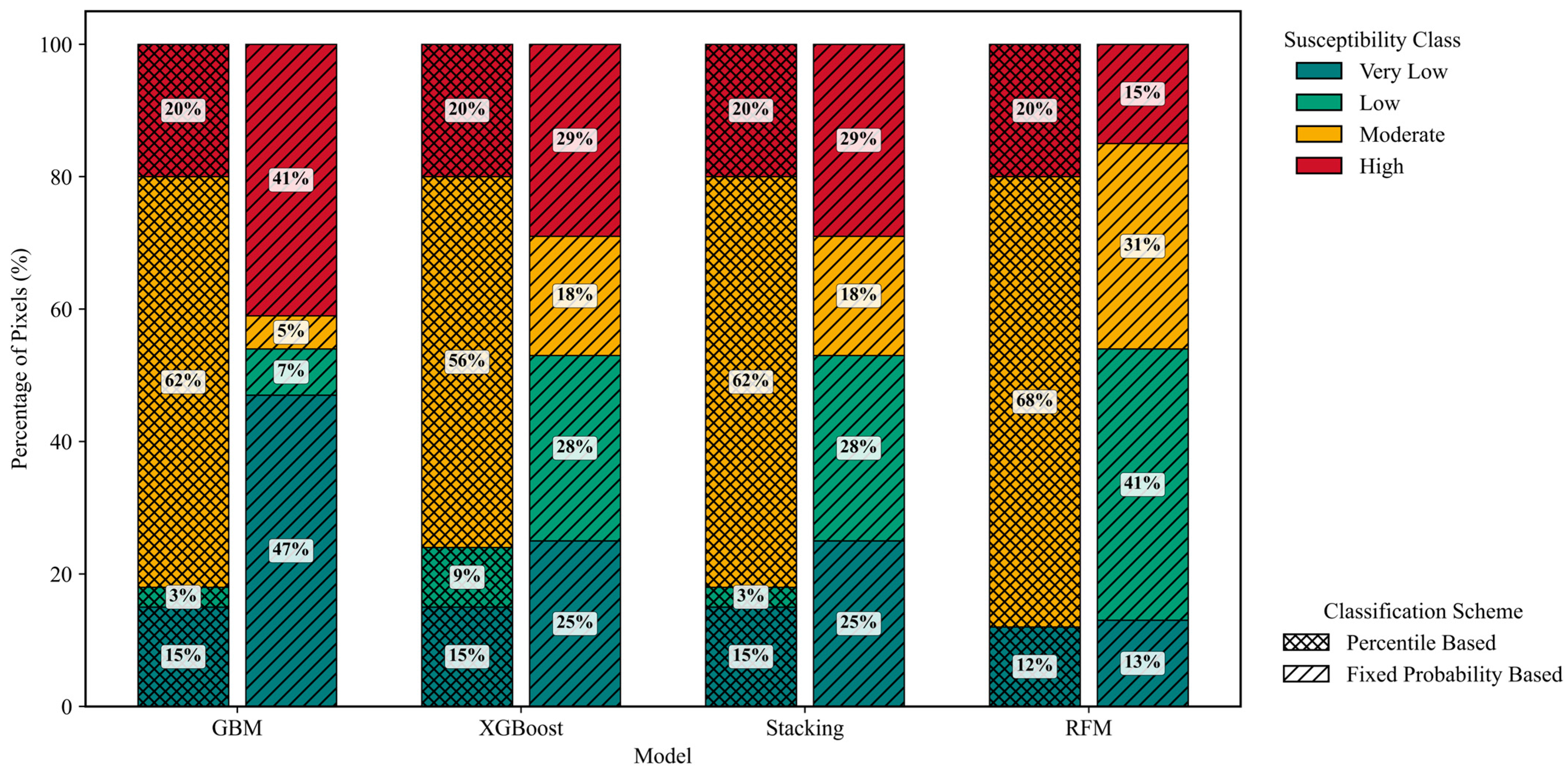
Gradient boosting machine (GBM), extreme gradient boosting (XGBoost), random forest (RF), and ensemble stacking models were used to generate landslide susceptibility maps for the study area (Figure 6 and Figure 7). The resulting landslide susceptibility maps were classified using two classification schemes. The percentile-based approach was first applied to each model separately. Thresholds for the susceptibility were defined by the 15th, 40th, and 80th percentiles of predicted landslide probabilities. This was preferred to ensure a consistent spatial ranking of susceptibility, thereby enabling objective comparison across different models. However, due to differences in probability dispersion, where predicted values cluster within a narrow range and do not exceed all percentiles across models, there was a missing class in the RF model. Because of the issue of missing classes when percentile-based classification was applied, the susceptibility maps were also classified using a fixed-probability classification scheme to allow comparison of the four models at identical risk thresholds, which is useful for operational evaluation of how the models zone the study area into different susceptibility classes. The fixed probability classes were as follows: very low (0–0.25), low (0.25–0.5), moderate (0.5–0.7), and high (0.7–1). The distribution of the percentage of pixels under different susceptibility classes for two different classification schemes is shown in Figure 8.

The analysis of the resulting susceptibility maps indicates that most parts of the landslide polygons in the landslide inventory fall within high-susceptibility classes for all four models used in this study (Figure 6). However, the distribution of susceptibility classes varies noticeably throughout the models that are employed in this study. (Figure 8). Using the presented distribution of susceptibility classes, the GBM results indicate that, when the percentile-based classification scheme is utilised, the moderate class is dominant (62%), followed by the high class (20%), then the very low class (15%), and the low class (3%). fixed-probability classification noticeably increases the high-susceptibility class (41%) and reduces the moderate class (5%), indicating overprediction. When the percentile-based scheme is used, the XGBoost model exhibits a dominant moderate class (56%), followed by the high, very low, and low classes, with 20%, 15%, and 9%, respectively. Thus, with this classification, in which a high percentage of pixels fall into the moderate class, the implication is that the model did not strongly separate stable from unstable areas. On the other hand, when fixed-probability classification is used, there is an increase in the high susceptibility class (29%) while the moderate class is reduced, indicating a shift toward higher absolute hazard estimates.

The ensemble model classifies most of the area as moderately susceptible (62%), with 20% classified as high and 15% and 3% of the pixels as very low and low, respectively. In contrast, fixed-probability thresholds increase the high-susceptibility area to 29%, with the moderate, low, and very low classes at 18%, 25%, and 28%, respectively. Thus, using fixed probabilities widely distributes the pixels into the different susceptibility classes. Lastly, under the percentile-based scheme, the RF classifies approximately 68% of the pixels as moderately susceptible, with 20% and 12% as high and very low, respectively, while the low class is missing. On the other hand, fixed-probability classification redistributes pixels toward lower susceptibility classes (very low = 13% and low = 41%) and reduces the high class (15%), with 31% of the pixels classified as moderate, indicating more conservative absolute probability estimates.

Overall, these results indicate that the percentile-based classification yields comparable susceptibility patterns across all models, with stable proportions of moderate and high hazard classes that reflect relative spatial ranking. In contrast, fixed-probability classification yields substantial model-dependent variability in hazard-class proportions, particularly for the high-susceptibility class, highlighting differences in probability scaling across algorithms. Thus, these results suggest that a percentile-based classification scheme offers a more reliable approach for inter-model comparison.

Concerning the areas immediately around the dam (Figure 7), all the used models classify as highly susceptible source areas of the landslides that have been mapped close to the reservoir. Thus, these results can be used to identify slopes that require more detailed analysis using quantitative methods, such as limit equilibrium and numerical methods.

3.4. Model Performance Assessment

As portrayed in Figure 9, the results of the AUC of the ROC curve suggest that all four landslide susceptibility models have good and comparable predictive performance. RF, GBM and Stacking models achieve the highest AUC values (AUC ≈ 0.77), while the XGBoost model follows very closely with an AUC of approximately 0.76. Among them, the ensemble-based approaches (Random Forest, Gradient Boosting, and especially the Stacking model) show slightly more stable, consistently higher true positive rates across a wide range of false positive rates, suggesting better generalisation. Overall, the models’ performances as shown by values of the AUC are higher than 0.75, which is regarded as a suitable AUC value for studies concerning landslide susceptibility assessment [14,116]. Thus, these results indicate that all four models are appropriate for mapping landslide susceptibility, with only marginal differences in performance, and that ensemble learning yields only a small advantage in predictive accuracy.

It is worthwhile noting that the validation process using the AUC of the ROC curve has some limitations, so it is not recommended to rely entirely on the corresponding results. This is because the AUC of the ROC curve is not dependent on any threshold; this means it does not assess the performance of a landslide susceptibility model using exactly the same probability thresholds that were used to classify the susceptibility map into various susceptibility categories [116]. Hence, a model may exhibit a high AUC while performing poorly when producing a classified susceptibility map [15,116]. Furthermore, the ROC curve does not provide a cost-sensitive assessment of the performance of a model, which is essential for hazard risk management decision-making [112].

To further evaluate the modelling results and enable model comparison, a confusion matrix approach was adopted, from which confusion matrix-based sensitivity, specificity, precision, accuracy, and F1-score for each model were calculated on the testing dataset and then used to evaluate the four models. These confusion-matrix-based evaluation metrics provide complementary information on model performance in landslide susceptibility classification. The confusion matrices for the four models are shown in Figure 10, with the corresponding threshold-dependent model performance metrics shown in

Table 1. Confusion matrix-based evaluation metrics for the four models.

	GBM	XGBoost	RF	Ensemble
Sensitivity	0.71	0.67	0.72	0.72
Specificity	0.73	0.73	0.69	0.72
Precision	0.73	0.72	0.70	0.72
Accuracy	0.73	0.72	0.70	0.72
F1-Score	0.72	0.70	0.71	0.72

.

Results of the confusion matrix-based performance metrics indicate that there is generally similar predictive performance, with minor variations across metrics (Table 1). In terms of sensitivity, the RF and the Ensemble model achieved the highest value (0.72), followed closely by GBM (0.71), while XGBoost recorded the lowest (0.67). For specificity, GBM and XGBoost both achieved the highest score (0.73), outperforming Random Forest (0.69), while the Ensemble model showed balanced performance (0.72). Precision values were highest for GBM (0.73), followed by XGBoost (0.72), the Ensemble model (0.72), and Random Forest (0.70). Accuracy ranged narrowly between 0.70 and 0.72, with GBM and the Ensemble model performing slightly better overall. Similarly, the F1-score values were closely clustered, with GBM and the Ensemble model achieving the highest scores (0.72), indicating a good balance between precision and recall. Overall, while all four models demonstrate comparable and satisfactory performance, GBM and the Ensemble model slightly depict superior and more consistent results across most evaluation metrics, suggesting greater robustness for landslide susceptibility prediction.

These confusion matrix-based model performance metrics provide further details on a model’s predictive capabilities and inform decision makers in selecting an appropriate model based on what they want to achieve. Generally, the four models show moderate predictive capability, but their strengths vary by metric. Furthermore, these confusion matrix-based evaluation metrics outcomes emphasize how crucial it is to evaluate the performance of landslide susceptibility models using more than just ROC-AUC evaluation results, especially when the results are to be used for the purpose of decision-making. Effective landslide susceptibility assessment requires models that show both high predictive accuracy and practical reliability in distinguishing between highly susceptible and low susceptibility zones within a study area. Overall, in this case study, the relatively high performance of the GBM and ensemble stacking models on various evaluation parameters demonstrates their appropriateness as the most efficient tools for landslide risk management in the study area.

4. Discussion

Comprehensive landslide susceptibility assessment in reservoir basins is essential for landslide risk management. Machine learning approaches are well-suited for this purpose, as they have proven to be effective across diverse environmental settings. The purpose of this study was to assess landslide susceptibility in the overall basin surrounding the San Pietro Dam, as an exploratory analysis to inform reservoir basin authorities on critical areas that may require further investigation for slope-failure hazard mitigation, with the aim of ensuring continued safe operations of the water reservoir. Such an approach to landslide susceptibility assessment at the catchment scale is considered to be innovative, since so far landslide susceptibility analysis and mitigation work have mainly focused on single slopes surrounding the dam.

Due to the scarcity of data, the analysis was performed without considering other landslide conditioning factors, such as distance to faults, soil moisture, antecedent rainfall and cumulative rainfall. Although including precipitation-related conditioning factors increases the predictive capability of landslide susceptibility models. Rainfall was not included as a conditioning factor because the study area has only one rainfall station, which made it difficult to capture the spatial variability of rainfall patterns that could inform the predictive models. Despite this limitation, the study has yielded useful results that can inform landslide risk management in the reservoir basin. Moreover, the limited number of landslide samples may have constrained machine learning models’ ability to fully capture interactions among landslide conditioning factors in the basin, which is situated in a complex geological setting. Although GBM and Ensemble models demonstrated relatively high predictive accuracy, their flexibility increases susceptibility to overfitting when training data are sparse.

The four machine learning models used in this study gave ROC AUC between 0.76 and 0.77. Additionally, the results of five statistical metrics, sensitivity, specificity, precision, accuracy, and F-1 score, indicated that all models yielded good and acceptable results, considering the scarcity of data in the study area. According to the obtained results, the ensemble stacking model did not achieve higher performance than the individual models, as expected. This outcome was not investigated extensively but may be attributable to the limited training sample size and the conditions under which this study was performed. Additionally, the GBM and RF models, whose performance was at par with the ensemble stacking model, are inherently ensembles [118]. Therefore, the variance-reduction mechanism inherent in these models may have yielded more stable predictions, upon which the ensemble stacking model could make no further improvements.

The resulting landslide susceptibility maps reveal zones that are inherently prone to slope instability, independent of specific triggering events. Concerning slopes delimiting the reservoir and those nearby, the results could be improved if reservoir-related factors, such as reservoir water-level fluctuations and in situ slope-monitoring data, were available. Nevertheless, the identified zones represent areas where dynamic factors such as reservoir water-level fluctuations or groundwater rise are likely to have the greatest effect of destabilising the slopes. Furthermore, the susceptibility maps offer a practical decision-support tool for prioritising monitoring efforts and guiding reservoir operation strategies. Therefore, the critical zones identified represent areas where detailed geotechnical investigations could be concentrated to acquire a deeper comprehension of the landslide hazard conditions in the study area.

5. Conclusions

It has been demonstrated that ML techniques can be used to generate landslide susceptibility maps for complex terrains and geological environments, and that ML models are a powerful tool for generating landslide susceptibility maps across large areas to support regional landslide management. These models can provide valuable information to identify highly susceptible areas for prioritising the implementation of hazard reduction measures. This study successfully utilised four machine learning models (GBM, XGBoost, RF and Ensemble stacking) to generate landslide susceptibility maps in a reservoir environment, providing an overview of the unstable areas in the vicinity of the dam.

The application of the four ML techniques in this study indicated that the ensemble-based approaches (Random Forest, Gradient Boosting, and the Stacking model) were equally superior, achieving the highest ROC–AUC score of 0.77. Comparative analysis of the four landslide susceptibility models using confusion matrix-based metrics demonstrates that all models provide reliable, closely comparable predictive performance. Although differences among the models are relatively small, GBM and the Ensemble model consistently show slightly superior and more balanced results across sensitivity, specificity, precision, accuracy, and F1-score. Random Forest also performs competitively, particularly in terms of sensitivity, while XGBoost achieves strong specificity and precision but slightly lower sensitivity. Overall, the findings suggest that ensemble-based and boosting techniques are effective for landslide susceptibility assessment, with GBM and the Ensemble model offering slightly stronger overall performance and greater predictive capability.

Selecting a suitable machine learning model for examining landslide susceptibility for a particular study area remains challenging, as different models have distinct advantages and limitations. Therefore, employing alternative techniques to gain deeper insights is recommended.

This work forms part of an ongoing project exploring landslides around reservoirs. Future studies should investigate the effects of reservoir operations, which alter the mechanical properties of bank-slope soils and rocks, potentially influencing the occurrence of landslides.

References

1. Yang, D.; Wu, J.; Guo, Z.; Zeng, X.; Zhang, Q. Safety risk assessment of reservoir dam structure: An empirical study in China. Sci. Rep. 2024, 14, 20232. [Google Scholar] [CrossRef]
2. Nefeslioglu, H.A.; Gorum, T. The use of landslide hazard maps to determine mitigation priorities in a dam reservoir and its protection area. Land Use Policy 2020, 91, 104363. [Google Scholar] [CrossRef]
3. Yao, C.; Li, L.; Yao, X.; Li, R.; Ren, K.; Jiang, S.; Chen, X.; Ma, L. Study on the Identification, Failure Mode, and Spatial Distribution of Bank Collapses after the Initial Impoundment in the Head Section of Baihetan Reservoir in Jinsha River, China. Remote Sens. 2024, 16, 2253. [Google Scholar] [CrossRef]
4. Stefanelli, C.T.; Casagli, N.; Catani, F. Landslide damming hazard susceptibility maps: A new GIS-based procedure for risk management. Landslides 2020, 17, 1635–1648. [Google Scholar] [CrossRef]
5. Dai, F.C.; Lee, C.F.; Deng, J.H.; Tham, L.G. The 1786 earthquake-triggered landslide dam and subsequent dam-break flood on the Dadu River, southwestern China. Geomorphology 2005, 65, 205–221. [Google Scholar] [CrossRef]
6. Fan, X.; Dufresne, A.; Siva Subramanian, S.; Strom, A.; Hermanns, R.; Tacconi Stefanelli, C.; Hewitt, K.; Yunus, A.P.; Dunning, S.; Capra, L.; et al. The formation and impact of landslide dams—State of the art. Earth-Sci. Rev. 2020, 203, 103116. [Google Scholar] [CrossRef]
7. Paronuzzi, P.; Rigo, E.; Bolla, A. Influence of filling-drawdown cycles of the Vajont reservoir on Mt. Toc slope stability. Geomorphology 2013, 191, 75–93. [Google Scholar] [CrossRef]
8. Schuster, R.L. Interaction of Dams and Landslides: Case Studies and Mitigation; US Geological Survey: Reston, VA, USA, 2006; Volume 1723, pp. 4–22. [Google Scholar]
9. Dykes, A.P.; Bromhead, E.N. The Vaiont landslide: Re-assessment of the evidence leads to rejection of the consensus. Landslides 2018, 15, 1815–1832. [Google Scholar] [CrossRef]
10. Alcântara, E.; Baião, C.F.; Guimarães, Y.C.; Marengo, J.A.; Mantovani, J.R. Climate change-induced shifts in landslide susceptibility in São Sebastião (southeastern Brazil). Nat. Hazards Res. 2025, 5, 321–334. [Google Scholar] [CrossRef]
11. Tetteh, F.K.; Abbey, S.J.; Booth, C.A.; Nukah, P.D. Current Understanding and Uncertainties Associated with Climate Change and the Impact on Slope Stability: A Systematic literature review. Nat. Hazards Res. 2025, 1446, 2669. [Google Scholar] [CrossRef]
12. Sun, J.; Li, H.; Liu, Y. Data-driven early warning indicator for the overall stability of rock slopes: An example in hydropower engineering. Environ. Model. Softw. 2024, 175, 105994. [Google Scholar] [CrossRef]
13. Lollino, P.; Giordan, D.; Allasia, P.; Fazio, N.L.; Perrotti, M.; Cafaro, F. Assessment of post-failure evolution of a large earthflow through field monitoring and numerical modelling. Landslides 2020, 17, 2013–2026. [Google Scholar] [CrossRef]
14. Guzzetti, F.; Reichenbach, P.; Cardinali, M.; Galli, M.; Ardizzone, F. Probabilistic landslide hazard assessment at the basin scale. Geomorphology 2005, 72, 272–299. [Google Scholar] [CrossRef]
15. Corominas, J.; van Westen, C.; Frattini, P.; Cascini, L.; Malet, J.P.; Fotopoulou, S.; Catani, F.; Van Den Eeckhaut, M.; Mavrouli, O.; Agliardi, F.; et al. Recommendations for the quantitative analysis of landslide risk. Bull. Eng. Geol. Environ. 2014, 73, 209–263. [Google Scholar] [CrossRef]
16. Highland, L.M.; Bobrowsky, P. The Landslide Handbook—A Guide to Understanding Landslides; US Geological Survey: Reston, VA, USA, 2008; Volume 1325, pp. 1–147. [Google Scholar]
17. Van Westen, C.J.; Castellanos, E.; Kuriakose, S.L. Spatial data for landslide susceptibility, hazard, and vulnerability assessment: An overview. Eng. Geol. 2008, 102, 112–131. [Google Scholar] [CrossRef]
18. Reichenbach, P.; Rossi, M.; Malamud, B.D.; Mihir, M.; Guzzetti, F. A review of statistically-based landslide susceptibility models. Earth Sci. Rev. 2018, 180, 60–91. [Google Scholar] [CrossRef]
19. Shano, L.; Raghuvanshi, T.K.; Meten, M. Landslide susceptibility evaluation and hazard zonation techniques—A review. Geoenviron. Disasters 2020, 7, 18. [Google Scholar] [CrossRef]
20. Van Westen, C.J.; Rengers, N.; Soeters, R. Use of Geomorphological Information in Indirect Landslide Susceptibility Assessment. Nat. Hazards 2003, 30, 399–419. [Google Scholar] [CrossRef]
21. Barredo, J.I.; Benavides, A.; Hervás, J.; Van Westen, C.J. Comparing heuristic landslide hazard assessment techniques using GIS in the Tirajana basin, Gran Canaria Island, Spain. Int. J. Appl. Earth Obs. Geoinf. 2000, 2000, 9–23. [Google Scholar] [CrossRef]
22. Van Westen, C.J.; Soeters, R.; Sijmons, K. Digital geomorphological landslide hazard mapping of the Alpago area, Italy. Int. J. Appl. Earth Obs. Geoinf. 2000, 2, 51–60. [Google Scholar] [CrossRef]
23. Zumpano, V.; Ardizzone, F.; Bucci, F.; Cardinali, M.; Fiorucci, F.; Parise, M.; Pisano, L.; Reichenbach, P.; Santaloia, F.; Santangelo, M.; et al. The relation of spatio-temporal distribution of landslides to urban development (a case study from the Apulia region, Southern Italy). J. Maps. 2021, 17, 133–140. [Google Scholar] [CrossRef]
24. Casagli, N.; Catani, F.; Puglisi, C.; Delmonaco, G.; Ermini, L.; Margottini, C. An inventory-based approach to landslide susceptibility assessment and its application to the Virginio River Basin, Italy. Environ. Eng. Geosci. 2004, 10, 203–216. [Google Scholar] [CrossRef]
25. Van Den Eeckhaut, M.; Reichenbach, P.; Guzzetti, F.; Rossi, M.; Poesen, J. Combined landslide inventory and susceptibility assessment based on different mapping units: An example from the Flemish Ardennes, Belgium. Nat. Hazards Earth Syst. Sci. 2009, 9, 507–521. [Google Scholar] [CrossRef]
26. Chalkias, C.; Polykretis, C.; Ferentinou, M.; Karymbalis, E. Integrating expert knowledge with statistical analysis for landslide susceptibility assessment at regional scale. Geosciences 2016, 6, 14. [Google Scholar] [CrossRef]
27. Malet, J.P.; Puissant, A.; Mathieu, A.; Van Den Eeckhaut, M.; Fressard, M. Integrating Spatial Multi-criteria Evaluation and Expert Knowledge for Country-Scale Landslide Susceptibility Analysis: Application to France. In Landslide Science and Practice; Margottini, C., Canuti, P., Sassa, K., Eds.; Springer: Berlin/Heidelberg, Germany, 2013. [Google Scholar] [CrossRef]
28. Zhu, A.X.; Wang, R.; Qiao, J.; Qin, C.Z.; Chen, Y.; Liu, J.; Du, F.; Lin, Y.; Zhu, T. An expert knowledge-based approach to landslide susceptibility mapping using GIS and fuzzy logic. Geomorphology 2014, 214, 128–138. [Google Scholar] [CrossRef]
29. Daniel, M.T.; Ng, T.F.; Abdul Kadir, M.F.; Pereira, J.J. Landslide Susceptibility Modeling Using a Hybrid Bivariate Statistical and Expert Consultation Approach in Canada Hill, Sarawak, Malaysia. Front. Earth Sci. 2021, 9, 616225. [Google Scholar] [CrossRef]
30. Mersha, T.; Meten, M. GIS-based landslide susceptibility mapping and assessment using bivariate statistical methods in Simada area, northwestern Ethiopia. Geoenviron. Disasters 2020, 7, 20. [Google Scholar] [CrossRef]
31. Neuhäuser, B.; Terhorst, B. Landslide susceptibility assessment using “weights-of-evidence” applied to a study area at the Jurassic escarpment (SW-Germany). Geomorphology 2007, 86, 12–24. [Google Scholar] [CrossRef]
32. Cordoba, J.P.; Mergili, M.; Aristizábal, E. Probabilistic landslide susceptibility analysis in tropical mountainous terrain using the physically based r.slope.stability model. Nat. Hazards Earth Syst. Sci. 2020, 20, 815–829. [Google Scholar] [CrossRef]
33. Lee, S.; Talib, J.A. Probabilistic landslide susceptibility and factor effect analysis. Environ. Geol. 2005, 47, 982–990. [Google Scholar] [CrossRef]
34. Sepe, C.; Calcaterra, D.; Di Martire, D.; Ramondini, M.; Russo, G.; Vitale, E.; Pappalardo, L. Landslide Susceptibility Assessment in Pyroclastic Soils: Numerical Analysis on the Role of Capillary Barriers. Ital. J. Eng. Geol. Environ. 2021, 1, 221–228. [Google Scholar] [CrossRef]
35. Armas, I.; Gheorghe, M.; Silvas, G.C. Shallow Landslides Physically Based Susceptibility Assessment Improvement Using InSAR. Case Study: Carpathian and Subcarpathian Prahova Valley, Romania. Remote Sens. 2021, 13, 2385. [Google Scholar] [CrossRef]
36. Wang, S.; Zhang, K.; van Beek, L.P.H.; Tian, X.; Bogaard, T.A. Physically-based landslide prediction over a large region: Scaling low-resolution hydrological model results for high-resolution slope stability assessment. Environ. Model. Softw. 2020, 124, 104607. [Google Scholar] [CrossRef]
37. Ugenti, A.; Angela, F.; Lucia, D.D.; Lollino, P.; Luciano, N. Moving beyond single slope quantitative analysis: A 3D slope stability assessment at urban scale. Eng. Geol. 2025, 344, 107841. [Google Scholar] [CrossRef]
38. Cafaro, F.; Cotecchia, F.; Santaloia, F.; Vitone, C.; Lollino, P.; Mitaritonna, G. Landslide hazard assessment and judgment of reliability: A geomechanical approach. Bull. Eng. Geol. Environ. 2017, 76, 397–412. [Google Scholar] [CrossRef]
39. Merghadi, A.; Yunus, A.P.; Dou, J.; Whiteley, J.; ThaiPham, B.; Bui, D.T.; Avtar, R.; Abderrahmane, B. Machine learning methods for landslide susceptibility studies: A comparative overview of algorithm performance. Earth Sci. Rev. 2020, 207, 103225. [Google Scholar] [CrossRef]
40. Ermini, L.; Catani, F.; Casagli, N. Artificial Neural Networks applied to landslide susceptibility assessment. Geomorphology 2005, 66, 327–343. [Google Scholar] [CrossRef]
41. Guo, W.; Ye, J.; Liu, C.; Lv, Y.; Zeng, Q.; Huang, X. An approach for predicting landslide susceptibility and evaluating predisposing factors. Int. J. Appl. Earth Obs. Geoinf. 2024, 135, 104217. [Google Scholar] [CrossRef]
42. Mehrabi, M.; Moayedi, H. Landslide susceptibility mapping using artificial neural network tuned by metaheuristic algorithms. Environ. Earth Sci. 2021, 80, 804. [Google Scholar] [CrossRef]
43. Lu, M.; Tay, L.T.; Mohamad-Saleh, J. Landslide susceptibility analysis using random forest model with SMOTE-ENN resampling algorithm. Geomat. Nat. Hazards Risk 2024, 15, 2314565. [Google Scholar] [CrossRef]
44. Sun, D.; Wen, H.; Wang, D.; Xu, J. A random forest model of landslide susceptibility mapping based on hyperparameter optimization using Bayes algorithm. Geomorphology 2020, 362, 107201. [Google Scholar] [CrossRef]
45. Wang, S.; Zhuang, J.; Zheng, J.; Fan, H.; Kong, J.; Zhan, J. Application of Bayesian Hyperparameter Optimized Random Forest and XGBoost Model for Landslide Susceptibility Mapping. Front. Earth Sci. 2021, 91, 617. [Google Scholar] [CrossRef]
46. Ballabio, C.; Sterlacchini, S. Support Vector Machines for Landslide Susceptibility Mapping: The Staffora River Basin Case Study, Italy. Math. Geosci. 2012, 44, 47–70. [Google Scholar] [CrossRef]
47. Kumar, D.; Thakur, M.; Dubey, C.S.; Shukla, D.P. Landslide susceptibility mapping & prediction using Support Vector Machine for Mandakini River Basin, Garhwal Himalaya, India. Geomorphology 2017, 295, 115–125. [Google Scholar] [CrossRef]
48. Marjanović, M.; Kovačević, M.; Bajat, B.; Voženílek, V. Landslide susceptibility assessment using SVM machine learning algorithm. Eng. Geol. 2011, 123, 225–234. [Google Scholar] [CrossRef]
49. Ado, M.; Amitab, K.; Maji, A.K.; Jasińska, E.; Gono, R.; Leonowicz, Z.; Jasiński, M. Landslide Susceptibility Mapping Using Machine Learning: A Literature Survey. Remote Sens. 2022, 14, 3029. [Google Scholar] [CrossRef]
50. Ilinca, V.; Șandric, I.; Gheuca, I. Geomorphology Landslide susceptibility analysis using machine learning: Insights from the bend Subcarpathians-Carpathians, Romania. Geomorphology 2025, 486, 109872. [Google Scholar] [CrossRef]
51. He, C.; Hu, X.; Tannant, D.D.; Tan, F.; Zhang, Y.; Zhang, H. Response of a landslide to reservoir impoundment in model tests. Eng. Geol. 2018, 247, 84–93. [Google Scholar] [CrossRef]
52. Zhang, Y.; Hu, X.; Tannant, D.D.; Zhang, G.; Tan, F. Field monitoring and deformation characteristics of a landslide with piles in the Three Gorges Reservoir area. Landslides 2018, 15, 581–592. [Google Scholar] [CrossRef]
53. Jones, F.O.; Embody, D.R.; Peterson, W.L.; Hazlewood, R.M. Landslides Along the Columbia River Valley, Northeastern Washington; with a Section on Seismic Surveys in Professional Paper 367; U.S. Government Printing Office: Washington, DC, USA, 1961; pp. 6–40. [CrossRef]
54. Liu, G.; Wang, B.; Sun, Q.; Hu, J.; Liu, L.; Zheng, W.; Zou, L. New insights into the Reservoir landslide deformation mechanism from InSAR and numerical simulation technology. IEEE J. Sel. Top. Appl. Earth Obs. Remote Sens. 2025, 18, 2908–2927. [Google Scholar] [CrossRef]
55. Guo, Z.; Chen, L.; Yin, K.; Shrestha, D.P.; Zhang, L. Quantitative risk assessment of slow-moving landslides from the viewpoint of decision-making: A case study of the Three Gorges Reservoir in China. Eng. Geol. 2020, 273, 105667. [Google Scholar] [CrossRef]
56. Iqbal, J.; Tu, X.; Xu, L. Landslide Hazards in Reservoir Areas: Case Study of Xiangjiaba Reservoir, Southwest China. Nat. Hazards Rev. 2017, 18, 04017009. [Google Scholar] [CrossRef]
57. Li, Y.; Xie, X.; Jin, B.; Chen, L.; Liang, X.; Yin, K. Comprehensive risk management of reservoir landslide-tsunami hazard chains: A case study of the Liangshuijing landslide in the Three Gorges Reservoir area. Landslides 2024, 22, 671–691. [Google Scholar] [CrossRef]
58. Yin, Y.P.; Huang, B.; Chen, X.; Liu, G.; Wang, S. Numerical analysis on wave generated by the Qianjiangping landslide in Three Gorges Reservoir, China. Landslides 2015, 12, 355–364. [Google Scholar] [CrossRef]
59. Yin, Y.; Huang, B.; Wang, W.; Wei, Y.; Ma, X.; Ma, F.; Zhao, C. Reservoir-induced landslides and risk control in Three Gorges Project on Yangtze River, China. J. Rock. Mech. Geotech. Eng. 2016, 8, 577–595. [Google Scholar] [CrossRef]
60. Cusano, A.; Russo, F.; Guerriero, L.; Colucciello, A.; Ruzza, G.; Guadagno, F.M.; Revellino, P. Geotourism, traditions and typical products of Avellino Province. J. Maps. 2022, 18, 133–141. [Google Scholar] [CrossRef]
61. Sisto, M.; Di Lisio, A.; Russo, F. Geosite Assessment as a Tool for the Promotion and Conservation of Irpinia Landscape Geoheritage (Southern Italy). Resources 2022, 11, 97. [Google Scholar] [CrossRef]
62. Carminati, E.; Doglioni, C. Alps vs. Apennines: The paradigm of a tectonically asymmetric Earth. Earth-Sci. Rev. 2012, 112, 67–96. [Google Scholar] [CrossRef]
63. Vezzani, L.; Festa, A.; Ghisetti, F.C. Geology and Tectonic Evolution of the Central-Southern Apennines, Italy. Geol. Soc. Am. 2010, 469, 2–25. [Google Scholar] [CrossRef]
64. Mario, B.; Giacomo, P.; Paola, G.; Giuseppe, P.; Marco, P.; Katia, S.; Francesco, C. Landslides and predisposing factors of the Southern Apennines, Italy. J. Maps. 2023, 19, 2137065. [Google Scholar] [CrossRef]
65. Vitagliano, E.; Improta, L.; Pizzino, L.; D’Agostino, N. Study of well data reveals fluid pressure distribution and origin in the upper crust of the Irpinia region (Southern Apennines, Italy). Tectonophysics 2025, 908, 230761. [Google Scholar] [CrossRef]
66. Di Nocera, S.; Matano, F.; Pescatore, T.S.; Pinto, F.; Quarantiello, R.; Senatore, M.R.; Torre, M.L. Geological scheme of the transect Eastern Picentini-Southern Daunia Mts.: Stratigraphic units and tectonic evolution of the outer zones of the Southern Apennines, Italy. Boll. Soc. Geol. Ital. 2006, 125, 39–58. [Google Scholar]
67. Trigila, A.; Frattini, P.; Casagli, N.; Catani, F.; Crosta, G.; Esposito, C.; Iadanza, C.; Lagomarsino, D.; Mugnozza, G.S.; Segoni, S. Landslide Susceptibility Mapping at National Scale: The Italian Case Study. In Landslide Science and Practice; Margottini, C., Ed.; Springer: Berlin/Heidelberg, Germany, 2013; Volume 1, pp. 287–295. [Google Scholar] [CrossRef]
68. Guzzetti, F.; Mondini, A.C.; Cardinali, M.; Fiorucci, F.; Santangelo, M.; Chang, K.T. Landslide inventory maps: New tools for an old problem. Earth Sci. Rev. 2012, 112, 42–66. [Google Scholar] [CrossRef]
69. Galli, M.; Ardizzone, F.; Cardinali, M.; Guzzetti, F.; Reichenbach, P. Comparing landslide inventory maps. Geomorphology 2008, 94, 268–289. [Google Scholar] [CrossRef]
70. Malamud, B.D.; Turcotte, D.L.; Guzzetti, F.; Reichenbach, P. Landslide inventories and their statistical properties. Earth Surf. Process Landf. 2004, 29, 687–711. [Google Scholar] [CrossRef]
71. Fell, R.; Corominas, J.; Bonnard, C.; Cascini, L.; Leroi, E.; Savage, W.Z. Guidelines for landslide susceptibility, hazard and risk zoning for land use planning. Eng. Geol. 2008, 102, 85–98. [Google Scholar] [CrossRef]
72. Tarquini, S.; Isola, I.; Favalli, M.; Mazzarini, F.; Bisson, M.; Pareschi, M.T.; Boschi, E. TINITALY/01: A new Triangular Irregular Network of Italy. Ann. Geophys. 2009, 50, 407–425. [Google Scholar] [CrossRef]
73. Çellek, S. Effect of the slope angle and its classification on landslides. Nat. Hazards Earth Syst. Sci. 2020, 87, 85–95. [Google Scholar] [CrossRef]
74. Bathrellos, G.D.; Koukouvelas, I.K.; Skilodimou, H.D.; Nikolakopoulos, K.G.; Vgenopoulos, A.L. Landslide causative factors evaluation using GIS in the tectonically active Glafkos River area, northwestern Peloponnese, Greece. Geomorphology 2024, 461, 109285. [Google Scholar] [CrossRef]
75. Cellek, S. The Effect of Aspect on Landslide and Its Relationship with Other Parameters. In Landslides; Zhang, Y., Cheng, Q., Eds.; IntechOpen: London, UK, 2022; pp. 8–25. [Google Scholar] [CrossRef]
76. Gorokhovich, Y.; Vustianiuk, A. Implications of slope aspect for landslide risk assessment: A case study of Hurricane Maria in Puerto Rico in 2017. Geomorphology 2021, 391, 107874. [Google Scholar] [CrossRef]
77. Hidayat, S.; Pachri, H.; Alimuddin, I. Analysis of Landslide Susceptibility Zone using Frequency Ratio and Logistic Regression Method in Hambalang, Citeureup District, Bogor Regency, West Java Province. IOP Conf. Ser. Earth Environ. Sci. 2019, 280, 12005. [Google Scholar] [CrossRef]
78. Komac, M. A landslide susceptibility model using the Analytical Hierarchy Process method and multivariate statistics in perialpine Slovenia. Geomorphology 2006, 74, 17–28. [Google Scholar] [CrossRef]
79. Rabby, Y.W.; Ishtiaque, A.; Rahman, M.S. Evaluating the effects of digital elevation models in landslide susceptibility mapping in rangamati district, Bangladesh. Remote Sens. 2020, 12, 2718. [Google Scholar] [CrossRef]
80. Emberson, R.; Kirschbaum, D.B.; Amatya, P.; Tanyas, H.; Marc, O. Insights from the topographic characteristics of a large global catalog of rainfall-induced landslide event inventories. Nat. Hazards Earth Syst. Sci. 2022, 22, 1129–1149. [Google Scholar] [CrossRef]
81. Meena, S.R.; Puliero, S.; Bhuyan, K.; Floris, M.; Catani, F. Assessing the importance of conditioning factor selection in landslide susceptibility for the province of Belluno (region of Veneto, northeastern Italy). Nat. Hazards Earth Syst. Sci. 2022, 22, 1395–1417. [Google Scholar] [CrossRef]
82. Yang, D.; Qiu, H.; Hu, S.; Pei, Y.; Wang, X.; Du, C.; Long, Y.; Cao, M. Influence of successive landslides on topographic changes revealed by multitemporal high-resolution UAS-based DEM. Catena 2021, 202, 105229. [Google Scholar] [CrossRef]
83. Glade, T. Landslide Hazard Assessment and Historical Landslide Data—An Inseparable Couple? In The Use of Historical Data in Natural Hazard Assessments; Glade, T., Albini, P., Francés, F., Eds.; Springer: Dordrecht, The Netherlands, 2001; Volume 17, pp. 153–168. [Google Scholar] [CrossRef]
84. Lann, T.; Bao, H.; Lan, H.; Zheng, H.; Yan, C.; Peng, J. Hydro-mechanical effects of vegetation on slope stability: A review. Sci. Total Environ. 2024, 926, 171691. [Google Scholar] [CrossRef]
85. Zhang, J.; Qiu, H.; Tang, B.; Yang, D.; Liu, Y.; Liu, Z.; Ye, B.; Zhou, W.; Zhu, Y. Accelerating Effect of Vegetation on the Instability of Rainfall-Induced Shallow Landslides. Remote Sens. 2022, 14, 5743. [Google Scholar] [CrossRef]
86. Copernicus Land Monitoring Service. Available online: https://land.copernicus.eu/en (accessed on 30 October 2025).
87. Bielecka, E.; Jenerowicz, A. Intellectual structure of CORINE land cover research applications in Web of Science: A Europe-wide review. Remote Sens. 2019, 11, 2017. [Google Scholar] [CrossRef]
88. Yalcin, A.; Bulut, F. Landslide susceptibility mapping using GIS and digital photogrammetric techniques: A case study from Ardesen (NE-Turkey). Nat. Hazards 2007, 41, 201–226. [Google Scholar] [CrossRef]
89. Temme, A.J.A.M. Relations Between Soil Development and Landslides. In Hydrogeology, Chemical Weathering, and Soil Formation, 1st ed.; Hunt, A., Egli, M., Faybishenko, B., Eds.; John Wiley and Sons, Inc.: Hoboken, NJ, USA, 2021; pp. 177–185. [Google Scholar] [CrossRef]
90. Ohlmacher, G.C. Plan curvature and landslide probability in regions dominated by earth flows and earth slides. Eng. Geol. 2007, 91, 117–134. [Google Scholar] [CrossRef]
91. Mathew, J.; Jha, V.K.; Rawat, G.S. Landslide susceptibility zonation mapping and its validation in part of Garhwal Lesser Himalaya, India, using binary logistic regression analysis and receiver operating characteristic curve method. Landslides 2009, 6, 17–26. [Google Scholar] [CrossRef]
92. Krkač, M.; Bernat Gazibara, S.; Sinčić, M.; Lukačić, H.; Šarić, G.; Mihalić Arbanas, S. Impact of Input Data on the Quality of the Landslide Susceptibility Large-Scale Maps: A Case Study from NW Croatia. In Progress in Landslide Research and Technology; Alcántara-Ayala, I., Arbanas, Ž., Cuomo, S., Huntley, D., Konagai, K., Arbanas, S.M., Mikoš, M., Sassa, K., Sassa, S., Tang, H., et al., Eds.; Springer: Cham, Switzerland, 2023; Volume 2, pp. 135–146. [Google Scholar] [CrossRef]
93. Dormann, C.F.; Elith, J.; Bacher, S.; Buchmann, C.; Carl, G.; Carré, G.; Marquéz, J.R.G.; Gruber, B.; Lafourcade, B.; Leitão, P.J.; et al. Collinearity: A review of methods to deal with it and a simulation study evaluating their performance. Ecography 2013, 36, 27–46. [Google Scholar] [CrossRef]
94. Akgun, A.; Türk, N. Landslide susceptibility mapping for Ayvalik (Western Turkey) and its vicinity by multicriteria decision analysis. Environ. Earth Sci. 2010, 61, 595–611. [Google Scholar] [CrossRef]
95. Acharya, V.; Ghosh, A.; Kang, I.; Munasinghe, T.; Binita, K.C. Landslide Likelihood Prediction using Machine Learning Algorithms. In Proceedings of the 2022 IEEE International Conference on Big Data, Osaka, Japan, 17–20 December 2022; pp. 5395–5403. [Google Scholar] [CrossRef]
96. Ali, N.; Chen, J.; Fu, X.; Ali, R.; Hussain, M.A.; Daud, H.; Hussain, J.; Altalbe, A. Integrating Machine Learning Ensembles for Landslide Susceptibility Mapping in Northern Pakistan. Remote Sens. 2024, 16, 988. [Google Scholar] [CrossRef]
97. Zhang, A.; Zhao, X.-W.; Zhao, X.-Y.; Zheng, X.-Z.; Zeng, M.; Huang, X.; Wu, P.; Jiang, T.; Wang, S.-C.; He, J.; et al. Comparative study of different machine learning models in landslide susceptibility assessment: A case study of Conghua District, Guangzhou, China. China Geol. 2024, 7, 104–115. [Google Scholar] [CrossRef]
98. Breiman, L. Random Forests. Mach. Learn. 2001, 45, 5–32. [Google Scholar] [CrossRef]
99. Hussain, M.A.; Chen, Z.; Zheng, Y.; Shoaib, M.; Shah, S.U.; Ali, N.; Afzal, Z. Algorithm Validated by Persistent Scatterer In-SAR Technique. Sensors 2022, 22, 3119. [Google Scholar] [CrossRef]
100. Friedman, J.H. Greedy Function Approximation: A Gradient Boosting Machine. Ann. Stat. 2001, 29, 1189–1232. [Google Scholar] [CrossRef]
101. Natekin, A.; Knoll, A. Gradient boosting machines, a tutorial. Front. Neurorobot. 2013, 7, 21. [Google Scholar] [CrossRef] [PubMed]
102. Soodabeh, A.; Manfred, V. A Learning Rate Method for Full-Batch Gradient Descent. Műszaki Tudományos Közlemények 2020, 13, 174–177. [Google Scholar] [CrossRef]
103. Ravaut, M.; Gorti, S. Gradient descent revisited via an adaptive online learning rate. arXiv 2018. [Google Scholar] [CrossRef]
104. Zhang, W.; He, Y.; Wang, L.; Liu, S.; Meng, X. Landslide Susceptibility mapping using random forest and extreme gradient boosting: A case study of Fengjie, Chongqing. Geol. J. 2023, 58, 2372–2387. [Google Scholar] [CrossRef]
105. Di Napoli, M.; Carotenuto, F.; Cevasco, A.; Confuorto, P.; Di Martire, D.; Firpo, M.; Pepe, G.; Raso, E.; Calcaterra, D. Machine learning ensemble modelling as a tool to improve landslide susceptibility mapping reliability. Landslides 2020, 17, 1897–1914. [Google Scholar] [CrossRef]
106. Puspita, T. Bayesian Hyperparameter Optimization Analysis for Sustainable Innovation Performance Prediction Model. Eig. Math. J. 2025, 8, 147–162. [Google Scholar] [CrossRef]
107. Frattini, P.; Crosta, G.; Carrara, A. Techniques for evaluating the performance of landslide susceptibility models. Eng. Geol. 2010, 111, 62–72. [Google Scholar] [CrossRef]
108. Fleuchaus, P.; Blum, P.; Wilde, M.; Terhorst, B.; Butscher, C. Retrospective evaluation of landslide susceptibility maps and review of validation practice. Environ. Earth Sci. 2021, 80, 485. [Google Scholar] [CrossRef]
109. Parra, F.; González, J.; Chacón, M.; Marín, M. Modeling and Evaluation of the Susceptibility to Landslide Events Using Machine Learning Algorithms in the Province of Chañaral, Atacama Region, Chile. Nat. Hazards Earth Syst. Sci. Discuss. 2023, 15, 16806. [Google Scholar] [CrossRef]
110. Lagomarsino, D.; Tofani, V.; Segoni, S.; Catani, F.; Casagli, N. A Tool for Classification and Regression Using Random Forest Methodology: Applications to Landslide Susceptibility Mapping and Soil Thickness Modeling. Environ. Model. Assess. 2017, 22, 201–214. [Google Scholar] [CrossRef]
111. Song, Y.; Yang, D.; Wu, W.; Zhang, X.; Zhou, J.; Tian, Z.; Wang, C.; Song, Y. Evaluating Landslide Susceptibility Using Sampling Methodology and Multiple Machine Learning Models. ISPRS Int. J. Geo-Inform. 2023, 12, 197. [Google Scholar] [CrossRef]
112. Xu, Q.; Yordanov, V.; Amici, L.; Brovelli, M.A. Landslide susceptibility mapping using ensemble machine learning methods: A case study in Lombardy, Northern Italy. Int. J. Digit. Earth 2024, 17, 2346263. [Google Scholar] [CrossRef]
113. Begueria, S. Validation and Evaluation of Predictive Models in Hazard Assessment and Risk Management. Nat. Hazards 2006, 37, 315–329. [Google Scholar] [CrossRef]
114. Yu, L.; Pradhan, B.; Wang, Y. A comparative study of various combination strategies for landslide susceptibility mapping considering landslide types. Geosci. Front. 2024, 16, 101999. [Google Scholar] [CrossRef]
115. Calì, C.; Longobardi, M. Some mathematical properties of the ROC curve and their applications. Ric. Mat. 2015, 64, 391–402. [Google Scholar] [CrossRef]
116. Baddeley, A.; Rubak, E.; Rakshit, S.; Nair, G. ROC curves for spatial point patterns and presence-absence data. arXiv 2025. [Google Scholar] [CrossRef]
117. Lundberg, S.M.; Lee, S.; Lundberg, S.M.; Lee, S.I. A unified approach to interpreting model predictions. In NIPS’17: Proceedings of the 31st International Conference on Neural Information Processing Systems, Long Beach, CA, USA, 4–9 December 2017; Curran Associates Inc.: Red Hook, NY, USA, 2017; Volume 32, pp. 4765–4774. [Google Scholar]
118. Sahin, E.K. Assessing the predictive capability of ensemble tree methods for landslide susceptibility mapping using XGBoost, gradient boosting machine, and random forest. SN Appl. Sci. 2020, 2, 1308. [Google Scholar] [CrossRef]
Figure 1. Map of the study area. Insert: location of the study area in Southern Italy (boundary between Aquilonia and Montverde towns) indicated by a red dot.
Geosciences 16 00153 g001
Figure 2. Landslide inventory map for the study area, with landslides classified by type.
Geosciences 16 00153 g002
Figure 3. Relationship between landslide frequency density (f) and landslide area (A), both on logarithmic axes.
Geosciences 16 00153 g003
Figure 4. Pearson correlation coefficient matrix for different landslide conditioning factors used in this study.
Geosciences 16 00153 g004
Figure 5. Significance of landslide conditioning factors used in the study based on the average SHAP values of all four ML models.
Geosciences 16 00153 g005
Figure 6. Landslide susceptibility maps derived from different machine learning techniques: (a) GBM model, (b) XGBoost model, (c) Ensemble stacking model and (d) RF model. The area close to the dam, demarcated by a white rectangle, is zoomed in Figure 7.
Geosciences 16 00153 g006
Figure 7. Zoom in on the area closest to the dam showing landslide susceptibility distribution: (a) GBM model, (b) XGBoost model, (c) Ensemble stacking model and (d) RF model.
Geosciences 16 00153 g007
Figure 8. Percentage of pixels under different susceptibility classes for the landslide susceptibility model used in this study.
Geosciences 16 00153 g008
Figure 9. ROC curves for the different ML models.
Geosciences 16 00153 g009
Figure 10. Confusion matrices for the four landslide susceptibility models used in this study.
Geosciences 16 00153 g010