


Abstract
This study evaluates the performance of eleven Planetary Boundary Layer (PBL) schemes within the Weather Research and Forecasting (WRF) model over the Central Amazon Basin, focusing on contrasting wet and dry season conditions observed during the GoAmazon2014/5 campaign. High-resolution (1 km) simulations were conducted for representative periods in each season and validated against in situ observations. Model performance was assessed using multiple statistical metrics with the explicit separation of daytime convective and nighttime stable PBL regimes. Results reveal substantial variability among PBL schemes, strongly modulated by the season and diurnal cycle. Overall performance was higher during the wet period, whereas dry period simulations exhibited larger uncertainties, particularly under nocturnal conditions. The Shin–Hong (SH) PBL scheme had the best skill on average to reproduce the observed PBL height (PBLH) during the wet period, while the University of Washington (UW) PBL scheme was the best during the dry period. The Mellor–Yamada–Janjic (MYJ) PBL scheme had the best skill for daytime PBLH in both periods. Spatial analysis demonstrated how PBL schemes impact the PBLH distribution over the Central Amazon Basin, revealing a river-influenced pattern. These findings highlight the strong sensitivity of the Amazon PBL depth to PBL schemes and underscore the importance of appropriate PBL parameterizations and the vertical resolution for tropical applications.
1. Introduction
Numerical Weather Prediction (NWP) models are unable to fully resolve the physical subgrid-scale processes due to constraints associated with the numerical resolution, for instance, the feasibility of computing resources and their expensive costs to solve the complete physics particularly for operational ends [1]. Therefore, different parameterization schemes handle these subgrid-scale physical processes during the model run and are a component of primary importance [2,3]. Vertical turbulent mixing is a source of uncertainty in NWP models and is parameterized assuming that the Planetary Boundary Layer (PBL) is horizontally homogeneous [4].
A PBL parameterization scheme determines vertical profiles of subgrid-scale fluxes in terms of resolved variables, either diagnosing the vertical turbulent mixing or predicting it by employing different turbulence closure models, a mixing treatment, and PBL height (PBLH) estimation methods [5,6]. The physical representation and formulation of PBL schemes have advanced over the last decades covering different stability regimes and PBL features, such as non-local transport and entrainment processes [7,8,9,10,11,12,13,14,15,16,17]. PBL schemes are often classified based on the turbulence closure order and mixing treatment: local PBL schemes are developed to work under stable stratification conditions due to their small-eddies local mixing, while non-local PBL schemes focus on unstable stratification due to their ability to account for large-eddy effects [6]. Several studies reported the impacts of PBL schemes and importance of the accurate prediction of PBL parameters on NWP, climate modeling, pollutant dispersion simulations, and air quality prediction [18,19,20,21,22,23,24,25,26].
Many PBL schemes were tested within the Weather Research and Forecasting (WRF) model [27] under a wide range of model versions, meteorological conditions, atmospheric processes, and methodologies [21,23,24,28,29,30,31,32,33,34,35,36,37,38,39,40,41,42,43]. The fact that the suitability and performance of PBL schemes are intrinsically related to a particular characteristic, such as weather conditions, geographical features, and model configurations, generates a wide range of applicability [21]. Most of these studies focused on inferring the impact of PBL schemes over Northern Hemisphere regions by evaluating their ability to reproduce surface and PBL conditions [22]. Although some of them studied the Amazon region [39,44,45,46], some questions remain open, especially based on their performance under the pronounced different seasons (i.e., wet, dry, transition) present in the tropics.
Recent studies have tested PBL schemes to reproduce the atmospheric conditions over the Amazon Basin. Wang et al. [44] showed that simulations within the WRF model with the Yonsei University (YSU) PBL scheme could roughly capture the observed daily cycles of surface variables and turbulent heat fluxes, while the PBLH is underestimated especially at night. Wang et al. [45] tested six PBL schemes within the WRF model, such as Asymmetric Convective Model 2 (ACM2), Grenier-Bretherton-McCaa (GBM), University of Washington (UW), Mellor–Yamada–Nakanishi–Niino Level 2.5 (MYNN2.5), MYNN Level 3 (MYNN3), and YSU. Their results showed that diurnal PBLH is more accurately predicted than its underestimated nocturnal counterpart and that the UW PBL scheme performs better. Prein et al. [46] simulated Mesoscale Convective Systems (MCSs) within the WRF model by testing three PBL schemes (Mellor–Yamada–Janjic—MYJ, MYNN2.5, and YSU), for which results revealed that Amazon MCSs are more sensitive to PBL schemes than US MCSs. Mantovani Júnior et al. [39] tested eight PBL schemes for two dry periods over the Central Amazon Basin. They demonstrated that WRF predictions are sensitive to the PBL scheme selection and that the MYNN2.5 PBL scheme best reproduced the observed PBLH.
In this context, the present study focuses on the role of PBL schemes to reproduce the observed PBL over the Amazon Basin under wet and dry conditions. The study aims to assess the WRF sensitivity of the PBLH, vertical structure, and turbulent fluxes to different PBL schemes using 1-km resolution WRF simulations and in situ observations from the GoAmazon2014/5 campaign [47]. Our main scientific questions are given as follows: (i) is there a preferred PBL scheme for reproducing the observed PBLH for each period? (ii) What impact do PBL schemes have on reproducing the observed conditions at the surface and within the PBL? (iii) How does the PBL scheme impact the distribution of PBLH over the Central Amazon Basin? The paper is organized as follows: Section 2 presents the methodology and datasets; Section 3 presents the results; and Section 4 presents the discussion and final remarks.
2. Materials and Methods
2.1. Study Area and Observational Data
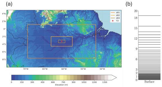
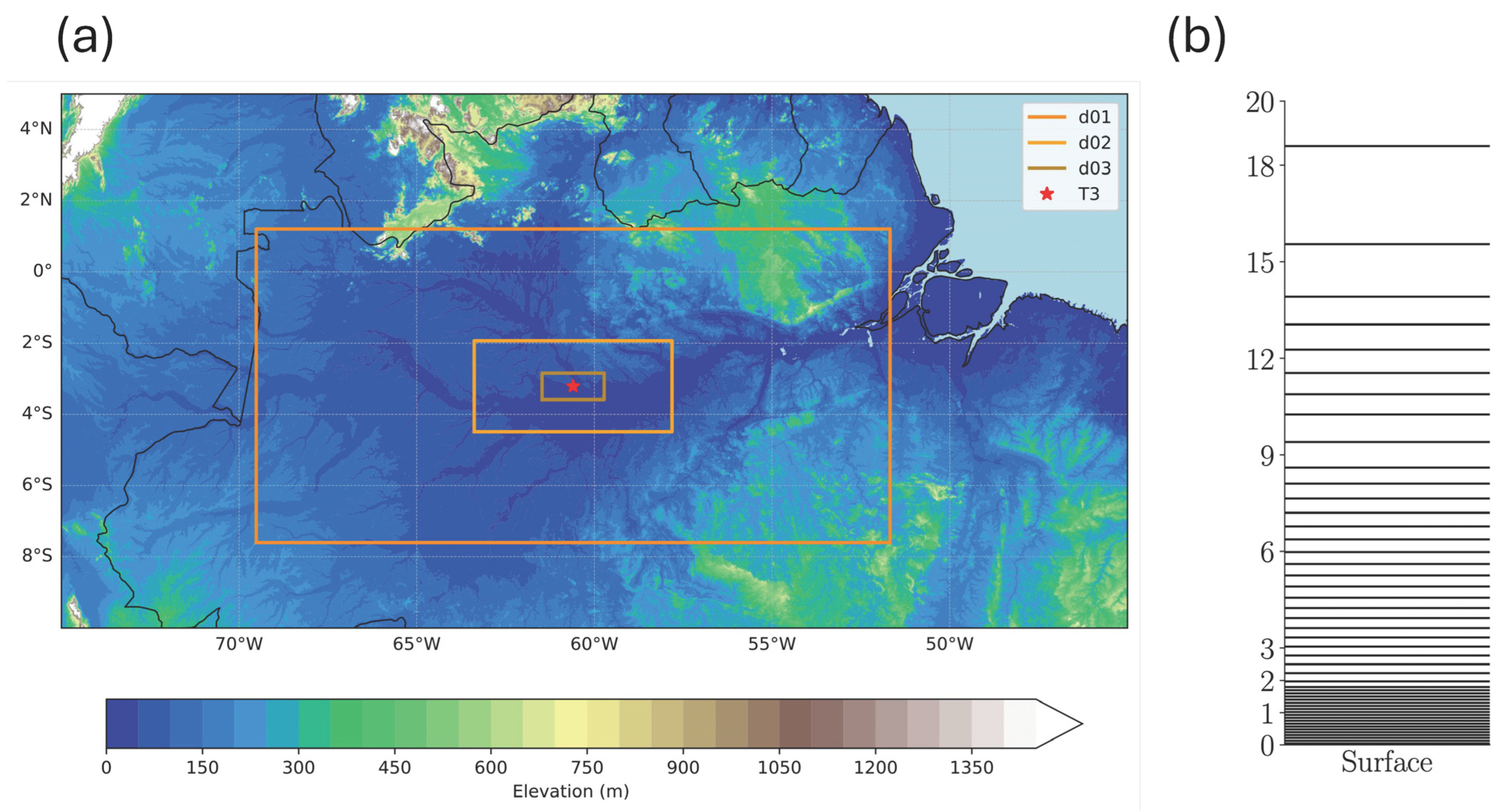
The observational data used in this work were collected in a pasture site named T3 (3.213° S, 60.598° W, 50 m; Figure 1a), which is surrounded by native forest in the Brazilian Central Amazon, situated nearby the intersection of Negro and Solimões rivers in the Manacapuru municipality, Amazonas state, Brazil. The T3 site was the most comprehensively instrumented site of the GoAmazon2014/5 campaign [47]. The facility deployed at the T3 site was composed of the Atmospheric Radiation Measurement (ARM) Mobile Facility One (AMF-1) and the ARM Mobile Aerosol Observing System (MAOS) [48]. The measurements analyzed in this research were related in two official Intensive Operating Periods (IOPs), wet and dry seasons of 2014, respectively, from 15 February to 31 March (IOP1) and from 1 September to 15 October (IOP2) [47].
Figure 1.
(a) Study area showing WRF parent (d01–9km) and nested domains (d02–3 km and d03–1 km) with ETOPO1 terrain height data; and (b) all model vertical levels (y-axis unit is km). The T3 site is indicated by the red star.
The eddy covariance fluxes such as the sensible heat flux (H) and latent heat flux (LE) were collected with the Eddy CORrelation Flux (30ECOR) [49] measurement system 3 m above the ground in 30 min averages. There are no data available for turbulent fluxes during the IOP1 due to instrumental failures, for which the ARM Variational Analysis (VARANAL) [50] data were employed to fill this gap. The environmental structures, i.e., the vertical profiles for the potential temperature (θ), vapor mixing ratio (q), and horizontal wind speed (U) at 2, 8, 11, 14, and 20 local time (LT = GMT-4h), were obtained through radiosonde soundings (SONDEWNPN) [51] launched over the T3 site at regular intervals. The daily cycle of PBLH was estimated using laser ceilometer measurements (CEILPBLHT) [52] as described by Carneiro and Fisch [53]. The ceilometer is considered the best instrument to capture the entire PBLH daily cycle and provides a better comparison with radiosonde-estimated PBLH in both Stable Boundary Layer (SBL) and Convective Boundary Layer (CBL) conditions [53,54]. These observed variables are directly compared to simulations performed within the WRF model using different PBL schemes.
2.2. Model Configuration and Experimental Design
Numerical experiments were performed using the WRF model version 4.2.2 [27]. The model domain consists of three one-way interacting nested grids with a grid spacing of 9 km (d01), 3 km (d02), and 1 km (d03), respectively, centered on the location of the T3 site (Figure 1a). The vertical grid has 50 hybrid sigma-pressure levels. The first 20 levels are distributed within the lowest 2 km of the atmosphere to provide high-resolution vertical grid for PBL processes (Figure 1b), with the first level at 40 m above the surface, and the model top was set at 50 hPa. The integration time-step was set to six times the horizontal resolution (∆t = 6 × ∆x), which was 54 s for d01, 18 s for d02, and 6 s for d03. Table 1 summarizes the model configuration.
Table 1.
Overall experimental setup and model configuration.
All runs started at 00 UTC and were integrated continuously for 72 h. The first 12 h are considered the spin-up time and were discarded from the analysis. An output temporal resolution of 1 h was chosen for a comparison with the observations. The WRF initial (IC) and lateral boundary conditions (LBCs) are from the Global Forecast System (GFS) data from the National Centers for Environmental Prediction (NCEP), which are operational global forecast data available at a 0.5° × 0.5° resolution, and were updated every three hours. The Moderate-resolution Imaging Spectroradiometer (MODIS) [55] land-use and soil category data were employed for land initialization and boundary conditions. The physical parameterization schemes include the four-layer Unified Noah land surface (LS) model [56], the Rapid Radiative Transfer Model for GCMs (RRTMG) [57] to compute both the longwave and shortwave radiances, the Eta-Ferrier microphysics scheme [58], and the New Tiedtke cumulus scheme [59] applied only on the parent domain (d01). The Revised MM5 [60] surface layer (SL) scheme was responsible for calculating the surface fluxes, except when the MYJ, MYNN3, or QNSE PBL schemes are used, since they are tied to their own SL schemes. The present study tested eleven PBL schemes, which are indicated below.
2.3. PBL Schemes
PBL schemes are one-dimensional parameterization schemes developed to handle the vertical subgrid-scale fluxes based on the vertical diffusion equations in the atmospheric column [5,18,27]. The most widely used PBL parameterizations in atmospheric models fall into two main categories: local PBL schemes based on 1.5-order TKE (Turbulent Kinect Energy) closure, which parameterizes turbulence based solely on vertical gradients between adjacent layers. These PBL schemes assume that small-scale eddies dominate—making them suitable for SBL conditions. The second category is the non-local PBL schemes that incorporate transport from distant layers using counter-gradient terms to represent large eddy effects, better capturing convective mixing under unstable conditions, i.e., the CBL [5,6,9,17,61,62]. Table 2 summarizes key details from the eleven PBL parameterization schemes tested in the present study, which are grouped as follows.
Table 2.
Details of tested PBL schemes, such as turbulence closure order, mixing approach, method of PBLH definition, and the threshold value (all taken from their respective references).
Local PBL schemes considered are the Bougeault–Lacarrère (BouLac) [63], GBM [64], UW [65], MYJ [66,67,68], MYNN2.5, and MYNN3 [69,70]. Their main differences are the terms retained in the derivation of TKE equations and the choice of parameter values [71]. Regarding the PBLH definition method, the BouLac, MYJ, and MYNN schemes assume the PBLH as the level where TKE reaches a predefined threshold. On the other hand, the GBM PBL scheme predicts the PBLH using an entrainment closure approach [64], while the UW scheme defines the PBLH as the inversion height between model levels, using a threshold based on the bulk Richardson number (Rib) [65].
The non-local and hybrid PBL schemes considered are the Medium Range Forecast (MRF) [10], YSU [72], Shin and Hong (SH) [15], ACM2 [12,13], and Quasi-Normal-Scale-Elimination (QNSE) [11,73,74]. Both MRF and YSU PBL schemes are similar non-local PBL schemes, while the SH considers a non-local scale-aware approach for the convective PBL [15], the ACM2 uses a hybrid mixing approach that takes a transilient matrix into account to define the mass flux between model layers [12,13], and the QNSE uses a hybrid approach through a local closure with fraction-polynomial fits from the analytical QNSE theory [11,73] and a non-local updraught eddy-mass-flux scheme [74]. In terms of the PBLH definition, they have particular methods based on the buoyancy profile, bulk Richardson number, TKE based, etc. (Table 2). These pronounced differences among PBLH definition methods may introduce uncertainty [22]. One solution to ensure a common PBLH definition method is using the bulk Richardson method to diagnose the PBLH, as given by the following equation:
where is the acceleration due to gravity; and are the virtual potential temperatures at the surface and at the boundary-layer top, respectively; is the boundary layer depth; and and are the wind speed components at the boundary layer top. The PBLH is defined as the height at which first reaches a critical Richardson number () defined as 0.25 [75]. In the present study, the calculation was performed by using the vertical profiles of temperature, moisture, and wind speed from WRF output files.
2.4. Model Evaluation
The observational datasets described in Section 2.1 were employed to assess the performance of numerical experiments. All simulated variables considered in the evaluation were extracted from the T3 site location on the d03 1-km domain and directly compared with in situ observations [49,50,51,52]. The daily cycle variations over the Central Amazon Basin are significant; then, the performance of the simulated nocturnal SBL and diurnal CBL must be evaluated separately [39,53]. The model evaluation begins by the identification of the best PBL scheme to reproduce the hourly PBLH during both nighttime (19-5 LT) and daytime (6-18 LT) periods. Taylor diagrams were employed for the PBLH analysis, which simultaneously displays three statistical parameters: the Pearson correlation coefficient (R), the standard deviation (σ), and the Centered Root Mean Square Error (CRMSE), which are displayed along with Taylor Skill Score (TSS) [76]. A detailed description of each statistical metric can be found in Table A1 (see Appendix A). The vertical PBL structure is evaluated using radiosonde soundings, and turbulent heat fluxes are compared to PBLH to investigate energy partitioning and surface–atmosphere coupling. The spatial distributions of PBLH during daytime and nighttime are investigated qualitatively to identify the impact of different PBL schemes over the Central Amazon Basin heterogeneities (i.e., rivers and water bodies, forecast canopy, and urban areas). It is important to note that, at the 1-km grid spacing, boundary-layer eddies are partially resolved while parameterized turbulence remains active. This scale interaction may influence the relative performance of PBL schemes.
3. Results
3.1. Performance Evaluation Outcomes
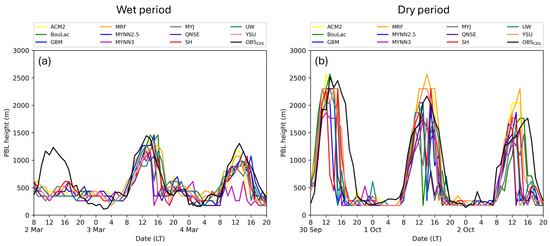
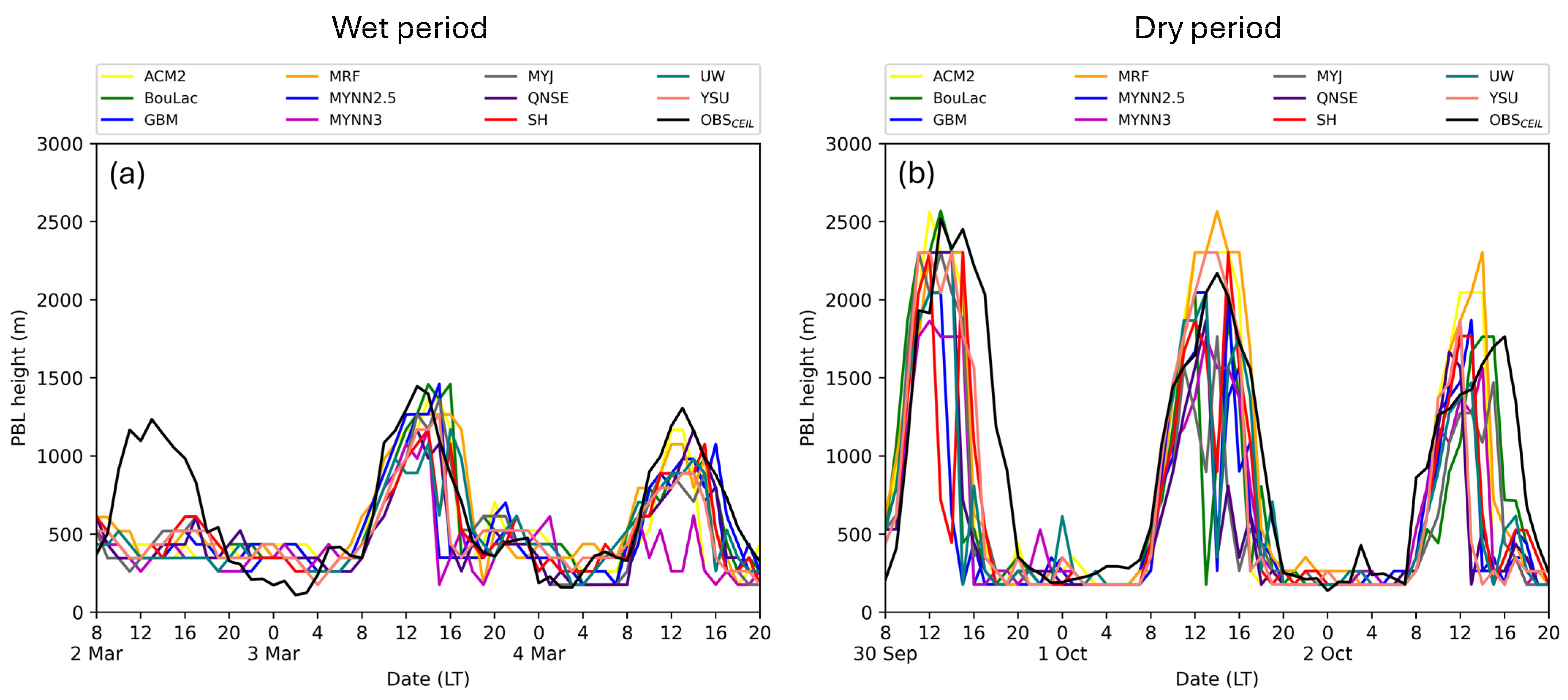
The PBLH is critical for many applications in atmospheric science [22,77], in which PBL schemes are responsible for estimating this key variable within NWP models. Figure 2 shows the observed and diagnosed PBLH from PBL schemes during both periods. The observed PBLH over the T3 site (pasture) shows a characteristic of a deeper PBL during the day and shallower at night, which is related to the daily cycle conditions [53]. The comparison between the observed PBLH during wet (Figure 2a) and dry (Figure 2b) periods reveals that a deeper PBL is formed during the daytime in the dry period with the PBLH reaching ~2500 m, while a maximum PBLH is around 1500 m during the wet period. The fact that a lower PBLH is observed during the wet period is associated with the combination of a weak stable nocturnal PBL and lower H flux, which causes a slow erosion of the SBL and consequently impacts PBL growth. On the other hand, the greater stability of the nocturnal PBL and the earlier occurrence of positive radiation balance and H flux result in the earlier erosion of the SBL during the dry period. This generates rapid PBL growth, a prolonged CBL phase, and consequently a higher PBLH [53]. The PBL schemes were unable to reproduce the PBLH daily cycle on March 2 (Figure 2a). This behavior may indicate that the 12 h spin-up period is insufficient for the wet period, and/or reflect sensitivity to initial conditions and land-atmosphere adjustment processes under moist convective environments.
Figure 2.
Comparison between observed and diagnosed PBLH at T3 site during (a) wet and (b) dry periods.
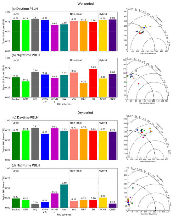
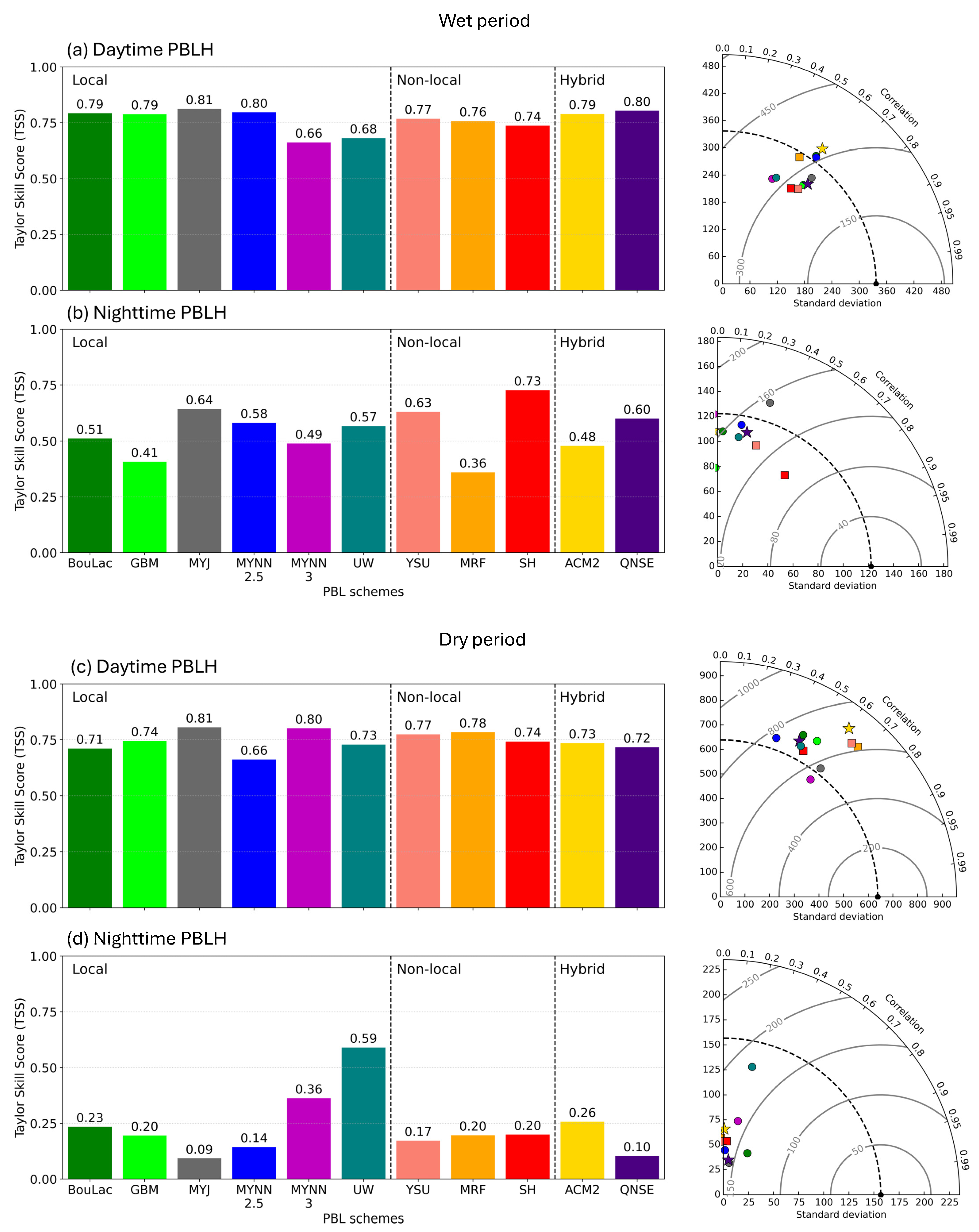
We start our evaluation by considering the performance of the eleven PBL parameterization schemes in terms of reproducing the observed ceilometer-estimated PBLH [52]. This is demonstrated through the Taylor Skill Score (TSS) bar charts and Taylor diagrams presented in Figure 3 that summarizes how well the PBL schemes reproduced the observed PBLH during daytime and nighttime and under wet and dry conditions, respectively. The analysis reveals substantial variability among the PBL schemes, strongly modulated by both the season (wet vs. dry period) and diurnal cycle (daytime vs. nighttime). In general, PBL schemes performed better during the wet period (Figure 3a,b), whereas nighttime conditions—particularly during the dry period (Figure 3d)—posed the greatest challenge. Regarding the performance of PBL schemes by category—local, non-local, and hybrid—all of them performed similarly during the daytime PBLH for both wet and dry periods, while non-local (local) PBL schemes were better at night in the wet (dry) period. During the wet period (Figure 3a,b), daytime simulations exhibited a lower CRMSE (≈300 m; Figure 3a), while nighttime variability was significantly lower (CRMSE ≈ 80–160 m; Figure 3b). Daytime TSS values ranged from 0.66 (MYNN3) to 0.81 (MYJ), with the MYJ scheme showing the highest skill.
Figure 3.
Taylor Skill Score bar chart (left) and Taylor diagram (right) for hourly PBLH during the (a) daytime and (b) nighttime in the wet period and during the (c) daytime and (d) nighttime in the dry period. Standard deviation (dashed black line) and CRMSE (filled grey lines) are given in meters. The ordinate axis of the Taylor diagram shares its identity with the abscissa. Local PBL schemes are indicated by circles, non-local ones by squares, and hybrid ones by stars in the Taylor diagrams.
At night, the SH scheme had the best skill (TSS = 0.73). SH had the highest TSS based on the daily average (=0.74), followed by MYJ ( = 0.73), YSU, and QNSE ( = 0.70). Overall model performance worsened during the dry period (Figure 3c,d)—especially at night (Figure 3d). Most PBL schemes exhibited higher standard deviation (σ ≈ 500–800 m) during the daytime conditions (Figure 3c) compared to the wet period. MYJ achieved the highest daytime TSS (=0.81), while UW exhibited the best nighttime performance (TSS = 0.59). UW had the highest TSS based on the daily average (=0.66). The lower skill at night during the dry period is possibly associated with the greater stability of the observed SBL and coarser model vertical resolution.
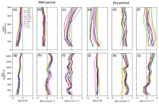
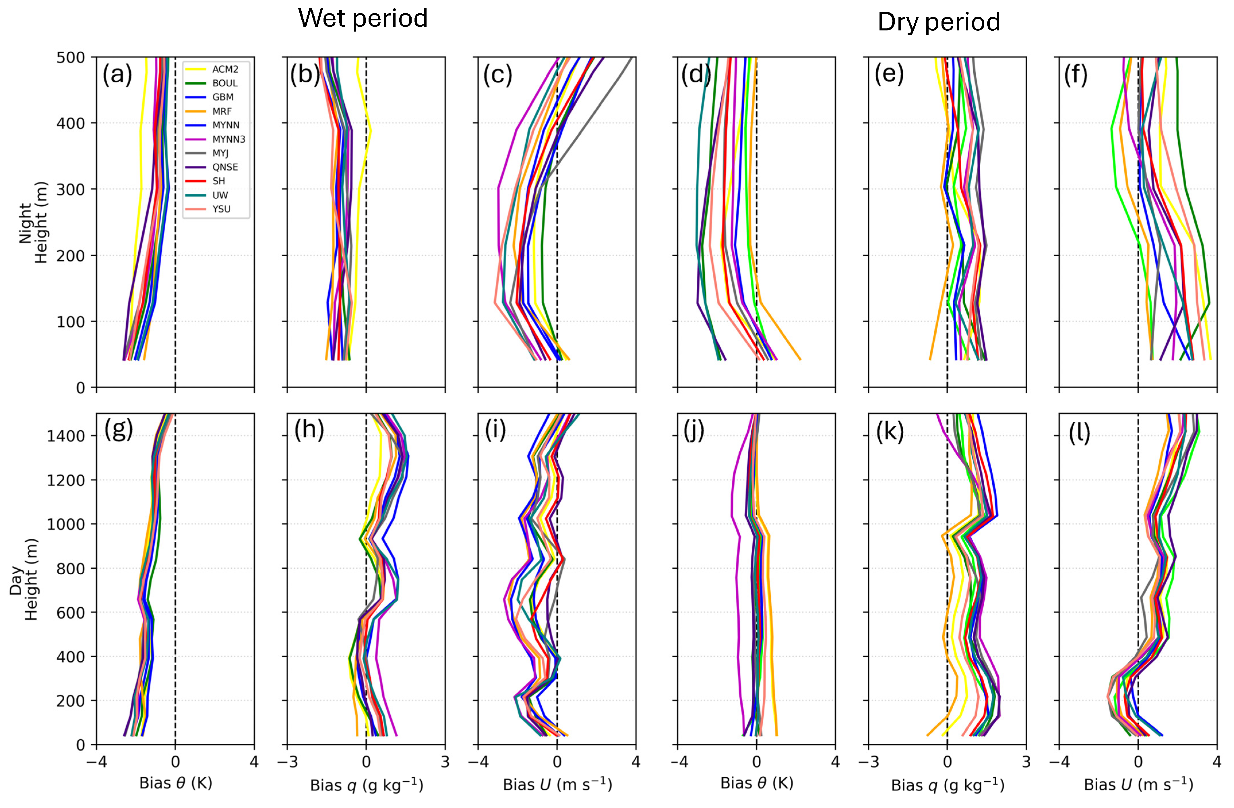
Figure 4 shows the bias vertical profiles of averaged θ, q, and U at daytime and nighttime during wet and dry periods. Nighttime profiles of θ show a cold bias during both periods with greater variability among them during the dry period (Figure 4a,d). The opposite is seen when comparing q profiles from wet (dry bias) and dry (wet bias) periods (Figure 4b,e). Also, greater variability and opposite behavior are observed among PBL schemes for U profiles during the nighttime (Figure 4c,f). The greater variability observed in the nighttime profiles during the dry period helps explain the lower performance of PBLH associated with struggle to simulate the high stability and nocturnal low-level jet characteristic of the Amazonian nocturnal boundary layer. This suggests that the vertical grid resolution used may be insufficient to adequately resolving the strong gradients characteristic of the SBL. In addition to vertical resolution, known deficiencies in turbulence parametrizations under stable conditions such as the representation of intermittency and weak mixing likely contribute to the reduced performance during night. Greater differences arise from 20 LT profiles (not shown), possibly due to model difficulties in reproducing the complex transition from day to night [53].
Figure 4.
Bias vertical profiles of potential temperature (), specific humidity (), and wind speed () averaged for nighttime (2 and 20 LT) during the wet (a–c) and dry periods (d–f) and averaged for daytime (8, 11, and 14 LT) during wet (g–i), and dry periods (j–l).
During the daytime, PBL schemes exhibit a consistent cold bias in the lower 1000 m in the wet case (Figure 4g). This cold bias indicates that the PBL schemes struggle to maintain the observed lapse rate, effectively trapping energy near the surface or diluting it through an incorrectly mixed volume. On the other hand, most PBL schemes show near-zero bias at daytime during the dry period (Figure 4j), suggesting that they can better reproduce it compared to the wet period. The greatest differences are observed in the bias profiles at 11 LT (not shown), which indicates that the model has difficulty eroding the nocturnal SBL, thus presenting differences in the morning transition stage. The q profiles show a slight wet bias during the daytime in the wet period. This suggests that several schemes may be overestimating vertical moisture transport (Figure 4h). This behavior is more pronounced in the dry period, when PBL schemes clearly show a wet bias (Figure 4k). Wind speed profiles show an underestimation during the wet period (Figure 4i). In contrast, they underestimated near the surface and overestimated aloft during the dry period (Figure 4l). MYJ shows the lowest bias at mid-levels, which support its better performance for daytime PBLH. The use of a standardized bulk Richardson diagnosis for PBLH across all PBL schemes reveals that even when the diagnostic PBLH method is identical, the underlying differences in the vertical transport of heat and momentum lead to significant variations in the diagnosed PBLH. This confirms that errors in the simulated PBLH are rooted in the internal physics of turbulent mixing and its interaction with the surface, rather than being an artifact of the different diagnostic definitions used by each PBL scheme. Hara [78] demonstrated that inadequate vertical resolution can hinder the accurate prediction of the vertical structure, consequently impacting the PBLH definition. In short, our analysis suggests that a high-resolution vertical grid is necessary to accurately reproduce the thermodynamic and dynamic vertical structures of the observed Amazon SBL.
3.2. Energy Partitioning and Surface–Atmosphere Coupling
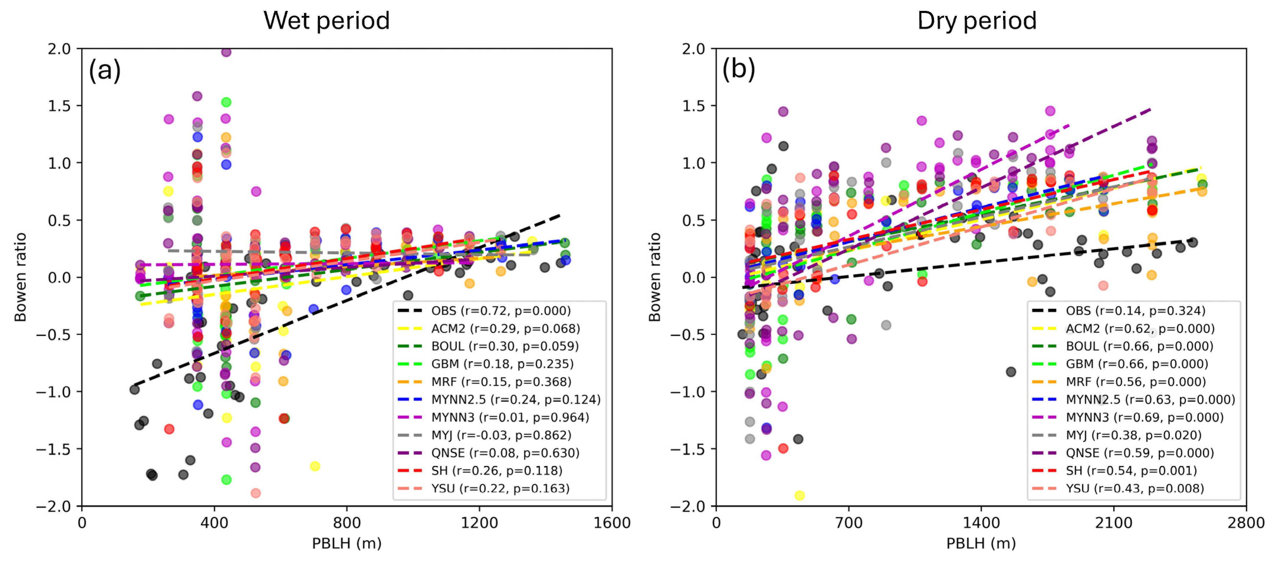
Figure 5 shows the relationship between the Bowen ratio (i.e., the ratio H/LE) and PBLH from the observed and modeled data during wet and dry periods. The observations are characterized by generally low Bowen ratios, reflecting the dominance of LE in the energy-limited regime characteristic of the wet period (Figure 5a).
Figure 5.
Scatter plots of Bowen ratio (B = H/LE) versus PBLH during (a) wet and (b) dry periods. Only data with |LE| > 5 W·m−2 are included. The R and p-value are shown in the legend.
Despite the relatively low Bowen ratios, the observed PBLH frequently reaches depths of 1000–1500 m, indicating a strong sensitivity of PBL growth to variations in surface energy partitioning even when sensible heat fluxes are modest. However, under these moist conditions, boundary-layer development is also strongly influenced by cloud cover, entrainment processes, and large-scale atmospheric forcing, which can reduce the direct dependence of PBLH on surface fluxes alone. In contrast, the WRF simulations show a markedly weaker response. The slope of the Bowen ratio–PBLH relationship is substantially flatter in the models, indicating that the simulated PBLH is largely insensitive to changes in surface energy partitioning during the wet period. This weak coupling suggests that, under moist conditions, the simulated PBL growth is controlled more by parameterized entrainment and stability constraints than by surface flux variability.
During the dry period (Figure 5b), surface forcing transitions to a more water-limited regime, and Bowen ratios increase substantially. In this regime, the observed data show a weak linear relationship between the Bowen ratio and the PBLH (r = 0.14, p = 0.32). This reduced sensitivity likely reflects the influence of residual layers, advection, and the temporal evolution of the boundary layer, whereby PBLH is not solely controlled by instantaneous surface fluxes but also by its prior development. In addition, limitations in aerosol-based PBLH detection under dry conditions may contribute to decouple the observed PBLH from instantaneous surface fluxes. In contrast, all eleven PBL schemes exhibit strong and statistically significant linear relationships between the Bowen ratio and PBLH during the dry period. This behavior may indicate an over-reliance on local surface forcing, with insufficient representation of entrainment and non-local processes that contribute to the deeper PBL growth observed in reality. As a result, the simulated PBLH remains lower, clustering around 1200–1400 m for Bowen ratios, at which observations frequently exceed 2000 m.
3.3. Spatial Distribution of PBLH over the Central Amazon Basin
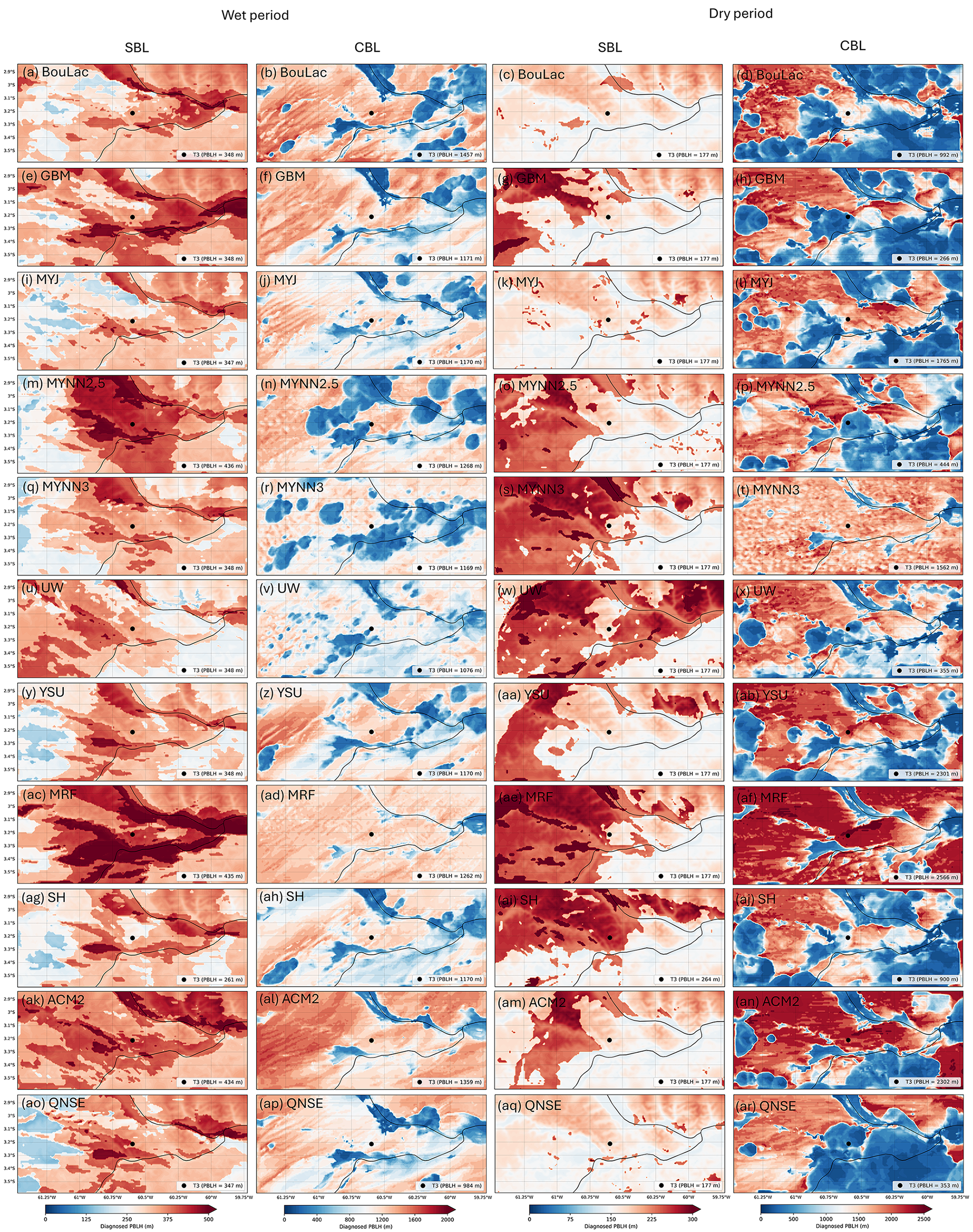
Modeling tools can be useful to investigate, for instance, the development of PBLH over remote areas in the absence of observational data related to difficulties in making continuous measurements [79]. Moreover, PBLH observations mostly rely on single-point measurements (e.g., radiosonde, lidar, and ceilometer) since observations providing the spatial distribution of PBLH are scarce due to the spatial and temporal limitations of current instruments [80,81]. Figure 6 shows the spatial fields of the diagnosed PBLH at 2 LT (SBL) and 14 LT (CBL) over the Central Amazon Basin during the wet (3 March 2014) and dry (1 October 2014) conditions. There are no observations to conduct a spatial comparison against the model data; however, the spatial analysis can qualitatively reveal some interesting features about the impact of the PBL schemes over the region. During the wet period, all PBL schemes show an opposite behavior between land and river areas, as well as day and night. Low (high) PBLH is diagnosed over land, while high (low) PBLH is diagnosed over rivers during the night (day). The Central Amazon Basin exhibits a thermal contrast between the rainforest and rivers/waterbodies at night, where the Negro and Solimões rivers retain heat more efficiently and cool more slowly than the surrounding forest, resulting in warmer surface at night. All PBL schemes simulated higher LE and H over the water compared to the cooling forest (not shown), which explains a deeper PBL over the rivers. Also, high turbulence occurs over the Manaus megacity (~3.1° S, 60° W), where PBL schemes simulate higher u* (friction velocity; not shown), possibly due to urban roughness and the urban heat island effect, yielding a deeper PBL compared to surrounding forested areas. The observed PBLH is 110 m on T3 site at 2 LT, while all PBL schemes show values above 250 m. In contrast to the nighttime, the thermal gradient reverses during the daytime, with the forest heating more rapidly and generating stronger heat fluxes, while the rivers remain relatively cooler.
Figure 6.
Spatial distributions of PBLH during SBL (2 LT) and CBL (14 LT) stages from wet (3 March 2014) and dry (1 October 2014) periods. The black dot is the T3 location, and the black line represents the rivers in the region. PBL schemes are row-biased. PBLH retrieved at the T3 location is indicated in the lower right corner.
The spatial fields of u*, LE, and H over rivers (not shown) revealed a decrease during the day, which suggests the suppression of mechanical and thermal turbulence leading to a reduction in the PBLH as seen in the PBLH distributions. MRF appears to be less sensitive to this thermal gradient during the day, since it shows higher PBLH even over the rivers (Figure 6ad). Non-local PBL schemes tend to produce slightly deeper PBL over the region compared to local ones, although a point-comparison at the T3 site indicates that some local PBL schemes produced deeper PBL (e.g., MYNN2.5 vs. SH). The observed PBLH on T3 site is 1397 m at 14 LT, which most PBL schemes underestimated, except BouLac (=1457 m). ACM2 had the best agreement at this time, showing 1359 m. Additionally, local PBL schemes (e.g., Figure 6b,f,j,n,r,v) reveal larger regions of low PBLH, resembling “bubbles”, which are associated with convective activity.
In the dry period, the river effect reverses during the nighttime where most PBL schemes show a lower PBLH over rivers compared to land. Some PBL schemes still exhibit higher PBLH over rivers (e.g., Figure 6o,s,w). The spatial distribution of turbulent fluxes reveals the thermal gradient observed during the wet period (not shown); however, the diagnosed PBLH behaves different. Possibly, it is related to differences in shear and buoyancy. PBL schemes showed higher PBLH over Manaus as expected due to increased turbulence. The observed PBLH on T3 at 2 LT is 224 m, which SH closely reproduced (264 m; Figure 6ai) and other PBL schemes underestimated (PBLH = 177 m). The daytime PBL during the dry period shows a deeper depth compared to the wet period, particularly from simulations using non-local and hybrid PBL schemes (e.g., Figure 6af,an) when compared to local ones. Similarly to the wet period, the daytime PBL is deeper over land and shallower over rivers. The rivers act as sinks for vertical mixing; however, it seems to curiously not impact MYNN3 (Figure 6t). The observed PBLH on T3 is 2170 m, for which PBL schemes such as YSU and ACM2 showed closer values (~2300 m). The analysis also shows how the horizontal variability impacts the grid-point comparison. For example, although PBL schemes such as BouLac (Figure 6d), GBM (Figure 6h), and MYNN2.5 (Figure 6p) reproduce general behavior, they showed a shallower PBL on the T3 site.
4. Discussion and Conclusions
This study evaluated the performance of eleven PBL parameterization schemes within the WRF model over the Central Amazon Basin, leveraging high-resolution (1 km) simulations and comprehensive observations from the GoAmazon2014/5 campaign [47]. The analysis focused on contrasting wet and dry periods and explicitly examined daytime convective and nighttime stable boundary layer regimes. The overarching objective was to identify which PBL schemes most effectively reproduce the observed PBLH and investigate their impact on the spatial distribution of the PBLH over the region.
The first research question—whether a preferred PBL scheme exists for each period—can be answered affirmatively, but with strong dependence on the stability regime. SH showed the highest overall performance among the tested configurations during the wet period, especially at night. Some PBL schemes, such as locals MYJ and MYNN2.5, non-locals YSU and MRF, and hybrids ACM2 and QNSE, showed comparable skill or slightly better skill than SH during the daytime PBL but performed worse at night. Regarding the dry season, both local MYJ and MYNN3 PBL schemes showed the best skills during the daytime PBL, while local UW had the best overall performance particularly due to its superior skill at night. In general, most PBL schemes can reproduce the daytime PBL with high skill (TSS > 0.70) in both periods. On the other hand, more variability in skill is observed at night especially during the dry period where most PBL schemes showed lower skill (TSS < 0.50). This suggests that most PBL schemes struggle to reproduce the well-stable nocturnal PBL observed during the dry period in the Amazon region. These results corroborate previous studies investigating the impact of PBL schemes to reproduce the observed PBLH in the region [39,44,45]. Although the PBLH diagnostics provide a fair comparison between PBL schemes, we do not consider the advantage from their built-in PBLH methods; if so, MYNN2.5 would have the best skill (TSS = 0.87) at night during the dry period. In addition, this study lies within the gray-zone (1 km grid spacing), where turbulent eddies are partially resolved. The performance of PBL schemes may therefore be influenced by interactions between resolved and parameterized turbulence. The relatively consistent performance of the SH scheme may be partially associated with its scale-aware non-local closure.
Regarding the second question about the impact of PBL schemes on reproducing the observed conditions near-surface and within the PBL, a systematic cold bias was identified at night during both periods. A dry (wet) bias is observed during the day in the wet (dry) period from most PBL schemes. This is likely associated with inefficient vertical mixing and wind speed depiction, consistent with bias in wind speed profiles [78]. This suggests that the parameterized entrainment within PBL schemes is insufficiently sensitive to buoyancy forcing under the high-energy conditions compared to observations. Furthermore, while the model vertical configuration (Figure 1b) appears sufficient for capturing the deeper CBL, the 40 m height of the first model level and adopted vertical distribution may be too coarse for the shallow Amazonian SBL. As demonstrated by Hara [78], vertical discretization significantly impacts the prediction of inversion heights and can lead to artificial numerical entrainment. Consequently, the lower model skill during nocturnal periods likely reflects the difficulty of resolving sharp near-surface gradients and low-level jets.
The third research question explored the regional impact of PBL schemes on the spatial distribution of the PBLH. The qualitative analysis revealed that the choice of PBL scheme alters the diagnosed PBLH across the Central Amazon Basin. The simulations successfully captured the river effect, where the Negro and Solimões rivers remain relatively warmer during the nighttime due to their higher heat capacity, yielding a deeper PBL over water, while the forest undergoes rapid radiative cooling, resulting in a shallower PBL. Furthermore, PBL schemes simulated a deeper PBLH over the Manaus urban area due to enhanced mechanical and thermal forcing possibly associated with surface roughness and urban heat island effects. Also, the spatial fields underscore the limitations of grid-point comparisons, whereby PBL schemes may realistically reproduce the large-scale spatial structure of PBL depth while underestimating PBLH at the specific location of observation. These results are particularly important for pollutant dispersion and air quality studies over the region, since the mixing and dispersion of chemicals occur within the PBL [22,24,26,82]. In addition, the results contribute to highlight the importance of developing observational products [80,81] that could provide a means to verify the spatial distribution of the PBLH over regions with such horizontal heterogeneities. Further investigation of the simulated spatial distribution of PBLH is necessary to better understand its fidelity compared to the reality, particularly at night.
Despite these findings, certain uncertainties remain. The presented model performance combines the predictability of three-day periods from the wet and dry seasons, the accuracy of NCEP-GFS data used as IC and LBC, the WRF model skill, and uncertainties from PBL scheme formulations. We did not investigate how changing the IC and LBC source or lead time initialization impact our results. This must be tested in future studies, along with a long-term period to improve statistical robustness since the results reflects case-study findings and may not fully capture the statistical variability of boundary-layer behavior over the region. In conclusion, while WRF reasonably captures the horizontal heterogeneity of the Central Amazon landscape, improving the representation of the vertical interface physics is critical to achieving accurate tropical PBL simulations. Additionally, we strongly recommend increasing the vertical grid resolution.
Author Contributions
J.A.M.: writing—original draft, writing—review and editing, conceptualization, investigation, methodology, software, validation, data curation, formal analysis. R.C.: writing—review and editing, methodology development, interpretation of results, data curation. C.K.B.: writing—review and editing, methodology development, interpretation of results, formal analysis. S.I.-E.: writing—review and editing, methodology development, validation, interpretation of results. J.A.A.: writing—review and editing, conceptualization, methodology, investigation, supervision. G.F.: writing—review and editing, conceptualization, methodology, supervision. D.L.H.: writing—review and editing, funding acquisition, project administration, and supervision. All authors have read and agreed to the published version of the manuscript.
Funding
This study was financed in part by the Coordenação de Aperfeiçoamento de Pessoal de Nível Superior—Brasil (CAPES)—Finance Code 001. José Antonio Mantovani acknowledges the National Council for Scientific and Technological Development (CNPq) for his grant (GM/GD 131094/2020-3).
Data Availability Statement
The ARM datasets used for this study can be found online in the ARM GoAmazon2014/5 database at https://www.arm.gov/research/campaigns/amf2014goamazon (accessed on 18 March 2025). The WRF model outputs are available upon request.
Acknowledgments
We acknowledge the ARM team for their efforts in producing and maintaining the GoAmazon2014/5 datasets. We also acknowledge the National Laboratory for Scientific Computing (LNCC/MCTI, Brazil) for providing computational resources of the Santos Dumont (SDumont) supercomputer, which have contributed to the research results reported in this paper.
Conflicts of Interest
The authors declare no conflicts of interest.
Appendix A
Statistical metrics used in this study.
Table A1.
Statistical metrics considered in the model evaluation.
References
- Olafsson, H.; Bao, J.W. Uncertainties in Numerical Weather Prediction; Elsevier: Amsterdam, The Netherlands, 2021. [Google Scholar] [CrossRef] [Scilit]
- Stensrud, D.J. Parameterization Schemes: Keys to Understanding Numerical Weather Prediction Models; Cambridge University Press: Cambridge, UK, 2007. [Google Scholar] [CrossRef] [Scilit]
- Dzebre, D.E.; Adaramola, M.S. A preliminary sensitivity study of Planetary Boundary Layer parameterisation schemes in the weather research and forecasting model to surface winds in coastal Ghana. Renew. Energy 2020, 146, 66–86. [Google Scholar] [CrossRef] [Scilit]
- Zhang, X. Chapter 7—Subgrid turbulence mixing. In Uncertainties in Numerical Weather Prediction; Olafsson, H., Bao, J.W., Eds.; Elsevier: Amsterdam, The Netherlands, 2021; pp. 205–227. [Google Scholar] [CrossRef] [Scilit]
- Stull, R.B. An Introduction to Boundary Layer Meteorology; Springer Science & Business Media: Berlin/Heidelberg, Germany, 1988; Volume 13. [Google Scholar] [CrossRef] [Scilit]
- Cohen, A.E.; Cavallo, S.M.; Coniglio, M.C.; Brooks, H.E. A review of planetary boundary layer parameterization schemes and their sensitivity in simulating southeastern US cold season severe weather environments. Weather Forecast. 2015, 30, 591–612. [Google Scholar] [CrossRef] [Scilit]
- Louis, J.F. A parametric model of vertical eddy fluxes in the atmosphere. Bound.-Layer Meteorol. 1979, 17, 187–202. [Google Scholar] [CrossRef] [Scilit]
- Mellor, G.L.; Yamada, T. Development of a turbulence closure model for geophysical fluid problems. Rev. Geophys. 1982, 20, 851–875. [Google Scholar] [CrossRef] [Scilit]
- Troen, I.B.; Mahrt, L. A simple model of the atmospheric boundary layer; sensitivity to surface evaporation. Bound.-Layer Meteorol. 1986, 37, 129–148. [Google Scholar] [CrossRef] [Scilit]
- Hong, S.Y.; Pan, H.L. Nonlocal boundary layer vertical diffusion in a medium-range forecast model. Mon. Weather Rev. 1996, 124, 2322–2339. [Google Scholar] [CrossRef] [Scilit]
- Sukoriansky, S.; Galperin, B.; Perov, V. Application of a new spectral theory of stably stratified turbulence to the atmospheric boundary layer over sea ice. Bound.-Layer Meteorol. 2005, 117, 231–257. [Google Scholar] [CrossRef] [Scilit]
- Pleim, J.E. A combined local and nonlocal closure model for the atmospheric boundary layer. Part I: Model description and testing. J. Appl. Meteorol. Climatol. 2007, 46, 1383–1395. [Google Scholar] [CrossRef] [Scilit]
- Pleim, J.E. A combined local and nonlocal closure model for the atmospheric boundary layer. Part II: Application and evaluation in a mesoscale meteorological model. J. Appl. Meteorol. Climatol. 2007, 46, 1396–1409. [Google Scholar] [CrossRef] [Scilit]
- Angevine, W.M.; Jiang, H.; Mauritsen, T. Performance of an eddy diffusivity–mass flux scheme for shallow cumulus boundary layers. Mon. Weather Rev. 2010, 138, 2895–2912. [Google Scholar] [CrossRef] [Scilit]
- Shin, H.H.; Hong, S.Y. Representation of the subgrid-scale turbulent transport in convective boundary layers at gray-zone resolutions. Mon. Weather Rev. 2015, 143, 250–271. [Google Scholar] [CrossRef] [Scilit]
- Olson, J.B.; Kenyon, J.S.; Angevine, W.; Brown, J.M.; Pagowski, M.; Sušelj, K. A Description of the MYNN-EDMF Scheme and the Coupling to Other Components in WRF–ARW; National Oceanic and Atmospheric Administration (NOAA): Washington, DC, USA, 2019. [CrossRef]
- Zhang, C.; Wang, Y.; Xue, M. Evaluation of an E–ε and three other boundary layer parameterization schemes in the WRF model over the Southeast Pacific and the Southern Great Plains. Mon. Weather Rev. 2020, 148, 1121–1145. [Google Scholar] [CrossRef] [Scilit]
- Shin, H.H.; Hong, S.Y. Intercomparison of planetary boundary-layer parametrizations in the WRF model for a single day from CASES-99. Bound.-Layer Meteorol. 2011, 139, 261–281. [Google Scholar] [CrossRef] [Scilit]
- Wang, W.; Shen, X.; Huang, W. A comparison of boundary-layer characteristics simulated using different parametrization schemes. Bound.-Layer Meteorol. 2016, 161, 375–403. [Google Scholar] [CrossRef] [Scilit]
- Moya-Álvarez, A.S.; Estevan, R.; Kumar, S.; Rojas, J.L.F.; Ticse, J.J.; Martínez-Castro, D.; Silva, Y. Influence of PBL parameterization schemes in WRF_ARW model on short-range precipitation’s forecasts in the complex orography of Peruvian Central Andes. Atmos. Res. 2020, 233, 104708. [Google Scholar] [CrossRef] [Scilit]
- He, J.; Chen, D.; Gu, Y.; Jia, H.; Zhong, K.; Kang, Y. Evaluation of planetary boundary layer schemes in WRF model for simulating sea-land breeze in Shanghai, China. Atmos. Res. 2022, 278, 106337. [Google Scholar] [CrossRef] [Scilit]
- Jia, W.; Zhang, X. The role of the planetary boundary layer parameterization schemes on the meteorological and aerosol pollution simulations: A review. Atmos. Res. 2020, 239, 104890. [Google Scholar] [CrossRef] [Scilit]
- De Lange, A.; Naidoo, M.; Garland, R.M.; Dyson, L.L. Sensitivity of meteorological variables on planetary boundary layer parameterization schemes in the WRF-ARW model. Atmos. Res. 2021, 247, 105214. [Google Scholar] [CrossRef] [Scilit]
- De Lange, A.; Naidoo, M.; Garland, R.M.; Dyson, L.L. The sensitivity of simulated surface-level pollution concentrations to WRF-ARW-model PBL parameterisation schemes over the Highveld of South Africa. Atmos. Res. 2021, 254, 105517. [Google Scholar] [CrossRef] [Scilit]
- Jo, H.Y.; Lee, H.J.; Jo, Y.J.; Heo, G.; Lee, M.; Kim, J.A.; Park, M.S.; Lee, T.; Kim, S.W.; Lee, Y.H.; et al. A case study of heavy PM2.5 secondary formation by N2O5 nocturnal chemistry in Seoul, Korea in January 2018: Model performance and error analysis. Atmos. Res. 2022, 266, 105951. [Google Scholar] [CrossRef] [Scilit]
- Yang, J.; Tang, Y.; Han, S.; Liu, J.; Yang, X.; Hao, J. Evaluation and improvement study of the Planetary Boundary-Layer schemes during a high PM2. 5 episode in a core city of BTH region, China. Sci. Total Environ. 2021, 765, 142756. [Google Scholar] [CrossRef] [Scilit] [PubMed]
- Jensen, A.A.; Gill, D.O.; Powers, J.G.; Duda, M.G. A Description of the Advanced Research WRF Model Version 4.3; No. NCAR/TN-556+STR; National Center for Atmospheric Research: Boulder, CO, USA, 2021. [Google Scholar] [CrossRef]
- Hariprasad, K.B.R.R.; Srinivas, C.V.; Singh, A.B.; Rao, S.V.B.; Baskaran, R.; Venkatraman, B. Numerical simulation and intercomparison of boundary layer structure with different PBL schemes in WRF using experimental observations at a tropical site. Atmos. Res. 2014, 145, 27–44. [Google Scholar] [CrossRef] [Scilit]
- Banks, R.F.; Tiana-Alsina, J.; Baldasano, J.M.; Rocadenbosch, F.; Papayannis, A.; Solomos, S.; Tzanis, C.G. Sensitivity of boundary-layer variables to PBL schemes in the WRF model based on surface meteorological observations, lidar, and radiosondes during the HygrA-CD campaign. Atmos. Res. 2016, 176, 185–201. [Google Scholar] [CrossRef] [Scilit]
- Avolio, E.; Federico, S.; Miglietta, M.M.; Feudo, T.L.; Calidonna, C.R.; Sempreviva, A.M. Sensitivity analysis of WRF model PBL schemes in simulating boundary-layer variables in southern Italy: An experimental campaign. Atmos. Res. 2017, 192, 58–71. [Google Scholar] [CrossRef] [Scilit]
- Tymvios, F.; Charalambous, D.; Michaelides, S.; Lelieveld, J. Intercomparison of boundary layer parameterizations for summer conditions in the eastern Mediterranean island of Cyprus using the WRF-ARW model. Atmos. Res. 2018, 208, 45–59. [Google Scholar] [CrossRef] [Scilit]
- Xu, L.; Liu, H.; Du, Q.; Xu, X. The assessment of the planetary boundary layer schemes in WRF over the central Tibetan Plateau. Atmos. Res. 2019, 230, 104644. [Google Scholar] [CrossRef] [Scilit]
- Gholami, S.; Ghader, S.; Khaleghi-Zavareh, H.; Ghafarian, P. Sensitivity of WRF-simulated 10 m wind over the Persian Gulf to different boundary conditions and PBL parameterization schemes. Atmos. Res. 2021, 247, 105147. [Google Scholar] [CrossRef] [Scilit]
- Sathyanadh, A.; Prabha, T.V.; Chowdhuri, S.; Balaji, B.; Resmi, E.A.; Karipot, A. Evaluation of PBL parameterization schemes against direct observations during a land depression over Central India. Theor. Appl. Climatol. 2021, 144, 253–271. [Google Scholar] [CrossRef] [Scilit]
- Falasca, S.; Gandolfi, I.; Argentini, S.; Barnaba, F.; Casasanta, G.; Di Liberto, L.; Petenko, I.; Curci, G. Sensitivity of near-surface meteorology to PBL schemes in WRF simulations in a port-industrial area with complex terrain. Atmos. Res. 2021, 264, 105824. [Google Scholar] [CrossRef] [Scilit]
- Malečić, B.; Prtenjak, M.T.; Horvath, K.; Jelić, D.; Jurković, P.M.; Ćorko, K.; Mahović, N.S. Performance of HAILCAST and the Lightning Potential Index in simulating hailstorms in Croatia in a mesoscale model–Sensitivity to the PBL and microphysics parameterization schemes. Atmos. Res. 2022, 272, 106143. [Google Scholar] [CrossRef] [Scilit]
- Njuki, S.M.; Mannaerts, C.M.; Su, Z. Influence of planetary boundary layer (PBL) parameterizations in the weather research and forecasting (WRF) model on the retrieval of surface meteorological variables over the Kenyan highlands. Atmosphere 2022, 13, 169. [Google Scholar] [CrossRef] [Scilit]
- Zhang, L.; Xin, J.; Yin, Y.; Wang, Z.; Wang, D.; Ma, Y.; Jia, D.; Jinag, Y.; Wu, L.; Pan, X. Adaptability evaluation of boundary layer schemes for simulation of sea and land breeze circulation in the west coast of the Yellow Sea. Atmos. Res. 2022, 278, 106354. [Google Scholar] [CrossRef] [Scilit]
- Mantovani Júnior, J.A.; Aravéquia, J.A.; Carneiro, R.G.; Fisch, G. Evaluation of PBL parameterization schemes in WRF model predictions during the dry season of the central Amazon Basin. Atmosphere 2023, 14, 850. [Google Scholar] [CrossRef] [Scilit]
- Ye, L.; Li, Y.; Zhu, P.; Gao, Z.; Zeng, Z. Comprehensive Comparison of Seven Widely-Used Planetary Boundary Layer Parameterizations in Typhoon Mangkhut Intensification Simulation. Atmosphere 2024, 15, 1182. [Google Scholar] [CrossRef] [Scilit]
- Tito, J.V.; Oliveira, A.P.D.; Sánchez, M.P.; Fornaro, A. Evaluation of Nine Planetary Boundary Layer Turbulence Parameterization Schemes of the Weather Research and Forecasting Model Applied to Simulate Planetary Boundary Layer Surface Properties in the Metropolitan Region of São Paulo Megacity, Brazil. Atmosphere 2024, 15, 785. [Google Scholar] [CrossRef] [Scilit]
- Wang, Q.; Zeng, B.; Chen, G.; Li, Y. Simulation performance of planetary boundary layer schemes in WRF v4. 3.1 for near-surface wind over the western Sichuan Basin: A single-site assessment. Geosci. Model Dev. 2025, 18, 1769–1784. [Google Scholar] [CrossRef] [Scilit]
- Yang, J.; Sengupta, M.; Ravi, V.; Xie, Y.; Shin, H.H.; Habte, A. Quantifying uncertainties in modeling wind resource data from different PBL schemes in the WRF model: A case study over the Puerto Rico region. Atmos. Res. 2026, 327, 108341. [Google Scholar] [CrossRef] [Scilit]
- Wang, C.; Qian, Y.; Duan, Q.; Huang, M.; Berg, L.K.; Shin, H.H.; Feng, Z.; Yang, B.; Quan, J.; Hong, S.; et al. Assessing the sensitivity of land-atmosphere coupling strength to boundary and surface layer parameters in the WRF model over Amazon. Atmos. Res. 2020, 234, 104738. [Google Scholar] [CrossRef] [Scilit]
- Wang, C.; Qian, Y.; Duan, Q.; Huang, M.; Yang, Z.; Berg, L.K.; Gustafson, W.I., Jr.; Feng, Z.; Liu, J.; Quan, J. Quantifying physical parameterization uncertainties associated with land-atmosphere interactions in the WRF model over Amazon. Atmos. Res. 2021, 262, 105761. [Google Scholar] [CrossRef] [Scilit]
- Prein, A.F.; Ge, M.; Valle, A.R.; Wang, D.; Giangrande, S.E. Towards a unified setup to simulate mid-latitude and tropical mesoscale convective systems at kilometer-scales. Earth Space Sci. 2022, 9, e2022EA002295. [Google Scholar] [CrossRef] [Scilit]
- Martin, S.T.; Artaxo, P.; Machado, L.A.T.; Manzi, A.O.; Souza, R.A.F.D.; Schumacher, C.; Wang, J.; Andreae, M.O.; Barbosa, H.M.J.; Fan, J.; et al. Introduction: Observations and modeling of the Green Ocean Amazon (GoAmazon2014/5). Atmos. Chem. Phys. 2016, 16, 4785–4797. [Google Scholar] [CrossRef] [Scilit]
- Mather, J.H.; Voyles, J.W. The ARM Climate Research Facility: A review of structure and capabilities. Bull. Am. Meteorol. Soc. 2013, 94, 377–392. [Google Scholar] [CrossRef] [Scilit]
- Sullivan, R.; Billesbach, D.; Keeler, E.; Ermold, B. Eddy Correlation Flux Measurement System (30ECOR). 2014. Available online: https://adc.arm.gov/discovery/results/instrument_code::30ecor/dataLevel::b1 (accessed on 18 March 2025).
- Atmospheric Radiation Measurement (ARM) Climate Research Facility, Updated Monthly. SCM-Forcing DATA from Variational Analysis (VARANAL). 2014-03-02 to 2014-03-05; 2014-09-30 to 2014-10-03, 3.21297 S 60.5981 W: ARM Mobile Facility (MAO) Manacapuru, Amazonas, Brazil; AMF1 (M1), Compiled by: Tang, S., Xie, S., and Zhang, Y., Atmospheric Radiation Measurement (ARM) Climate Research Facility Data Archive: Oak Ridge, TENNESSEE, USA. Available online: https://adc.arm.gov/discovery/results/instrument_class_code::varanal/source_class_code::armobs,armderiv,extobs,extderiv,pi,armmod (accessed on 22 July 2023).
- Keeler, E.; Coulter, R.; Kyrouac, J. Balloon-Borne Sounding System (SONDEWNPN). 2014. Available online: https://adc.arm.gov/discovery/results/instrument_code::sondewnpn (accessed on 18 March 2025).
- Morris, V. Briam, Boundary-Layer Height Data with CEIL (CEILPBLHT). 2014. Available online: https://www.osti.gov/servlets/purl/1036530/ (accessed on 18 March 2025).
- Carneiro, R.G.; Fisch, G. Observational analysis of the daily cycle of the planetary boundary layer in the central Amazon during a non-El Niño year and El Niño year (GoAmazon project 2014/5). Atmos. Chem. Phys. 2020, 20, 5547–5558. [Google Scholar] [CrossRef] [Scilit]
- Zhang, D.; Comstock, J.; Morris, V. Comparisons of Planetary Boundary Layer Height from Ceilometer with ARM Radiosonde Data. Atmos. Meas. Tech. Discuss. 2021, 15, 4735–4749. [Google Scholar] [CrossRef] [Scilit]
- Broxton, P.D.; Zeng, X.; Sulla-Menashe, D.; Troch, P.A. A global land cover climatology using MODIS data. J. Appl. Meteorol. Climatol. 2014, 53, 1593–1605. [Google Scholar] [CrossRef] [Scilit]
- Tewari, M.; Chen, M.; Wang, W.; Dudhia, J.; LeMone, M.A.; Mitchell, K.; Ek, M.; Gayno, G.; Wegiel, J.; Cuenca, R.H. Implementation and verification of the unified NOAH land surface model in the WRF model. In Proceedings of the 20th Conference on Weather Analysis and Forecasting/16th Conference on Numerical Weather Prediction, Seattle, WA, USA, 12–16 January 2004. [Google Scholar]
- Iacono, M.J.; Delamere, J.S.; Mlawer, E.J.; Shephard, M.W.; Clough, S.A.; Collins, W.D. Radiative forcing by long–lived greenhouse gases: Calculations with the AER radiative transfer models. J. Geophys. Res. 2008, 113, D13103. [Google Scholar] [CrossRef] [Scilit]
- Rogers, E.; Black, T.; Ferrier, B.; Lin, Y.; Parrish, D.; DiMego, G. Changes to the NCEP Meso Eta Analysis and Forecast System: Increase in Resolution, New Cloud Microphysics, Modified Precipitation Assimilation, Modified 3DVAR Analysis, National Weather Service, Office of Climate, Water, and Weather Services, MD, NWS Technical Procedures Bulletin, 488, 1–15, 2001. Available online: https://www.emc.ncep.noaa.gov/users/mesoimpldocs/mesoimpl/spring2001/tpb/ (accessed on 18 March 2025).
- Zhang, C.; Wang, Y. Projected future changes of tropical cyclone activity over the western North and South Pacific in a 20-km-mesh regional climate model. J. Clim. 2017, 30, 5923–5941. [Google Scholar] [CrossRef] [Scilit]
- Jiménez, P.A.; Dudhia, J.; González-Rouco, J.F.; Navarro, J.; Montávez, J.P.; García-Bustamante, E. A revised scheme for the WRF surface layer formulation. Mon. Weather Rev. 2012, 140, 898–918. [Google Scholar] [CrossRef] [Scilit]
- Holtslag, A.A.M.; Moeng, C.H. Eddy diffusivity and countergradient transport in the convective atmospheric boundary layer. J. Atmos. Sci. 1991, 48, 1690–1698. [Google Scholar] [CrossRef] [Scilit]
- Noh, Y.; Cheon, W.G.; Hong, S.Y.; Raasch, S. Improvement of the K-profile model for the planetary boundary layer based on large eddy simulation data. Bound.-Layer Meteorol. 2003, 107, 401–427. [Google Scholar] [CrossRef] [Scilit]
- Bougeault, P.; Lacarrere, P. Parameterization of orography-induced turbulence in a mesobeta—Scale model. Mon. Weather Rev. 1989, 117, 1872–1890. [Google Scholar] [CrossRef] [Scilit]
- Grenier, H.; Bretherton, C.S. A moist PBL parameterization for large-scale models and its application to subtropical cloud-topped marine boundary layers. Mon. Weather Rev. 2001, 129, 357–377. [Google Scholar] [CrossRef] [Scilit]
- Bretherton, C.S.; Park, S. A new moist turbulence parameterization in the Community Atmosphere Model. J. Clim. 2009, 22, 3422–3448. [Google Scholar] [CrossRef] [Scilit]
- Janjić, Z.I. The step-mountain coordinate: Physical package. Mon. Weather Rev. 1990, 118, 1429–1443. [Google Scholar] [CrossRef] [Scilit]
- Janjić, Z.I. The step-mountain eta coordinate model: Further developments of the convection, viscous sublayer, and turbulence closure schemes. Mon. Weather Rev. 1994, 122, 927–945. [Google Scholar] [CrossRef] [Scilit]
- Janjić, Z.I. Nonsingular Implementation of the Mellor–Yamada Level 2.5 Scheme in the Ncep Meso Model. NCEP Office Note, v. 436, 01. 2002. Available online: https://repository.library.noaa.gov/view/noaa/11409/noaa_11409_DS1.pdf (accessed on 18 March 2025).
- Nakanishi, M.; Niino, H. An improved Mellor–Yamada level-3 model: Its numerical stability and application to a regional prediction of advection fog. Bound.-Layer Meteorol. 2006, 119, 397–407. [Google Scholar] [CrossRef] [Scilit]
- Nakanishi, M.; Niino, H. Development of an improved turbulence closure model for the atmospheric boundary layer. J. Meteorol. Soc. Japan. Ser. II 2009, 87, 895–912. [Google Scholar] [CrossRef] [Scilit]
- Jahn, D.E.; Takle, E.S.; Gallus, W.A. Wind-ramp-forecast sensitivity to closure parameters in a boundary-layer parametrization scheme. Bound.-Layer Meteorol. 2017, 164, 475–490. [Google Scholar] [CrossRef] [Scilit]
- Hong, S.Y.; Noh, Y.; Dudhia, J. A new vertical diffusion package with an explicit treatment of entrainment processes. Mon. Weather Rev. 2006, 134, 2318–2341. [Google Scholar] [CrossRef] [Scilit]
- Pergaud, J.; Masson, V.; Malardel, S.; Couvreux, F. A parameterization of dry thermals and shallow cumuli for mesoscale numerical weather prediction. Bound.-Layer Meteorol. 2009, 132, 83–106. [Google Scholar] [CrossRef] [Scilit]
- Tastula, E.M.; LeMone, M.A.; Dudhia, J.; Galperin, B. The impact of the QNSE-EDMF scheme and its modifications on boundary layer parameterization in WRF: Modelling of CASES-97. Q. J. R. Meteorol. Soc. 2016, 142, 1182–1195. [Google Scholar] [CrossRef] [Scilit]
- Vogelezang, D.H.P.; Holtslag, A.A.M. Evaluation and model impacts of alternative boundary-layer height formulations. Bound.-Layer Meteorol. 1996, 81, 245–269. [Google Scholar] [CrossRef] [Scilit]
- Taylor, K.E. Summarizing multiple aspects of model performance in a single diagram. J. Geophys. Res. Atmos. 2001, 106, 7183–7192. [Google Scholar] [CrossRef] [Scilit]
- Roldán-Henao, N.; Su, T.; Li, Z. Refining planetary boundary layer height retrievals from micropulse-lidar at multiple ARM sites around the world. J. Geophys. Res. Atmos. 2024, 129, e2023JD040207. [Google Scholar] [CrossRef] [Scilit]
- Hara, T. Vertical Resolution Dependency of Boundary Layer Schemes. World Climate Research Programme. 2011. Available online: https://www.wcrp-climate.org/WGNE/BlueBook/2011/individual-articles/04_Tabito_Hara_04_hara_tabito_vertical_resolution_dependency.pdf (accessed on 7 March 2026).
- Carneiro, R.; Fisch, G.; Neves, T.; Santos, R.; Santos, C.; Borges, C. Nocturnal Boundary Layer Erosion Analysis in the Amazon Using Large-Eddy Simulation during GoAmazon Project 2014/5. Atmosphere 2021, 12, 240. [Google Scholar] [CrossRef] [Scilit]
- Teixeira, J.; Piepmeier, J.R.; Nehrir, A.R.; Ao, C.O.; Chen, S.S.; Clayson, C.A.; Fridlind, A.M.; Lebsock, M.; McCarty, W.; Salmun, H.; et al. Toward a global planetary boundary layer observing system: A summary. Bull. Am. Meteorol. Soc. 2025, 106, E1566–E1579. [Google Scholar] [CrossRef] [Scilit]
- Li, Y.; Liu, Z.; He, J. Improved estimation of diurnal variations in near-global PBLH through a hybrid WCT and transfer learning approach. Atmos. Meas. Tech. 2026, 19, 1059–1076. [Google Scholar] [CrossRef] [Scilit]
- dos Reis, A.L.; Nascimento, J.; Vara-Vela, A.L.; Herdies, D.L. Urban Pollution Effects on Warm-Cloud Microphysics in the Central Amazon Basin: A WRF-Chem and GoAmazon2014/5 Analysis. Atmos. Environ. 2026, 368, 121788. [Google Scholar] [CrossRef] [Scilit]

Disclaimer/Publisher’s Note: The statements, opinions and data contained in all publications are solely those of the individual author(s) and contributor(s) and not of MDPI and/or the editor(s). MDPI and/or the editor(s) disclaim responsibility for any injury to people or property resulting from any ideas, methods, instructions or products referred to in the content. |
© 2026 by the authors. Licensee MDPI, Basel, Switzerland. This article is an open access article distributed under the terms and conditions of the Creative Commons Attribution (CC BY) license.