Abstract
A multidisciplinary investigation was conducted in southwestern Sicily, near the seismically active Belice Valley, based on the analysis of morphostructural features. These were observed as open fractures between 2014 and 2017; they were subsequently filled anthropogenically and then reactivated during a seismic swarm in 2019. We generated a seismic event distribution map to analyze the location, magnitude, and depth of earthquakes. This analysis, combined with multitemporal satellite imagery, allowed us to investigate the spatial and temporal relationship between seismic activity and fracture evolution. To investigate the spatial variation in thickness of the superficial cover and to assess the depth to the underlying bedrock or stiffer substratum, 45 Horizontal-to-Vertical Spectral Ratio (HVSR) ambient noise measurements were conducted. This method, which analyzes the resonance frequency of the ground, produced maps of the amplitude, frequency, and vulnerability index of the ground (Kg). By inverting the HVSR curves, constrained by Multichannel Analysis of Surface Waves (MASW) results, a subsurface model was created aimed at supporting the structural interpretation by highlighting variations in sediment thickness potentially associated with fault-controlled subsidence or deformation zones. The surface investigation revealed depressed elliptical deformation zones, where mainly sands outcrop. Grain-size and morphoscopic analyses of sediment samples helped understand the processes generating these shapes and predict future surface deformation. These elliptical shapes recall the liquefaction process. To investigate the potential presence of subsurface fluids that could have contributed to this process, Electrical Resistivity Tomography (ERT) was performed. The combination of the maps revealed a correlation between seismic activity and surface deformation, and the fractures observed were interpreted as inherited tectonic and/or geomorphological structures.
1. Introduction
Earthquakes are often accompanied by secondary geological effects beyond ground shaking, including liquefaction, landslides, sediment densification, different compaction, sinkhole formation, and superficial cracks [1,2,3]. The identification and analysis of these phenomena are essential not only for understanding the geological evolution of tectonically active areas but also for assessing related geological risks.
Among the most frequently observed earthquake-induced effects are surface fractures and elliptical areas filled with sandy deposits. These geomorphological features often raise interpretive questions regarding their origin, whether related to tectonic deformation, gravitational processes, or liquefaction phenomena.
Field observations of vegetation-free, sub-circular sandy features, along with granulometric and morphoscopic analyses of the sediments, have proven to be effective tools for investigating the origin of these deposits and assessing the potential for earthquake-induced liquefaction [2,4].
In recent years, geophysical techniques have played a key role in advancing the understanding of subsurface structures. In particular, Horizontal-to-Vertical Spectral Ratio (HVSR) measurements, often integrated with active methods such as the Multichannel Analysis of Surface Waves (MASW), have been successfully applied to investigate landslide bodies, buried paleosurfaces, and fault zones [5,6,7].
The HVSR technique also enables the estimation of the vulnerability index (Kg), a parameter widely used to identify zones susceptible to liquefaction [4,8,9].
The area investigated in this research is located in southwestern Sicily, approximately 5 km east of the town of Menfi, between the Belice River to the east (about 10 km) and the Carboj River to the west (about 1.5 km) (yellow square in Figure 1a,b).
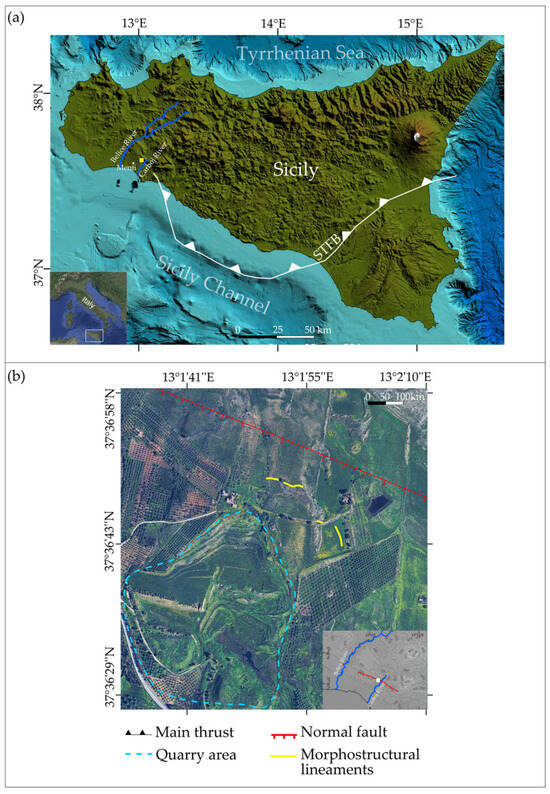
Figure 1.
(a) Location of the study area. STFB: Sicilian Fold-and-Thrust Belt [10]. The yellow square indicates the location of the area shown in the panel (b). The bathymetric data used in this map are derived from EMODnet (https://emodnet.ec.europa.eu/geoviewer/#, accessed on 29 April 2025), while the DEM for the onshore areas is obtained from the GMRT Map Tool (https://www.gmrt.org/GMRTMapTool/, accessed on 29 April 2025); (b) zoom of the study area. The location is indicated by the white square in the lower-right inset. The normal fault is derived from the ITHACA database (Italy Hazard from Capable faults) (https://sgi.isprambiente.it/ithaca/viewer/index.html, accessed on 29 April 2025).
Within the study area, morphostructural lineaments have been observed that are surface expressions that reflect underlying geological structures such as faults, fractures, or lithological boundaries. In particular, prominent lineaments trending WNW–ESE were identified, along with two minor lineaments northeast of the Bertolino quarry (yellow lines in Figure 1b): one parallel and one nearly perpendicular to the main trend. These lineaments were anthropogenically filled and subsequently reopened following a seismic swarm that occurred in the area in 2019.
Field investigations also revealed the presence of depressed elliptical areas in which mainly sandy deposits outcrop.
The aim of this paper is to investigate the role that seismicity has played in shaping the landscape, particularly focusing on the formation of fractures of potential tectonic origin or resulting from the mobilization of superficial deposits. To achieve this objective, a multidisciplinary approach was adopted.
We first conducted detailed field observations to identify and characterize open fractures, focusing on their geometry, orientation, and spatial distribution. To assess their temporal evolution, we analyzed a time series of high-resolution satellite imagery from Google Earth, which allowed us to detect changes in surface features potentially linked to fracture activity.
To further investigate the subsurface structure, we used the results from the MASW data interpretation to constrain the inversion of the HVSR curves, which allowed for the construction of thematic maps supporting preliminary structural interpretations.
To assess the liquefaction potential in the study area, we investigated the origin of the sediment samples collected from the elliptical and non-vegetated areas by analyzing their depositional environment. This approach, combined with HVSR results and Electrical Resistivity Tomography (ERT) investigations to identify the zones of underground fluid circulation associated with the fractures, helped clarify the processes involved.
2. Background
2.1. Geological and Geomorphological Settings
Western Sicily forms part of the external sector of the Sicilian Fold-and-Thrust Belt (SFTB) (Figure 1a), a south-verging contractional system that developed from the Neogene–Quaternary as a result of the ongoing convergence between the Nubian and Eurasian plates [11,12]. The region is structurally characterized by an imbricated stack of Mesozoic to Tertiary carbonate and clastic units, deformed during the Apennine–Maghrebian orogenic phase [11].
In the study area, the ITHACA database (Italy Hazard from Capable faults) (https://sgi.isprambiente.it/ithaca/viewer/index.html, accessed on 29 April 2025), which compiles active and capable fault systems across Italy, revealed the presence of a normal fault showing a WNW-ESE trend (red line in Figure 1b).
The research area is characterized by a hilly landscape with altitudes between 200 and 400 m. The landscape within the study area can be subdivided into two main sectors with distinct geomorphological and geological characteristics. The southern sector (red square in Figure 2a) includes the Bertolino quarry, where brown mudstone with levels of terrigenous sand of the Agrigento Formation (AGGa) are exposed [13]. The lithological composition of this formation results in weaker mechanical properties and a higher susceptibility to surface processes such as weathering and gullying (Figure 2b).
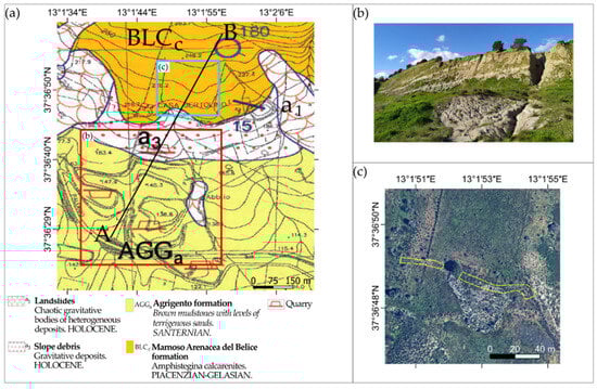
Figure 2.
(a) Excerpt from geological Sheet CARG 619 “Santa Margherita di Belice” [13]; (b) area characterized by erosion due to meteoric water flow; and (c) area showing the morphostructural lineaments trending WNW–ESE (yellow dashed lines).
In contrast, the northern sector of the study area (light blue square in Figure 2a,c) is characterized by more competent lithotypes belonging to the Marnoso Arenacea del Belice Formation, specifically to the BLCc member, composed of lithified biocalcarenites rich in Amphistegina [13]. In this sector, the erosive action of surface processes is less pronounced due to the lithological resistance. This geomorphological differentiation reflects not only lithological contrasts but also variations in structural control and surface dynamics.
A preliminary assessment of the geomorphological stability of the area was carried out through consultation of the PAI (Piano per l’Assetto Idrogeologico—Hydrogeological Management Plan) (https://www.sitr.regione.sicilia.it/pai/, accessed on 29 April 2025), particularly for hydrological basins 058 (Carboj River Basin) and 059 (area between the Carboj and Belice River basins). According to this source, the general morphological setting of the area appears to be in a condition of stable equilibrium.
2.2. Seismicity
Seismicity in western Sicily presents a complex framework that combines low-magnitude background activity with Mw values ranging between two and four (Figure 3), observed mainly in recent years due to the improvement of the seismic monitoring network, with stronger historical earthquakes, such as the 1968 Valle del Belice sequence (main event shown in Figure 3 with a red star). Available focal mechanism solutions, such as those reported by Scognamiglio et al. [14], indicate predominantly strike-slip mechanisms (Figure 3). However, the Belice Valley was generally considered a seismically inactive region, with no significant earthquakes documented in historical records or instrumental catalogs [12]. This perception was definitively overturned by the 1968, Mw 5.5, Belice seismic sequence, which represents the most intense seismic crisis recorded in western Sicily during historical times and which induced many authors [15,16,17,18] to extensively investigate the seismicity of this part of Sicily.
As reported by Lavecchia et al. [16], the sequence was characterized by eight main events, with moment magnitudes ranging from Mw 4.7 to 5.5, occurring between 14 and 25 January 1968, followed by hundreds of aftershocks that continued until June. Instrumental analyses by Monaco et al. [15] showed that the hypocenters of the main earthquakes were distributed along a north-dipping plane, with depths ranging from 36 km to 1 km, suggesting a vertically extensive seismogenic source. Other authors [19,20] described the seismic sequence as starting in January 1968 with several foreshocks, culminating in the mainshock (red star in Figure 3) on 15 January 1968, which reached a moment magnitude between Mw 5.5 and 5.8 and nucleated at a depth of about 10 km, causing widespread destruction in the area. The aftershocks continued in the following weeks, some exceeding Mw 5.0, amplifying the impact.
Field observations following the earthquake documented numerous coseismic effects, including landslides, ground ruptures, and fluid expulsion phenomena, particularly in lowland areas and along river valleys [12,20,21]. Despite extensive geophysical and geological investigations over the years, the seismotectonic framework of the Belice area remains not fully resolved. Various focal mechanism solutions for the 1968 events suggest a complex tectonic setting, with interpretations ranging from thrust faulting along WSW–ENE-oriented planes to right-lateral transpressional movements along NNW–SSE structures [22,23,24]. This variability highlights the persistent uncertainty regarding the precise identification and geometry of the seismogenic sources responsible for the 1968 sequence and, more broadly, for the seismicity of western Sicily.
A different scenario emerges in the following decades: according to Scarfi et al. [18], as well as to the CLASS [25] and ISIDe [26] seismic catalogs, instrumentally recorded seismicity has significantly increased since 2019. In particular, in July 2019, a seismic swarm was observed (red dashed line in Figure 3), with events occurring at depths between 6 km and 10 km and magnitudes ranging from Mw 2 to 2.8. It is observed that, in general, the hypocenters of these earthquakes progressively deepen from south to north.
These episodes, localized and of low magnitude, displayed the typical distribution of seismic swarms without a dominant mainshock, outlining the recent activity that is diffuse and of modest energy compared to the historical 1968 crisis.

Figure 3.
Distribution of earthquakes (circles in color scale according to depth). Seismic events (M ≥ 2) were extracted from the CLASS catalog [25] from 1981 and 2018 and from the ISIDe catalog [26] from 2005 to 2024. Events with uncertain hypocentral depth (quality class “E”) were excluded from the CLASS dataset. Available focal mechanisms are also shown [14,22,23,24]. The DEM is obtained from the GMRT Map Tool (https://www.gmrt.org/GMRTMapTool/, accessed on 29 April 2025).
3. Materials and Methods
3.1. Field Observation and Multi-Temporal Satellite Image Analysis
We conducted field surveys from 2019 to 2025. These field observations were essential for documenting surface features such as fractures, depressions, and ground displacements and for assessing their evolution over time.
To further extend the temporal coverage of our investigation, we analyzed the historical archive of satellite images available via Google Earth. This allowed us to identify and compare the morphological changes that occurred in the study area from 2014 to 2025.
3.2. Grain-Size and Morphoscopic Analyses
We collected 22 sediment samples from 15 different points across the study area (red squares in Figure 4). Specifically, we collected samples near morphostructural lineaments, within depressed elliptical areas, and from outcrops in the surrounding zones. At 7 of these sites, we collected samples both at surface and at depth to investigate vertical variations in sediment characteristics.
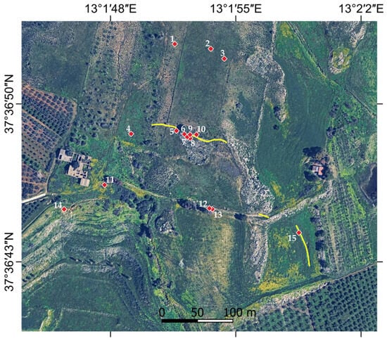
Figure 4.
Location of soil sampling sites (red squares) and morphostructural lineaments (yellow lines) within the study area.
To assess sediment provenance, depositional environment and transport mechanisms, we carried out both grain-size and morphoscopic analyses.
We performed the grain-size analysis in accordance with ASTM standards [27]. We initially pretreated the sediment samples with a solution of hydrogen peroxide and distilled water to remove organic material and soluble salts that could artificially link individual grains and change the grain-size distribution. We performed an initial wet sieving step using 63 µm mesh to separate the coarse (>63 µm) and fine (<63 µm) fractions. We dried the coarse fraction in an oven at 70 °C and then dry sieved it using a standard stack of sieves with mesh sizes of 2 mm, 1 mm, 0.5 mm, 250 µm, 125 µm, and 63 µm. The sieving phase was performed on a vibratory shaker for 5 min.
We allowed the fraction <63 μm to decant and then dried it in the oven for subsequent weighing.
We accurately weighed each grain-size fraction and calculated the weight percentage of each grain-size class to construct grain-size distribution curves.
Regarding morphoscopic analysis, we selected about 100 grains from the sediment samples. Some of the latter were excluded from this analysis because of their predominantly clay composition, which made them inappropriate for morphoscopic examination, since this method specifically targets quartz grains. We observed the selected grains under a Scanning Electron Microscope (SEM) and compared them with standard visual reference tables for sphericity [28], shape [29], and roundness [30]. This comparative approach allowed us to infer the probable transport mechanisms and depositional environments associated with each sediment sample.
3.3. HVSR and MASW: Ambient Noise and Surface Waves Methods
In this study, two passive seismic methods were employed to investigate subsurface stratigraphy and the potential seismic response: the Horizontal-to-Vertical Spectral Ratio (HVSR) method and the Multichannel Analysis of Surface Waves (MASW). These complementary approaches provide different but synergistic insights into the elastic properties and geometry of subsurface layers.
To investigate the distribution of subsurface fractures and their potential influence on surface deformation, we performed 41 HVSR measurements.
The HVSR method [31,32] is a widely used, non-invasive geophysical technique that analyzes ambient seismic vibrations produced by both natural sources (e.g., oceanic microseisms, wind) and anthropogenic activities. By computing the spectral ratio between the horizontal and vertical components of ground motion, the method allows for the identification of resonance frequencies, which are strongly influenced by impedance contrasts between overlying sediments and underlying bedrock. These frequencies are commonly interpreted to estimate sediment thicknesses and S-wave velocity profiles, often through empirical or semi-empirical relationships [33,34].
Furthermore, the spatial distribution of HVSR peak amplitudes and frequencies can yield insights into the geometry of subsurface geomorphological features, buried paleosurfaces, and tectonic structures [5,6,7].
The HVSR measurements that we performed were distributed around the identified morphostructural lineaments (yellow crosses in Figure 5). We recorded ambient seismic noise using a TROMINO® three-component digital seismic station. Each measurement consisted of an 18 min recording at a sampling frequency of 256 Hz.
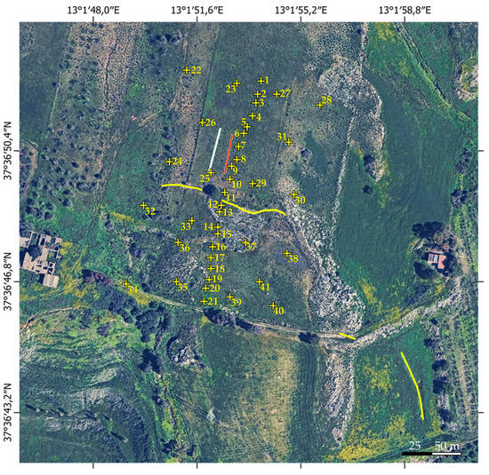
Figure 5.
Location of HVSR measurements (yellow crosses). The yellow, white, and red lines show the location of the morphostructural lineaments, ERT and MASW, respectively.
The quality and reliability of each HVSR curve were assessed according to the SESAME (Site Effects Assessment using Ambient Excitations) project guidelines [35], considering the following parameters: standard deviation stability, number of stable time windows, curve smoothness, and polarization anomalies. In Table A1, compliance with SESAME criteria is explicitly indicated.
We processed the acquired data using GRILLA software (version 7.0) [36] within a frequency range of 0.9–100 Hz, employing 20 s time windows and a 10% triangular smoothing function.
While the HVSR technique is effective in identifying impedance contrasts, it also has limitations. The method assumes a 1D layered medium, and the H/V peak may be ambiguous in complex stratigraphy or lateral heterogeneity. Additionally, the method does not provide absolute shear wave velocities unless combined with other geophysical data such as MASW [37,38,39].
To mitigate this ambiguity and improve the reliability of the velocity models, HVSR analysis was integrated with a MASW survey. The MASW method is based on the analysis of Rayleigh wave propagation. The dispersion curve (phase velocity vs. frequency) reflects the shear wave velocity distribution with depth. We acquired active surface wave data using a 12-channel geophone array (4.5 Hz vertical component), spaced at 2.5 m intervals, with a 5 m offset. The seismic source consisted of a 5 kg sledgehammer impacting a steel plate. Data has been processed using WinMASW® Academy software (version 7.0).
One of the known limitations of MASW is its sensitivity to the directionality of wave propagation and near-surface heterogeneities, which can distort dispersion curves. The lateral resolution is limited to approximately one-third of the array length, and higher frequencies are needed for shallow targets. Moreover, the inversion of dispersion curves is inherently non-unique, and model regularization plays a crucial role in constraining velocity profiles.
The 1D shear wave velocity (Vs) profiles obtained from MASW interpretation were used to constrain the inversion of the HVSR curves, specifically by providing reference velocity values for the shallowest layers (i.e., weathered zone and cover deposits). This integration ensured that the inverted HVSR models reflect realistic near-surface velocities and allowed for a more stable and physically consistent solution [40]. The resulting Vs models derived from HVSR inversion showed limited deviation from those obtained via MASW, while still achieving a satisfactory fit between observed and theoretical HVSR curves [41,42,43].
From the HVSR measurements, we generated thematic maps, including the fundamental frequency map, the associated H/V amplitude map, and a first layer thickness map.
To construct these maps, fundamental frequency (f0) and H/V amplitude values (A) were extracted from each HVSR curve. The spatial interpolation and visualization of these parameters were performed using Surfer software v.20, provided by Golden Software, LCC (Golden Software, LLC, Golden, CO, USA), applying a kriging algorithm on a 2 m × 2 m regular grid. The first-layer thickness (H) was estimated by assuming a horizontally layered model and applying the classical quarter-wavelength relation [43]:
where Vs is the shear wave velocity estimated from the MASW results, and f0 is the fundamental resonance frequency.
Finally, to further investigate the subsurface geometry, a distance–depth profile was constructed along the alignment of HVSR measurement points 1 to 21 (location in Figure 5), oriented perpendicular to the WNW–ESE-trending morphostructural lineaments. This profile was derived by plotting interface depths estimated from the f0 and Vs values.
Furthermore, we calculated the vulnerability index proposed by [8] to estimate the potential for ground damage based on the HVSR results. This index is defined as follows:
where Kg is the vulnerability index, A is the H/V amplitude value, and f0 is the fundamental frequency, which was computed at each HVSR measurement point.
Using these values, we generated a spatial distribution map of the vulnerability index. The map was created using 3D modeling Move Software, version 2022.1 (https://www.petex.com/pe-geology/move-suite/move/, accessed on 29 April 2025), applying a Delaunay triangulation interpolation method based on the HVSR data points.
3.4. Electrical Resistivity Tomography
In order to observe the possible presence of subsurface fluid circulation, we processed an Electrical Resistivity Tomography (ERT) along a profile parallel to the MASW survey (position indicated by the white line in Figure 5).
ERT is a reliable geophysical tool for providing information on the spatial distribution of subsurface resistivity, which can be correlated with lithological variations and fluid content [44,45].
The acquisition was made using a Wenner array configuration with 15 electrodes spaced at 2.5 m, resulting in a total profile length of 35 m. We processed and interpreted the dataset using the Res2DInv software version 4.07 (Geotomo Software) [46], applying the robust inversion algorithm, which is particularly effective in resolving the sharp resistivity contrasts associated with geological discontinuities or compact anthropogenic structures [47].
4. Results
4.1. Surface Evolutions
A preliminary assessment of surface dynamics was carried out through the analysis of time-series satellite imagery from Google Earth, covering the period from 2014 to 2024. In the northern sector of the quarry, morphostructural lineaments trending WNW–ESE were identified (Figure 1b, Figure 4 and Figure 5). These features appear to progressively elongate between 2014 (Figure 6b) and 2017 (Figure 6e). By 2018 (Figure 6f), these lineaments appear to have been filled anthropogenically. However, satellite images from 2020 (Figure 6g) clearly show that these features reopened, with a progressive eastward propagation from 2020 (Figure 6g) to 2024 (Figure 6i).
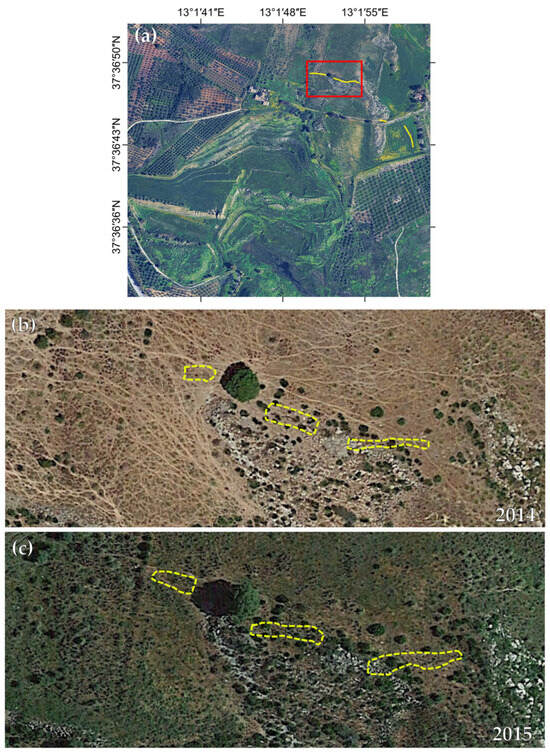
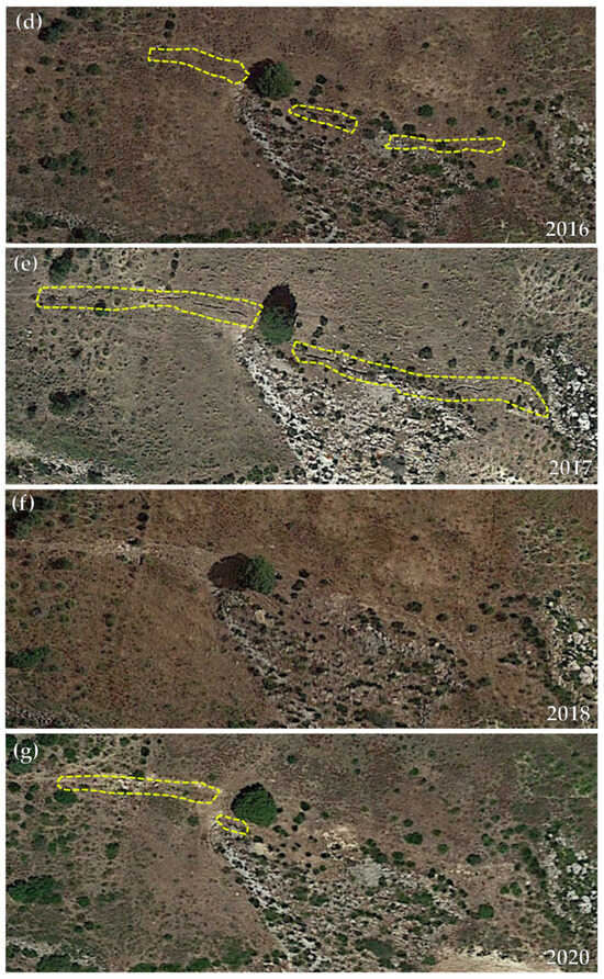
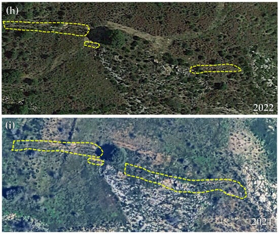
Figure 6.
Satellite imagery showing the temporal evolution of morphostructural lineaments northeast of the quarry. (a) The red rectangle shows the location of the detailed views in panels from (b) to (i). (b–i) Progressive development of WNW-ESE-oriented morphostructural lineaments. In the panel (d), the morphostructural lineaments are not visible, as they have been anthropogenically filled.
Additionally, in the northeastern sector of the quarry, another morphostructural lineament oriented approximately N–S was identified (dashed yellow lines in Figure 7c–i). This fracture shows a progressive spatial extension over the period analyzed, becoming increasingly evident and laterally continuous over time. Satellite imagery also revealed a progressive inclination of the tree row (dashed red lines in Figure 7b–i) from north to south over a 10-year period. In particular, the trees appear to tilt progressively southward, relative to the rural track above, probably in response to soil deformation processes.
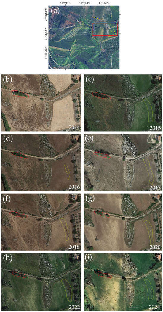
Figure 7.
Temporal evolution of satellite imagery from 2014 to 2024. (a) Map showing the location of the detailed views presented in panels (b) to (i). (b–i) Evolution of the NS trending morphostructural lineament (yellow dashed lines) and the progressive inclination of the tree row (red dashed lines) from north to south over time, as observed relative to the rural track above.
The same morphostructural lineaments observed in satellite imagery were also documented during field investigations beginning in 2019. These features presented as deep open fractures, in some cases exceeding 5 m in depth, and their lateral expansion was visibly progressing over time. Figure 8 shows this temporal evolution of the surface fractures, although field documentation was sometimes limited by dense vegetation, which restricted access to some locations. Furthermore, field observations conducted in 2025 led to the identification of new morphostructural lineaments that had not been previously detected, either through earlier in situ investigations or satellite imagery analysis (Figure 8i–k).
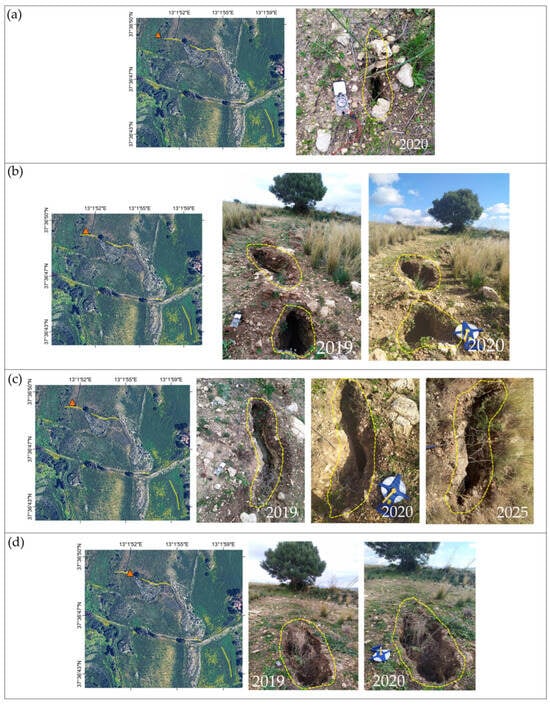
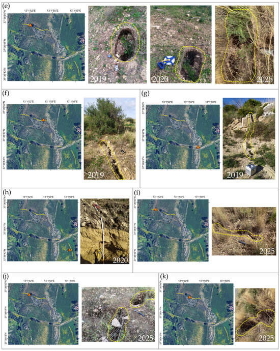
Figure 8.
Morphostructural lineaments (dashed yellow lines) observed in situ during field surveys from 2019 to 2025. In each panel, the morphostructural features are shown on the right and their location on the left (a–k).
In addition to the lineaments, field surveys identified three elliptical depressed areas that were not visible in satellite imagery (Figure 9). These structures were characterized by the absence of vegetation and were composed predominantly of sandy deposits. Each depression measured approximately 4 m × 3 m. These were first identified during field surveys conducted in 2020. However, in 2025, two of these features (Figure 9a,b) were not found, and their locations are, instead, characterized by the presence of open fractures (Figure 8k). In contrast, one of them is still evident in 2025 (Figure 9c).
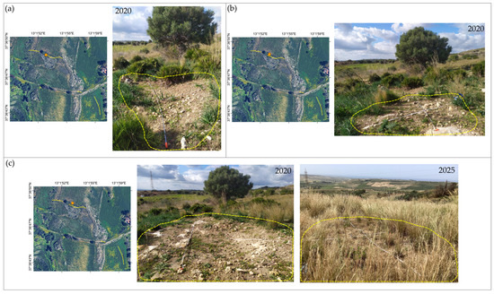
Figure 9.
Depressed elliptical areas (dashed yellow lines) without vegetation observed in the study area. Panels (a,b) show two such areas that are visible only in the 2020 field survey, and panel (c) shows one such area that is still observable in 2025.
4.2. Sedimentological Characterization
Through grain-size analysis, we determined the weight percentage of each granulometric class for all collected samples. These data were then used to construct grain-size distribution curves for each sample. The sampling locations are shown in Figure 4. Our results revealed that sandy fractions were predominant in most sediment samples, particularly those collected near the depressed elliptical areas and morphostructural lineaments. In contrast, finer grain-size distributions, with higher proportions of silt and clay, were observed in samples taken from distal areas. We assigned each sample the relative nomenclature reported in Table 1.

Table 1.
Name of sediment samples collected and their corresponding grain-size nomenclature. For sampling points where sediment samples were collected at both surface and depth, the terms “surface” and “depth” are used to distinguish them. Sampling locations are shown in Figure 4.
The morphoscopic analysis, conducted exclusively on the sandy samples since the method is applied to quartz grains, revealed that the quartz grains are predominantly equidimensional and exhibit similar degrees of sphericity and roundness [28,29,30]. The detailed morphoscopic characteristics of each sample are reported in Table 2.
Table 2.
Morphoscopic characteristics of quartz grains from the collected sediment samples. For each sample (sample names correspond to locations shown in Figure 4), the grain sphericity [29] and degree of roundness [30] are reported. The shape [28] is “equidimensional” for all samples.
A detailed morphoscopic analysis of all sandy samples allowed us to infer a likely marine origin for the quartz grains they contained. This interpretation is based on the presence of smoothed edges and small V-shaped percussion marks, both of which are characteristic features of marine depositional environments. Figure 10 presents a comparative example between a grain from one of the samples collected in the study area (Figure 10a) and a reference quartz grain of known marine origin [30] (Figure 10b).
Figure 10.
Comparison between (a) quartz grains from one of the sediment samples collected in the study area and (b) a reference grain representative of a marine depositional environment [30].
4.3. Geothematic Maps Used for Surface Deformation Analysis
The results of HVSR measurements are shown in Table 3. For clarity and transparency, all individual HVSR curves are presented in Figure A1, allowing for the visual inspection of resonance peaks. Additionally, Table A1 reports the SESAME compliance of each measurement point.
Table 3.
Results of HVSR measurements. The locations of measurement sites are shown in Figure 4.
The thematic maps of the fundamental frequencies, H/V amplitude ratios, and vulnerability indices (Kg), derived from these results, provide a summary of the subsurface vertical structure and degree of soil deformation at each measurement point.
A clear trend is evident from north to south across the study area, where a progressive decrease in the fundamental frequencies (Figure 11a) and in the H/V amplitude ratio (Figure 11b) is observed. This trend corresponds to the uppermost geological unit, the Marnoso Arenacea del Belice Formation, and indicates an increasing thickness of this layer. The transition is particularly abrupt near the morphostructural discontinuities trending WNW–ESE. This can be best observed in the first layer thickness map (Figure 11c) and in the distance–depth profile (Figure 11d).
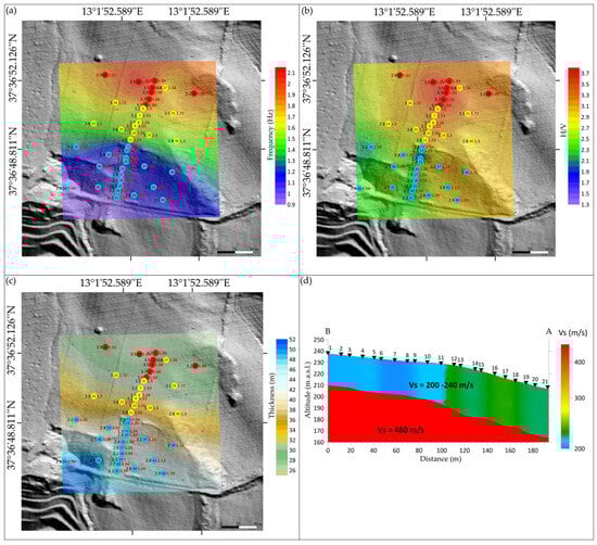
Figure 11.
(a) Fundamental frequency map; (b) H/V amplitude ratios; and (c) thickness map of the first layer. Circles represent HVSR measurement points (see Figure 5), colored according to fundamental frequency (f0): red = f0 > 1.8 Hz, yellow = 1.5–1.8 Hz, and light blue = f0 < 1.5 Hz. Numbers inside the circles indicate HVSR measurements, black numbers are H/V amplitude values, while red numbers indicate the corresponding fundamental frequency (see Table 3); (d) distance–depth profile (location in Figure 2a). Triangles mark the locations where the HVSR measurements were conducted.
Specifically, at HVSR measurement site 1, the Marnoso Arenacea del Belice Formation shows a thickness of approximately 26 m. Moving southward, a pronounced thickening of about 12 m is evident between HVSR sites 11 and 12, in correspondence with the WNW–ESE-trending fracture zone. This thickening results in a clean break in the slope that culminates in a maximum thickness of approximately 40 m at HVSR site 21.
This increase in interpreted depth is not attributable to the selection of higher Vs values in the equation, as the velocity variation along the profile is minor and was derived from HVSR inverse models constrained from MASW-derived ranges (Figure A2). Between HVSR sites 11 and 12, Figure 11d shows a slight increase in Vs of about 20 m/s, while the dominant feature is the marked reduction in f0, from 1.53 Hz at HVSR 11 to 0.94 Hz at HVSR 12. This decrease in resonance frequency is the main factor driving the significant increase in estimated thickness from Equation 1. Comparable f0 variations are also observed between other groups of HVSR sites highlighted in Figure 11. Therefore, the depth increase reflects genuine changes in resonance properties rather than artifacts of the velocity model.
The reliability of the HVSR-derived distance–depth profile, supported by the MASW-derived velocity models, shows compatible shear wave velocity distributions and confirms the presence of velocity contrasts at similar depths. The consistency between these independent methods enhances the robustness of the interpreted subsurface discontinuities.
Figure 12 shows the spatial distribution of the vulnerability index (Kg), calculated where the HVSR measurements are distributed (location in Figure 5). It ranges from 1.8 to 8.3. In the northern sector of the study area, Kg values are relatively uniform, generally ranging from 4.0 to 6.0. Closer to the morphostructural lineaments with a WNW-ESE trend, a marked increase is observed, with a maximum value of 8.3. south of this peak; Kg values decrease sharply, reaching their lowest values at the HVSR measurement point 14 (see location in Figure 5).
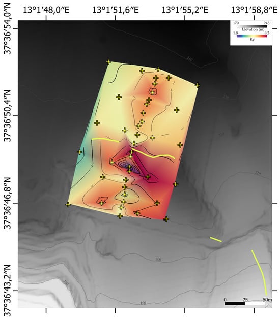
Figure 12.
Distribution map of the vulnerability index (Kg). Yellow lines and yellow crosses show morphostructural lineaments and the location of the HVSR measurements, respectively.
4.4. ERT
The inverted model of ERT (Figure 13c) presents the 2D resistivity model obtained from inversion, with an absolute error of about 1%, indicating a high-quality inversion result and a strong agreement between measured (Figure 13a) and calculated data (Figure 13b). ERT results reveal a resistivity distribution ranging from approximately 90 to over 800 Ω·m. Near-surface layers exhibit higher resistivity values, especially at the edges of the profile, potentially corresponding to dry or coarse-grained materials. The lateral variations indicate a significant heterogeneity in composition. The ERT profiles highlight a low-resistivity zone (<100 Ωm), approximately below a 3–5 m depth, interpreted as a saturated fine-grained layer. It is important to note that the survey was conducted in late September, following a dry summer period with no significant rainfall, as confirmed by local precipitation records. Therefore, the presence of this conductive layer suggests that saturation persists even during dry-season conditions, possibly due to low permeability and water retention in fine sediments. Nevertheless, since resistivity is sensitive to moisture content, we acknowledge that a detailed assessment of seasonal groundwater dynamics would re-quire dedicated piezometric monitoring, which is beyond the scope of this study.
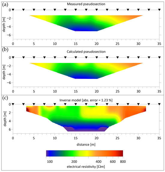
Figure 13.
Electrical Resistivity Tomography (ERT) results. (a) Measured apparent resistivity pseudosection; (b) calculated pseudosection from the inverted model; and (c) final 2D resistivity model. The color scale represents resistivity values in Ω·m. Triangles indicate electrode positions on the surface.
5. Discussion
The combined use of multi-temporal satellite imagery, field observations, and geophysical surveys enables a comprehensive interpretation of the surface deformations observed in the study area. Several lines of evidence converge to support the hypothesis of an ongoing and possibly reactivated mass movement process, which appears to be strongly controlled by structural and morphological processes.
Open fractures have been observed in the study area since 2014 (Figure 6). These features were filled anthropogenically in 2018, but their reopening is observed following a local seismic swarm in 2019, whose epicenters were located near the site (see dashed red line in Figure 3).
This temporal coincidence suggests that the earthquake could have acted as a trigger for the observed gravitational surface deformation, exploiting pre-existing weakness zones. Several studies have shown that low-magnitude earthquakes are capable of inducing slope failures, particularly when they occur in sequences that progressively weaken unstable slopes. Keefer [48], Rodríguez et al. [49], and Papadopoulos and Plessa [50] report cases where repeated small earthquakes contributed to triggering landslides, while Delgado et al. [51] documented the Montefrío event (southern Spain), where a very low-magnitude shock in October 1991 triggered a landslide. These observations are consistent with the dendrochronological analyses of Wistuba et al. [52], who demonstrated that recurrent low-magnitude earthquakes are more effective in destabilizing slopes than isolated ones, as exemplified by the 2007 Hałowiec landslide (Western Carpathians, Poland), which occurred after a sequence of nine earthquakes recorded between 2004 and 2006. In our study area, the landslide movement may have been further promoted by excavation activities in the quarry area immediately to the south. Such quarrying activity could have induced pre-existing instability before the earthquake, and this interpretation is consistent with Wistuba et al. [52], who emphasized that slopes already affected by stability problems require less seismic energy compared to the development of new landslides on previously stable slopes.
The area affected by the gravitational deformation is shown in Figure 14a.
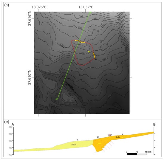
Figure 14.
(a) Area affected by gravitational deformation (dashed red line). The yellow lines and green line represent the morphostructural lineaments and the location of the geological section trace shown in (b), respectively; (b) geological cross-section (location in Figure 2a and Figure 14a). The black triangles labeled “1”, “11”, “12”, and “21” indicate the position of HVSR measurements, which correspond to those shown in Figure 5. The red arrow marks the location of morphostructural lineaments along the cross-section.
Field observations confirm that these fractures are not shallow: in some cases, their depth exceeds 5 m. In addition, a morphostructural lineament with a N-S trend was identified in the southeastern sector of the study area. To the west of this lineament, the trees appear to be increasingly sloping southward over time, as revealed by multi-temporal satellite analysis (dashed red lines in Figure 7). Based on this evidence, we hypothesize the presence of a slow-moving landslide affecting the area between the morphostructural lineaments, with a WNW-ESE trend to the north and the quarry area to the south and limited to the east by the NS-trending lineament.
The WNW-ESE trending fracture system may reflect extensional stress generated by the movement of the landslide body. Instability is likely facilitated by zones of weakness, such as pre-existing tectonic and geomorphological lineaments. For instance, a gully is clearly visible in the satellite imagery (dashed yellow line in Figure 7) in the sector that bounds the landslide to the east, and a fault mapped in the ITHACA database (https://sgi.isprambiente.it/ithaca/viewer/index.html, accessed on 29 April 2025) shows the same WNW–ESE orientation of the morphostructural features observed in the field. This spatial and structural agreement suggests a genetic link between seismic activity, landslide processes, and lineament development.
A detailed comparison was carried out among the depth estimates obtained through the HVSR method (using the quarter-wavelength relation), the shear wave velocity models from MASW, and the resistivity section from the ERT survey. Although the methods differ in physical principle, resolution, and investigation depth, they converge toward a coherent interpretation of the shallow subsurface structure.
The MASW data revealed a layered velocity model, including a shallow velocity inversion in the uppermost meter where a slightly stiffer layer (Vs > 300 m/s), likely representing a weathered or compacted crust, overlays a thinner, lower-velocity horizon (Vs ≈ 250 m/s), possibly related to looser or moisture-rich material. This inversion, while identifiable in the MASW model, was not incorporated into the inversion of the HVSR curves, as its limited thickness and weak impedance contrast fall below the resolution capabilities of the HVSR technique. Instead, average Vs values from the MASW results for the upper 5–10 m were used to constrain the HVSR inversion, ensuring consistency with the main impedance contrast and preserving a good match between observed and theoretical HVSR curves.
The ERT survey, with a maximum investigation depth of approximately 6–7 m, highlights a low-resistivity zone (<100 Ωm) extending from approximately 3–4 m down to the maximum depth investigated. This conductive horizon is consistent with the low-velocity zone identified in the MASW profile, supporting the presence of moisture-rich materials. This conductive layer is interpreted as a saturated, fine-grained unit, possibly corresponding to the lower-velocity zone observed in the MASW model. However, due to its limited penetration, the ERT profile does not resolve the deeper contrast identified by seismic methods between the soft sediments and the underlying stiffer substratum.
Overall, the integration of the three datasets supports a two-layer subsurface model composed of an upper, soft, and saturated cover, variable in thickness and electrical properties, and a more consolidated and mechanically stiffer unit at greater depth, imaged clearly by HVSR.
Minor discrepancies in estimated depths are expected, given the different physical sensitivities of the methods: HVSR and MASW respond to seismic velocity contrasts, while ERT reflects variations in resistivity influenced by lithology and water content. Despite these differences, the results are complementary and coherent, reinforcing the reliability of the interpreted subsurface structure.
Additional field observations revealed elliptical, vegetation-free depressions, which were confirmed as deposits containing sand based on the grain-size analysis (samples 7, 8, and 10 in Table 3).
Although recent seismicity recorded in the study area (Figure 3) has not reached intensities considered sufficient to trigger liquefaction processes [53,54], the geometry and sedimentological characteristics of these depressions strongly resemble those associated with liquefaction-induced features [4].
ERT results (Figure 13) indicate a low-resistivity zone at approximately 3–4 m depth, which may suggest the presence of subsurface water. This is probably related to the infiltration of meteoric water detained within the sandy lenticles that serve as temporary aquifers.
These fluids could play a key role in reducing effective stress and triggering liquefaction processes. However, an alternative explanation is that these fluids derive from rainfall infiltration and are retained in shallow, sandy lenses. Morphoscopic analyses of the sands extracted from the depressions reveal a marine depositional origin, ruling out recent continental inputs. This strongly supports the hypothesis that the sand may have migrated from the subsurface, possibly due to upward movement associated with liquefaction.
To test the liquefaction process hypothesis, we calculated the soil vulnerability index (Kg) [8]. According to [4], higher values of Kg correspond to a higher liquefaction potential. The resulting vulnerability index map (Figure 12) shows a significant peak in Kg values in proximity to the WNW-ESE morphostructural lineament, supporting the possibility of seismic-induced liquefaction. The rising of the sand could therefore have been caused by seismic shaking and/or by differences in density of the material under compressive stress. Furthermore, we hypothesize that these sandy materials may have used pre-existing morphostructural lineaments as preferential pathways for upward migration. Supporting this, field evidence shows that, over time, open fractures (Figure 8k) have developed in the exact location where two sandy elliptical depressions were previously observed (Figure 9a,b), and deposits containing sand were also identified in correspondence with the fractures (see Table 3). This suggests a mechanical link between liquefaction and fracturing.
To investigate how these structures develop in depth, we analyzed stratigraphic variations derived from HVSR profiles. Between HVSR measurement points 11 and 12 (location in Figure 5), we observed a progressive increase in the thickness of the Marnoso Arenacea del Belice Formation, coinciding with the WNW–ESE-trending lineaments. This discontinuity is also associated with a pronounced slope break in the topography (Figure 11d). We hypothesized two causes for this result: (i) a buried morphostructural feature inherited from a paleo-landscape and/or (ii) a subsurface discontinuity not exposed to the surface. An interpretative sketch of the possible subsurface configuration is shown in Figure 14b.
These structures produce differential seismic responses in the study area, as confirmed by the frequency map (Figure 11a), where there is a clear contrast in the soil behavior between the northern and southern sectors of the WNW-ESE lineaments.
6. Conclusions
This study presents a multidisciplinary investigation into the surface deformations and subsurface structures in the area east of Menfi, southwestern Sicily.
The main findings of this research can be summarized as follows:
- (i)
- The reopening of anthropogenically filled fractures following the 2019 seismic swarm suggests that even low-intensity seismicity can trigger or reactivate near-surface gravitational deformations along pre-existing structural weaknesses.
- (ii)
- Field observations and multi-temporal Google Earth imagery reveal the presence of a slow-moving landslide bounded by morphostructural lineaments trending WNW–ESE and N–S. The landslide’s development appears structurally controlled and possibly influenced by nearby quarry excavations.
- (iii)
- The integration of geophysical data (HVSR, MASW, and ERT) allowed for the characterization of a two-layer subsurface model, consisting of a shallow, saturated, mechanically soft cover overlying a more consolidated substratum. This model supports the interpretation of zones prone to liquefaction and fluid circulation linked to surface fractures.
- (iv)
- Grain-size and morphoscopic analyses of sandy deposits in elliptical depressions strongly indicate a marine origin and support the hypothesis of the upward migration of sediment through preferential pathways created by structural lineaments, consistent with liquefaction processes induced or enhanced by seismic shaking.
- (v)
- The calculated seismic vulnerability index (Kg) highlights the areas susceptible to liquefaction, spatially correlating with observed fractures
Overall, the combined geological and geophysical approach, together with field observation and satellite imagery analysis, highlights the complex relationship between seismicity, surface deformation, and liquefaction potential. These findings improve the understanding of earthquake-related secondary effects and contribute to assessing geological hazards in the region.
While geophysical data provide valuable constraints on the mechanical and hydrological structure of the subsurface, we recognize the inherent limitations of extrapolating localized measurements (such as MASW-derived Vs) across broader areas, as well as the time-dependent nature of subsurface saturation inferred from ERT. Future investigations should include piezometric monitoring and multi-seasonal surveys to fully capture the spatial and temporal variability relevant to slope stability and liquefaction assessment.
Furthermore, based on the evidence provided by this research, we suggest reviewing the current classification of the study area considered as stable in the Italian Hydrogeological Management Plan.
Author Contributions
Conceptualization, S.B., R.M., M.G.M. and A.S.; methodology, S.B. and R.M.; validation, A.C., M.G.M. and A.S.; formal analysis, S.B. and R.M.; investigation, S.B., M.G.M., A.C. and A.S.; resources, M.G.M. and A.S.; writing—original draft preparation, S.B.; writing—review and editing, S.B., R.M., A.C., M.G.M. and A.S.; visualization, S.B. and R.M.; supervision, A.S. All authors have read and agreed to the published version of the manuscript.
Funding
This research received no external funding.
Institutional Review Board Statement
Non applicable.
Informed Consent Statement
Not applicable.
Data Availability Statement
The data used in this paper can be provided by the authors under reasonable request.
Acknowledgments
The authors would like to thank the GEOCiMA Laboratory (Palermo) for providing the raw MASW and ERT acquisition data, which were essential for the geophysical analyses conducted in this study.
Conflicts of Interest
The authors declare no conflicts of interest.
Appendix A

Figure A1.
Individual HVSR curves acquired in the study area. The curves are color-coded to emphasize their spatial position relative to the WNW–ESE-oriented fracture: red curves correspond to HVSR measurements collected north of the fracture (see locations of HVSR points 1–11 and 22–31 in Figure 5), while blue curves represent those collected south of the fracture (see HVSR points 12–21 and 32–41 in Figure 5).
Table A1.
Summary of the SESAME criteria compliance for each of the 41 HVSR measurement points.
Table A1.
Summary of the SESAME criteria compliance for each of the 41 HVSR measurement points.
| ID | Criteria for a Reliable H/V Curve | Criteria for a Clear H/V Peak | |||||||
|---|---|---|---|---|---|---|---|---|---|
| f0 > 10/Lw | nc(f0) > 200 | σA(f) < 2 for 0.5f0 < f < 2f0 If f0 > 0.5 Hz σA(f) < 3 for 0.5f0 < f < 2f0 If f0 < 0.5 Hz | Exists f − in [f0/4, f0] | AH/V (f −) < A0/2 | Exists f + in [f0, 4f0] | AH/V (f +) < A0/2 | A0 > 2 | fpeak[AH/V(f) ± σA(f)] = f0 ± 5% | σf < ε(f0) | σA(f0) < θ(f0) | |
| 1 | OK | OK | OK | OK | OK | OK | OK | OK | OK |
| 2 | OK | OK | OK | OK | OK | OK | NO | NO | OK |
| 3 | OK | OK | OK | OK | OK | OK | NO | OK | OK |
| 4 | OK | OK | OK | OK | OK | OK | NO | NO | OK |
| 5 | OK | OK | OK | OK | OK | OK | NO | NO | OK |
| 6 | OK | OK | OK | NO | OK | OK | NO | NO | OK |
| 7 | OK | OK | OK | NO | OK | OK | NO | NO | OK |
| 8 | OK | OK | OK | NO | OK | OK | NO | OK | OK |
| 9 | OK | OK | OK | OK | OK | OK | NO | NO | OK |
| 10 | OK | OK | OK | NO | OK | OK | NO | OK | OK |
| 11 | OK | OK | OK | NO | OK | OK | NO | NO | OK |
| 12 | OK | OK | OK | NO | OK | OK | NO | NO | OK |
| 13 | OK | OK | OK | NO | OK | OK | NO | NO | OK |
| 14 | OK | OK | OK | NO | OK | OK | NO | NO | OK |
| 15 | OK | OK | OK | NO | OK | OK | NO | NO | OK |
| 16 | OK | OK | OK | NO | OK | OK | NO | NO | OK |
| 17 | OK | OK | OK | NO | OK | OK | NO | NO | OK |
| 18 | OK | OK | OK | NO | OK | OK | NO | NO | OK |
| 19 | OK | OK | OK | NO | OK | OK | NO | OK | OK |
| 20 | OK | OK | OK | NO | OK | OK | NO | NO | OK |
| 21 | OK | OK | OK | NO | OK | OK | NO | OK | OK |
| 22 | OK | OK | OK | OK | OK | OK | OK | OK | OK |
| 23 | OK | OK | OK | OK | OK | OK | NO | NO | OK |
| 24 | OK | OK | OK | OK | OK | OK | NO | NO | OK |
| 25 | OK | OK | OK | NO | OK | OK | OK | OK | OK |
| 26 | OK | OK | OK | OK | OK | OK | OK | OK | OK |
| 27 | OK | OK | OK | NO | OK | OK | NO | NO | OK |
| 28 | OK | OK | OK | OK | OK | OK | NO | NO | OK |
| 29 | OK | OK | OK | NO | OK | OK | NO | NO | OK |
| 30 | OK | OK | OK | OK | OK | OK | NO | NO | OK |
| 31 | OK | OK | OK | OK | OK | OK | NO | OK | OK |
| 32 | OK | OK | OK | NO | OK | OK | NO | NO | OK |
| 33 | OK | OK | OK | NO | OK | OK | NO | NO | OK |
| 34 | OK | OK | OK | NO | OK | OK | OK | OK | OK |
| 35 | OK | OK | OK | NO | OK | OK | NO | NO | OK |
| 36 | OK | OK | OK | NO | OK | OK | NO | NO | OK |
| 37 | OK | OK | OK | NO | OK | OK | NO | NO | OK |
| 38 | OK | OK | OK | OK | OK | OK | OK | OK | OK |
| 39 | OK | OK | OK | OK | OK | OK | NO | NO | OK |
| 40 | OK | OK | OK | OK | OK | OK | NO | NO | OK |
| 41 | OK | OK | OK | NO | OK | OK | NO | NO | OK |

Figure A2.
MASW dispersion curve (phase velocity vs. frequency) (a) and corresponding 1D shear wave velocity profile (b) obtained from inversion.
References
- McCalpin, J. Paleoseismology, 2nd ed.; Academic Press: San Diego, CA, USA; London, UK, 2009; Volume 629. [Google Scholar]
- De Martini, P.M.; Cinti, F.R.; Cucci, L.; Smedile, A.; Pinzi, S.; Brunori, C.A.; Molisso, F. Sand volcanoes induced by the April 6th 2009 Mw 6.3 L’Aquila earthquake: A case study from the Fossa area. Ital. J. Geosci. 2012, 131, 410–422. [Google Scholar] [CrossRef]
- Tallini, M.; Maceroni, D.; Falcucci, E.; Galadini, F.; Gori, S.; Guerriero, V.; Spadi, M.; Moro, M.; Saroli, M. Multi-methodological approach for assessing surface faulting and paleoliquefaction history in central Italy: Applicative implications for seismic microzonation studies in the Quaternary L’Aquila basin. Front. Earth Sci. 2025, 13, 1523730. [Google Scholar] [CrossRef]
- Akkaya, I. Availability of Seismic Vulnerability Index (Kg) in the Assessment of Building Damage in Van, Eastern Turkey. Earthq. Eng. Eng. Vib. 2020, 19, 189–204. [Google Scholar] [CrossRef]
- Grippa, A.; Bianca, M.; Tropeano, M.; Cilumbriello, A.; Gallipoli, M.R.; Mucciarelli, M.; Sabato, L. Use of the HVSR method to detect buried paleomorphologies (filled incised-valleys) below a coastal plain: The case of the Metaponto plain (Basilicata, southern Italy). Boll. Geofis. Teor. Appl. 2011, 52, 225–240. [Google Scholar]
- Tarabusi, G.; Caputo, R. The use of HVSR measurements for investigating buried tectonic structures: The Mirandola anticline, Northern Italy, as a case study. Int. J. Earth Sci. 2017, 106, 341–353. [Google Scholar] [CrossRef]
- Mele, M.; Bersezio, R.; Bini, A.; Bruno, M.; Giudici, M.; Tantardini, D. Subsurface profiling of buried valleys in central alps (northern Italy) using HVSR single-station passive seismic. J. Appl. Geophys. 2021, 193, 104407. [Google Scholar] [CrossRef]
- Nakamura, Y. Seismic Vulnerability Indices for Ground and Structures Using Microtremor. In Proceedings of the World Congress on Railway Research, Florence, Italy, 16–19 November 1997; pp. 1–7. [Google Scholar]
- Alonso-Pandavenes, O.; Torrijo, F.J.; Torres, G. Analysis of the Liquefaction Potential at the Base of the San Marcos Dam (Cayambe, Ecuador)—A Validation in the Use of the Horizontal-to-Vertical Spectral Ratio. Geosciences 2024, 14, 306. [Google Scholar] [CrossRef]
- Sulli, A.; Morticelli, M.G.; Agate, M.; Zizzo, E. Active north-vergent thrusting in the Northern Sicily continental margin in the frame of the quaternary evolution of the Sicilian collisional system. Tectonophysics 2021, 802, 228717. [Google Scholar] [CrossRef]
- Catalano, R.; Franchino, A.; Merlini, S.; Sulli, A. Central western Sicily structural setting interpreted from seismic reflection profiles. Mem. Soc. Geol. It 2000, 55, 5–16. [Google Scholar]
- Barreca, G.; Bruno, V.; Cocorullo, C.; Cultrera, F.; Ferranti, L.; Guglielmino, F.; Guzzetta, L.; Mattia, M.; Monaco, C.; Pepe, F. Geodetic and geological evidence of active tectonics in south-western Sicily (Italy). J. Geodyn. 2014, 82, 138–149. [Google Scholar] [CrossRef]
- Di Stefano, P.; Renda, P.; Zarcone, G.; Nigro, F.; Cacciatore, M.S.; Di Stefano, E.; Sprovieri, R.; Bonomo, S.; Monteleone, S.; Sabatino, M. Note Illustrative della Carta Geologica d’Italia Allascala 1:50.000—Foglio 619 S. Margherita Belice; ISPRA, Servizio Geologico d’Italia, Regione Siciliana—Assessorato Territorio e Ambiente, SystemCart: Rome, Italy, 2013; pp. 1–178.
- Scognamiglio, L.; Tinti, E.; Quintiliani, M. Time Domain Tensor (TDMT) [Data Set]; Istituto Nazionale di Geofisica e Vulcanologia (INGV): Rome, Italy, 2006. [CrossRef]
- Monaco, C.; Mazzoli, S.; Tortorici, L. Active thrust tectonics in western Sicily (southern Italy): The 1968 Belice earthquake sequence. Terra Nova 1996, 8, 372–381. [Google Scholar] [CrossRef]
- Lavecchia, G.; Ferrarini, F.; de Nardis, R.; Visini, F.; Barbano, M.S. Active thrusting as a possible seismogenic source in Sicily (Southern Italy): Some insights from integrated structural–kinematic and seismological data. Tectonophysics 2007, 445, 145–167. [Google Scholar] [CrossRef]
- Azzaro, R.; Barbano, M.S.; Tertulliani, A.; Pirrotta, C. A reappraisal of the 1968 Valle del Belìce seismic sequence (western Sicily): A case study of intensity assessment with cumulated damage effects. Ann. Geophys. 2020, 63, SE105. [Google Scholar] [CrossRef]
- Scarfì, L.; Barberi, G.; Barreca, G.; Musumeci, C.; Tusa, G. Insights into Western Sicily’s seismotectonics from recent seismicity and 1968 Belice mainshock ground motion simulations. Nat. Hazards 2025, 121, 5757–5780. [Google Scholar] [CrossRef]
- Rovida, A.; Locati, M.; Camassi, R.; Lolli, B.; Gasperini, P. The Italian earthquake catalogue CPTI15. Bull. Earthq. Eng. 2020, 18, 2953–2984. [Google Scholar] [CrossRef]
- Rovida, A.; Locati, M.; Camassi, R.; Lolli, B.; Gasperini, P.; Antonucci, A. Catalogo Parametrico dei Terremoti Italiani (CPTI15), Versione 4.0 [Data Set]; Istituto Nazionale di Geofisica e Vulcanologia (INGV): Rome, Italy, 2022. [CrossRef]
- Bosi, C.; Cavallo, R.; Francaviglia, V. Aspetti geologici e geologico-tecnici del terremoto della Valle del Belice del 1968. Mem. Soc. Geol. Ital. 1973, 12, 81–130. [Google Scholar]
- McKenzie, D. Active tectonics of the Mediterranean Region. Geophys. J. Int. 1972, 30, 109–185. [Google Scholar] [CrossRef]
- Gasparini, c.; Iannaccone, G.; Scarpa, R. Fault-plane solutions and seismicity of the Italian peninsula. Tectonophysics 1985, 117, 59–78. [Google Scholar] [CrossRef]
- Anderson, H.; Jackson, J. Active tectonics of the Adriatic Region. Geophys. J. Int. 1987, 91, 937–983. [Google Scholar] [CrossRef]
- Latorre, D.; Di Stefano, R.; Castello, B.; Michele, M.; Chiaraluce, L. Catalogo delle Localizzazioni ASSolute (CLASS), (Version 1); Istituto Nazionale di Geofisica e Vulcanologia (INGV): Rome, Italy, 2022. [CrossRef]
- ISIDe Working Group. ISIDe, Italian Seismological Instrumental and Parametric Database, Version 1.0; Istituto Nazionale di Geofisica e Vulcanologia (INGV): Rome, Italy, 2016. [CrossRef]
- ASTM. Test Designation D422. Standard Method for Particle Size Analysis of Soils; ASTM: Philadelphia, PA, USA, 1972. [Google Scholar]
- Zingg, T. Beitrag zur Shotteranalyse. Schweiz. Min. u. Pet. Mitt. 1935, 15, 39–140. [Google Scholar]
- Rittenhouse, G. Measuring intercept sphericity of sand grains. Am. J. Sci. 1943, 241, 109. [Google Scholar] [CrossRef]
- Powers, M.C. A new roundness scale for sedimentary particles. J. Sediment. Res. 1953, 23, 117–119. [Google Scholar] [CrossRef]
- Nakamura, Y. A method for dynamic characteristics estimation of subsurface using microtremor on the ground surface. Railway Technical Research Institute. Q. Rep. 1989, 30, 25–33. [Google Scholar]
- Nakamura, Y. What is the Nakamura method? Seismol. Res. Lett. 2019, 90, 1437–1443. [Google Scholar] [CrossRef]
- Ibs-von Seht, M.; Wohlenberg, J. Microtremor measurements used to map thickness of soft sediments. Bull. Seism. Soc. Am. 1999, 89, 250–259. [Google Scholar] [CrossRef]
- Delgado, J.; Casado, C.L.; Estevez, A.; Giner, J.; Cuenca, A.; Molina, S. Mapping soft soils in the Segura river valley (SE Spain): A case study of microtremors as an exploration tool. J. Appl. Geophys. 2000, 45, 19–32. [Google Scholar] [CrossRef]
- Havenith, H.B. Guidelines for the Implementation of the H/V Spectral Ratio Technique on Ambient Vibrations Measurements, Processing and Interpretation. 2004. Available online: http://sesame.geopsy.org/Papers/HV_User_Guidelines.pdf (accessed on 29 April 2025).
- Micromed. Dati Tecnici Tromino e Download Pacchetto Software Grilla. 2011. Available online: http://www.tromino.it (accessed on 29 April 2025).
- Fäh, D.; Kind, F.; Giardini, D. A theoretical investigation of average H/V ratios. Geophys. J. Int. 2001, 145, 535–549. [Google Scholar] [CrossRef]
- Canzoneri, A.; Capizzi, P.; Martorana, R.; Albano, L.; Bonfardeci, A.; Costa, N.; Favara, R. Geophysical Constraints to Reconstructing the Geometry of a Shallow Groundwater Body in Caronia (Sicily). Water 2023, 15, 3206. [Google Scholar] [CrossRef]
- Canzoneri, A.; Martorana, R.; Agate, M.; Gasparo Morticelli, M.; Capizzi, P.; Carollo, A.; Sulli, A. Reconstruction of a 3D Bedrock Model in an Urban Area Using Well Stratigraphy and Geophysical Data: A Case Study of the City of Palermo. Geosciences 2025, 15, 174. [Google Scholar] [CrossRef]
- Park, C.B.; Miller, R.D.; Xia, J. Multichannel analysis of surface waves. Geophysics 1999, 64, 800–808. [Google Scholar] [CrossRef]
- Zor, E.; Özalaybey, S.; Karaaslan, A.; Tapirdamaz, M.C.; Özalaybey, S.Ç.; Tarancioglu, A.; Erkan, B. Shear wave velocity structure of the Izmit Bay area (Turkey) estimated from active-passive array surface wave and single-station microtremor methods. Geophys. J. Int. 2010, 182, 1603–1618. [Google Scholar] [CrossRef]
- Capizzi, P.; Martorana, R. Integration of constrained electrical and seismic tomographies to study the landslide affecting the Cathedral of Agrigento. J. Geophys. Eng. 2014, 11, 045009. [Google Scholar] [CrossRef]
- Panzera, F.; Sicali, S.; Lombardo, G.; Imposa, S.; Gresta, S.; D’Amico, S. A microtremor survey to define the subsoil structure in a mud volcanoes area: The case study of Salinelle (Mt. Etna, Italy). Environ. Earth Sci. 2016, 75, 1140. [Google Scholar] [CrossRef]
- Reynolds, J.M. An Introduction to Applied and Environmental Geophysics, 2nd ed.; Wiley-Blackwell: Hoboken, NJ, USA, 2011. [Google Scholar]
- Binley, A.; Kemna, A. DC resistivity and induced polarization methods. In Hydrogeophysics; Springer: Dordrecht, The Netherlands, 2005; pp. 129–156. [Google Scholar]
- Loke, M.H. Tutorial: 2-D and 3-D Electrical Imaging Surveys. 2013. Available online: www.geotomosoft.com (accessed on 29 April 2025).
- Loke, M.H.; Barker, R.D. Rapid least-squares inversion of apparent resistivity pseudosections using a quasi-Newton method. Geophys. Prospect. 1996, 44, 131–152. [Google Scholar] [CrossRef]
- Keefer, D.K. Landslides caused by earthquakes. Geol. Soc. Am. Bull. 1994, 95, 406–421. [Google Scholar] [CrossRef]
- Rodríguez, C.E.; Bommer, J.J.; Chandler, R.J. Earthquake-induced landslides: 1980–1997. Soil Dyn. Earthq. Eng. 1999, 18, 325–346. [Google Scholar] [CrossRef]
- Papadopoulos, G.A.; Plessa, A. Magnitude-distance relations for earthquake–induced landslides in Greece. Eng. Geol. 2000, 58, 377–386. [Google Scholar] [CrossRef]
- Delgado, J.; Garrido, J.; López-Casado, C.; Martino, S.; Peláez, J.A. On far field occurrence of seismically induced landslides. Eng. Geol. 2011, 123, 204–213. [Google Scholar] [CrossRef]
- Wistuba, M.; Malik, I.; Krzemień, K.; Gorczyca, E.; Sobucki, M.; Wrońska-Wałach, D.; Gawior, D. Can low-magnitude earthquakes act as a triggering factor for landslide activity? Examples from the Western Carpathian Mts, Poland. CATENA 2018, 171, 359–375. [Google Scholar] [CrossRef]
- Galli, P. New empirical relationships between magnitude and distance for liquefaction. Tectonophysics 2000, 324, 169–187. [Google Scholar] [CrossRef]
- Papathanassiou, G.; Pavlides, S.; Ganas, A. The 2003 Lefkada earthquake: Field observations and preliminary microzonation map based on liquefaction potential index for the town of Lefkada. Eng. Geol. 2005, 82, 12–31. [Google Scholar] [CrossRef]
Disclaimer/Publisher’s Note: The statements, opinions and data contained in all publications are solely those of the individual author(s) and contributor(s) and not of MDPI and/or the editor(s). MDPI and/or the editor(s) disclaim responsibility for any injury to people or property resulting from any ideas, methods, instructions or products referred to in the content. |
© 2025 by the authors. Licensee MDPI, Basel, Switzerland. This article is an open access article distributed under the terms and conditions of the Creative Commons Attribution (CC BY) license (https://creativecommons.org/licenses/by/4.0/).