Secondary Education Students’ Misconceptions on Principles of Geology: Minerals and Rocks

Abstract

The purpose of this research is to investigate the misconceptions related to geological concepts among Secondary Education students in the region of Achaia, Greece. The study focuses on both Lower Secondary Education (Gymnasium, grades 7–9) and Upper Secondary Education, including General and Vocational Education (grades 10–12). Previous research has shown that students entering Lower Secondary Education or High School often possess several misconceptions about geological concepts. These misconceptions result in a fragmented or incorrect understanding, which may arise from intuitive perceptions of how the natural world evolves that are incorrect, or from stereotypes and assumptions acquired from the family environment or inadequacies in the school curriculum. Despite teachers’ efforts to clarify these concepts, a significant percentage of students continue to hold misconceptions, mainly related to minerals and rocks. A total of 1065 secondary students completed an online closed-ended questionnaire that was designed and validated based on previous research findings to highlight their misconceptions. This study results showed a clear differentiation between students from urban and rural areas, while demographic characteristics (such as gender, age, parents’ occupation, and parents’ marital status) did not appear to play a significant role. In addition, the responses to specific sets of questions varied depending on the student’s grade level. Identifying students’ misconceptions can support the development of appropriate educational tools and/or inform targeted interventions that aim to clarify these concepts and correct any incorrect assumptions.

1. Introduction

Research in the field of cognitive development has shown that children from an early age begin to construct intuitive frameworks or “naïve theories” to make sense of the world around them, explain everyday phenomena, and make predictions [1,2,3,4,5,6]. These theories are constructed based on everyday experiences, informal interactions, and the influence of lay culture. Although they serve as useful tools for interpreting natural phenomena, they often lead to the development of misconceptions. These misconceptions are not random errors, but coherent and internally consistent ideas that function much like scientific theories, yet lack empirical grounding.

Given the fact that naïve theories are based on everyday experience, they are notably resistant to change, even in the face of formal instruction. Correcting them requires more than simply replacing incorrect ideas with the scientifically accepted ones. Rather, it involves conceptual changes across multiple dimensions: ontological (how entities are categorized), epistemological (how knowledge is justified), and representational (how concepts are mentally visualized and expressed). These conceptual changes do not happen overnight but need a lot of time. During this process, new misconceptions may appear, which have the form of fragmented or synthetic conceptions [2].

Frequently, students try to assimilate scientific information into their naïve theories, referred to hereinafter as conflicting ideas. As a result, new concepts are constructed, which reveal their attempts to synthesize the two conflicting ideas. Through scientific literature these erroneous concepts are also termed alternative beliefs, alternative conceptions, alternative frameworks, alternative ideas, conceptual misunderstandings, conceptual p-prims (phenomenological primitives that are basic, experience-based cognitive elements that learners use to make sense of phenomena, such as the intuition that “more effort produces more result” [7]), erroneous ideas, errors, false ideas, incomplete or naïve notions, intuitive notions, mistakes, misunderstanding, non-scientific beliefs, oversimplifications, preconceived notions, preconceptions, and untutored beliefs [8]. Misconceptions are found in many scientific fields, such as mathematics, physics, mechanics, and geology as well [9].

The goal of this study was to investigate misconceptions related to geological concepts amongst Secondary Education students––from both Lower Secondary Education (Gymnasium, grades 7–9) and Upper Secondary Education, including General and Vocational Education (grades 10–12)––in the regional unit of Achaia, Greece.

1.1. Literature Review

Although research on student conception in geology is not as extensive as that of other natural sciences, a common finding is reported: that students enter the educational process with a wide range of misconceptions about minerals, rocks [8], and the rock cycle [10].

Dove [11], despite the lack of systematic research in the field back in the 90s, listed 35 misconceptions identified from different researchers. Later, a systematic and detailed effort was made by Francek [8], who collected, sorted, and classified 500 misconceptions. However, this work had little or no influence on US national curriculum standards or frameworks [12].

Geological misconceptions often arise because students conceptualize Earth processes in terms of human lifespans rather than geological scales. Research shows that they struggle to comprehend the immensity of deep time, frequently framing processes within human timescales [13]. Additionally, even geoscience students express geological time through multimodal means––language, gestures, and visualizations––indicating a dynamic, rather than linear, understanding of deep time [14].

They also often describe processes, such as weathering, erosion, and rock formation, as dependent on human intervention rather than as a natural process that occurs independently of humans. Understanding and accepting long-term, large-scale changes in the Earth’s landforms is even greater for elementary and high school students, who have limited experience and comprehension of the vast time scale involved in these changes [10].

People often hold a well-stablished belief in the fixedness of the Earth, which stems from students’ inability to perceive that landforms may change. Accordingly, they may hold a related belief that when changes in the Earth’s surface occur, they are always destructive. These beliefs are strong and can hinder students’ understanding of scientific explanations [15].

In addition, it is observed that students categorize rocks into two simplistic categories: those containing crystals and those that are dull rocks. This approach overlooks the fundamental criteria for rock categorization: the way that rocks were formed, then the degree of crystallinity, the size and shape of their structural elements, as well as the connection, arrangement, and orientation of these elements in space [16].

According to Dove [11,17], when students understand a conceptual topic only through memorization or personal experience, this knowledge is often not applied within the school context. As a result, it tends to be overlooked or ignored in the classroom. Consequently, students often face difficulties in understanding geological concepts, such as rock categorization [8].

The Grade 6 Science Framework of the Georgia Performance Standards [18] identifies several common misconceptions about rocks and minerals––including that all rocks are the same, that rocks and minerals are interchangeable terms, and that such materials do not play a significant role in everyday life. These misconceptions often stem from superficial experience and linguistic confusion, yet they can be addressed effectively through hands-on interventions. Research in tertiary geoscience education highlights similar challenges: for instance, Giotopoulos et al. [19] demonstrate how disruptions to hands-on and field-based learning––elements critical to rock and mineral identification––can impede students’ understanding of essential geological concepts. Conversely, Pinto et al. [20] show that problem-based learning (PBL) strategies significantly enhance students’ ability to reflect on and correct misconceptions by engaging them in authentic geologic inquiry.

By middle or junior high school (K-8, ages 13–14 and K-9, ages 14–15 according to US Grade-level standards), students are familiar with the rock cycle. However, they still have many misunderstandings, especially when they must connect internal and external processes [8]. The context of the rock cycle provides a strong cognitive base for addressing these misconceptions; nevertheless, Kali et al. [21] noted that students have difficulties in distinguishing between the three major rock categories. Rather than analyzing and identifying similarities and differences between rock categories, students incorrectly considered that the rock cycle was the cause of rock formation [22].

Similarly, a widespread misunderstanding among students of various age groups concerns the distinction between rocks and minerals. Although teachers strive to clarify these concepts, a substantial proportion of students still harbor misconceptions [9].

Misconceptions about the classification and formation of rocks and minerals are common, mainly due to the vast variety of forms in which they occur. Students often rely on sensory-based rock characteristics such as color, size, and shape for rock identification, even though these attributes have limited explanatory value [8]. This aligns with the findings of Giotopoulos et al. [23], who identified many misconceptions, particularly related to mineral properties like color and luster.

According to Phillips [24], there are several misconceptions prevalent across different age groups. For example, the belief that “Any crystal that scratches glass is a diamond” is a misconception commonly found from K-5 through college. The idea that “Rocks must be heavy” is found from K-7 to K-9. Additionally, adults may believe that continents do not move and that the Earth is 6000 to 20,000 years old. It should be noted that while these misconceptions are commonly found among adults, children may hold them as well [24].

Furthermore, a lack of understanding fundamental concepts can hinder students’ ability to build upon their previous knowledge, especially when it comes to more complicated ideas [15,25,26,27,28]. For example, students who do not understand that minerals can break down in specific ways may have difficulty learning the principles of physical and chemical weathering [29].

1.2. Secondary Education and Curricula

Science courses are integrated into the secondary education curricula in most countries. In most Latin American countries [30] and in southern Europe [31], geology and biology share teaching time. In some Northern European countries, geology is incorporated into geography courses [32]. In the USA [33] and Australia [34], geology is included in the science and geography curricula and may be chosen as an optional or additional course. In Greece and Spain, geology constitutes a supplementary subject under the National Education Framework, often integrated into biology, geography, and environmental sciences [35]. On the other hand, geology is often subsumed under geography––an arrangement rooted in colonial-era implementations that positioned Earth sciences as instruments of imperial control. This colonial legacy is being critically examined in contemporary scholarship [36,37].

Especially in the secondary level of education, teachers’ lectures and textbooks constitute the primary sources of geological knowledge [38]. However, King et al. [39] argue that the textbooks worldwide containing earth science subjects do not engage students and frequently contain errors and inconsistencies. As a result, many students complete secondary education without a basic understanding of geological concepts. This may lead to a population of future professionals—i.e., journalists, science communicators, technicians, politicians, and others—who may lack essential knowledge when forming opinions on issues such as natural resources and environmental challenges, thereby increasing public confusion [40]. Additionally, this context works as an obstacle for students to study geology at university [41].

2. Materials and Methods

The current research aimed to investigate students’ misconceptions about geological concepts related to minerals, rocks, and the rock cycle. It was conducted remotely using online questionnaires. The diagram below (Figure 1) summarizes the main analytical steps, from data collection and categorization of items into Q1–Q4, through computation of scores and statistical testing, to clustering and visualization of student profiles.

The questionnaire was distributed electronically via email to all secondary education school units in the Regional Unit of Achaia, Greece, during the school year 2021–2022. This specific region was chosen as a representative sample of the national student population, as it combines both rural and urban areas. Additionally, there is a lack of studies focusing on secondary-level education in European and Mediterranean countries. The survey was given only to public schools, as the Hellenic Statistical Authority (ELSTAT) did not provide sufficient data for private schools. The survey was conducted from mid-March 2022 to mid-April 2022.

According to the latest census data from the ELSTAT for the academic years 2019–2020, a total of 18,662 secondary school students were enrolled in the Regional Unit of Achaia (Region of Western Greece). This total includes students from General Upper Secondary Schools (USEs) [42], Vocational Upper Secondary Schools (USVEs) [43] (ages 16 to 18), and Lower Secondary Schools (LSEs) [44] (ages 13 to 15). Specifically, 6625 students attended USEs, 2900 attended USVEs, and 9137 attended LSEs. In total, there are 117 secondary schools in the Regional Unit of Achaia.

The questionnaire link was sent to all these schools, and a number of them responded through their principals, who then forwarded the survey to the school’s Information Technology (IT) teacher. The students completed the questionnaires in their respective IT laboratories. In total, 1065 students participated in the survey. By ensuring anonymous submission of responses, the study met the required standards of validity and reliability [44].

Statistical Analysis

The research followed a quantitative methodological model using closed-ended, electronic multiple-choice questionnaires [45]. The statistical analysis was carried out using non-parametric methods, as the data did not meet parametric assumptions. Specifically, the Mann–Whitney U test was applied for comparisons involving two groups (e.g., gender differences within each question category), while the Kruskal–Wallis test was employed for comparisons involving more than two groups (e.g., grade level or school type). Whenever statistically significant differences were identified, post-hoc pairwise comparisons with Bonferroni correction were conducted to adjust for multiple testing.

The students’ responses were grouped into four main categories of misconceptions (Q1–Q4), as presented in

Table 1. Description of categories Q1, Q2, Q3, Q4 and their subcategories used in the statistical analysis.

Category	Subcategories of Questions	Number of Questions
Q1	Metals (3), Differentiation of minerals—rocks (4)	7
Q2	Rock Life Cycle	5
Q3	Minerals	18
Q4	Rocks	6

, and statistical comparisons were performed accordingly. Results are reported in terms of medians and distributions, while violin plots were used to visualize differences across groups. All statistical analyses followed established procedures for non-parametric data analysis [46] and were performed using R. The optimal number of clusters was determined using the Silhouette method, which evaluates the quality of clustering by measuring the similarity of an object to its own cluster compared to other clusters. This approach is widely used as a robust internal validation criterion for clustering solutions [47,48].

The questionnaire consisted of 45 questions. Nine of them were demographic questions and addressed the following characteristics: age, gender, class, type of school, father’s occupation, mother’s occupation, parents’ marital status, place of residence, number of siblings. The remaining 36 were research questions and addressed the following themes:

(a) Metals: 3, (group Q1)

(b) Differentiation between minerals and rocks: 4, (group Q1)

(c) Rock life cycle: 5, (group Q2)

(d) Minerals: 18, (group Q3)

(e) Rocks: 6, (group Q4)

For statistical analysis, the questions were grouped into four categories, as shown in Table 1. (A detailed presentation of the questions and their categorization is given in Appendix A).

Thus, the research was structured based on five key elements: (a) Demographic characteristics, (b) Misconceptions about minerals, (c) Misconceptions about rocks, (d) Misconceptions about the rock cycle, and (e) Misconceptions about geological time.

The questionnaire items were designed to probe students’ conceptual understanding of foundational geological processes within the Earth system––not only factual recall, but also the reasoning underlying their misconceptions. This approach aligns with recent findings that identifying student misconceptions is a prerequisite for initiating meaningful conceptual and procedural changes in natural science learning [49].

The research questions were as follows:

(a) Do demographic characteristics––such as gender, place of residence, school, age, parental occupation, and parents’ marital status––contribute to the formation and persistence of misconceptions in geological concepts?

(b) Do demographic characteristics influence misconceptions about minerals?

(c) Are students able to distinguish minerals from rocks?

(d) Do demographic characteristics influence misconceptions about rocks?

(e) Can students understand the concept of geological time in comparison to human lifespan and/or the total time of human presence on Earth?

3. Results

3.1. Demographic Characteristics

According to the 2021 census [50], the population of the Municipality of Patras is 215,922 residents, making it the third-largest city in Greece, while the population of the regional unit of Achaia, excluding the Municipality of Patras, is 90,057 residents.

According to the demographic data, participants were almost equally split by gender: 47.37% boys and 46.81% girls, while 5.82% chose not to disclose their gender. Most students were in the first year of the USE (33.40%), followed by the second year (21.11%). Participation of the third-year USE students was lower (6.00%), likely due to preparation for the Panhellenic University Entrance Examinations, the national standardized tests required for admission to Greek universities. In terms of school type, 42.31% of participants attended USE, 37.90% LSE, and 18.57% USVE. Regarding parental occupation, the most common response for fathers’ employment was “self-employed” (34.05%), while for mothers, the most frequent response was “unemployed” (22.33%). In terms of parents’ marital status, most of the students reported that their parents live together (74.30%). Almost half of the participants (48.41%) indicated that they reside in Patras (capital of the regional unit of Achaia). Finally, 46.25% of the participants stated that their household includes two children (including themselves).

Out of the 39 total questions in the questionnaire, the 2nd grade of USE provided the most correct answers on 15 questions. In contrast, the 3rd grade of LSE gave the most incorrect answers on 12 questions.

3.2. Performance on Key Geological Misconceptions

The results showed that students demonstrated low levels of understanding across several key geological concepts. Some of the most common misconceptions, which were identified in the results of the present study, are presented in what follows.

In the “Metals” category, the majority (60.19%) incorrectly believed that “All metals are hard (have high hardness)”, while only 3.76% selected the correct answer of “In some cases”. Similarly, in the “Differentiation of minerals—rocks” category, 75.12% of the students incorrectly identified “Quartz is rock”. In the “Rock Life Cycle” category, only 35.12% disagreed with the misconception that “Rocks are always solid”. Misconceptions were also prevalent in the category “Rocks”, since only 28.54% correctly disagreed with the statement “The soil is not a rock; it is something completely different”, and just 24.41% rejected the misconception that “Rocks are created by catastrophic events (earthquakes, volcanic eruptions)”. Furthermore, only 33.05% understood that hardness is a valid characteristic “… used to identify rocks”. Finally, in the “Minerals” category, very few students knew that “luster affects the color we see” (16.53%) and that “brightness affects the color we see” (15.59%), and even fewer knew that glass is not mineral (10.52%) or that it breaks easily (9.86%). Finally, only 26.10% were aware that some rocks are used as fuel.

On the contrary, there were few specific areas in which students showed higher levels of understanding. In the category “Mineral–rock differentiation” most students correctly disagreed with misconceptions such as “Minerals and rocks do not have an important role in our lives” (72.86%), “Liquids are always light” (68.92%), and “Rocks and minerals are the same” (67.79%). Additionally, in the “Rocks” category, 84.88% rejected the idea that “All rocks are the same” and 69.67% disagreed with the misconception that “All rocks are heavy”. Finally, in the “Minerals” category, 61.31% rejected the misconception which stated that “If the mineral is heavy, it is also hard”. These results suggest that while students may possess accurate knowledge in certain basic areas, significant misconceptions resist change, particularly when it comes to mineral properties, rock formation, and geological processes.

3.3. Statistical Analysis of the Survey

Statistical analysis was carried out using non-parametric tests such as Mann–Whitney and Kruskal–Wallis, which compare differences between groups based on rank rather than assuming normal data distribution. Post-hoc adjustments, such as the Bonferroni method, were used to correct for multiple comparisons and enhance result reliability. Such non-parametric, rank-based methods are especially suitable when data do not meet parametric assumptions, and are well established in quantitative research methodology [46].

The statistical analysis was conducted as follows. Initially, for each pair of variables under examination involving two groups––for example, Q1 and gender, or Q2 and gender––a Mann-Whitney test was performed. For comparisons involving more than two groups––such as Q1 and grade level or Q2 and grade level––the Kruskal–Wallis test was applied to determine whether there were statistically significant differences between groups. This test assesses the equality or inequality of medians among the groups. For the purposes of the statistical analysis, the questions were grouped into four categories, as presented in Table 1.

In

Table 2. Average of categories Q1, Q2, Q3, Q4.

School	City	Q1 Total Mean (7 Questions)	Q2 Total Mean (5 Questions)	Q3 Total Mean (18 Questions)	Q4 Total Mean (6 Questions)
LSE	Patras	3.85	2.49	10.7	3.04
	Outskirts of Patras	3.36	2.58	10.4	3.10
USE	Patras	3.79	2.77	10.7	3.32
	Outskirts of Patras	3.56	2.58	10.8	3.29

, the column “School” presents the categories corresponding to LSE (404 students) and USE (USE, USVE, Other), with 661 students participating. The column “City” presents the categories corresponding to Patras (516 students) and Outside Patras, that is, anywhere else within the prefecture of Achaia (549 students).

We calculated the mean score of correct responses in each question category, taking into account the school and the residence of the participants. According to the statistical process, City and School seem to play a role in our research (

Table 3. Differentiation Q1, Q2, Q3, Q4 in terms of city, school, and combination.

	Differentiation
	City (Mann–Whitney)	School (Mann–Whitney)	Combination of the Two (Kruskal–Wallis)
Q1	p1 = 0.001	p1 = 0.001	p1 < 0.001
Q2	p2 = 0.045
Q3
Q4		p2 < 0.001	p2 < 0.001

).

For each question category (Q1, Q2, Q3, Q4), a Mann–Whitney test for the City and School audit was performed. The results showed that students attending LSEs in Patras performed better in question category Q1 (Metals and Differentiation of minerals—rocks), achieving a mean score of 3.85 (standard deviation 1.21). In question category Q2 (Rock Life Cycle), students from USEs in Patras achieved the highest mean score of 2.77 (standard deviation 1.18).

In category Q3 (Minerals), students from USEs living outside Patras performed slightly better, with a mean score of 10.8 (standard deviation 2.33). Finally, in category Q4 (Rocks), students from Patras LSEs performed better, achieving the highest mean score of 3.32 (standard deviation 1.03).

Furthermore, using the Kruskal–Wallis test, statistically significant differences were observed in categories Q1 and Q4 based on the combination of school type and city. These differences are also summarized in Table 3.

Statistically significant differences emerged during the analysis of categories Q1, Q2, Q3, Q4 as a function of gender and school, using the Kruskal–Wallis test. The statistical processing was done as follows. Initially, for each couple examined––e.g., Q1, gender or Q2, class, etc.––a Kruskal–Wallis audit was carried out. If the p-value was below 0.05, then it was considered a statistically significant finding and further investigation using pairwise comparisons (Bonferroni corrected) was performed. Otherwise, the above-mentioned control was not continued.

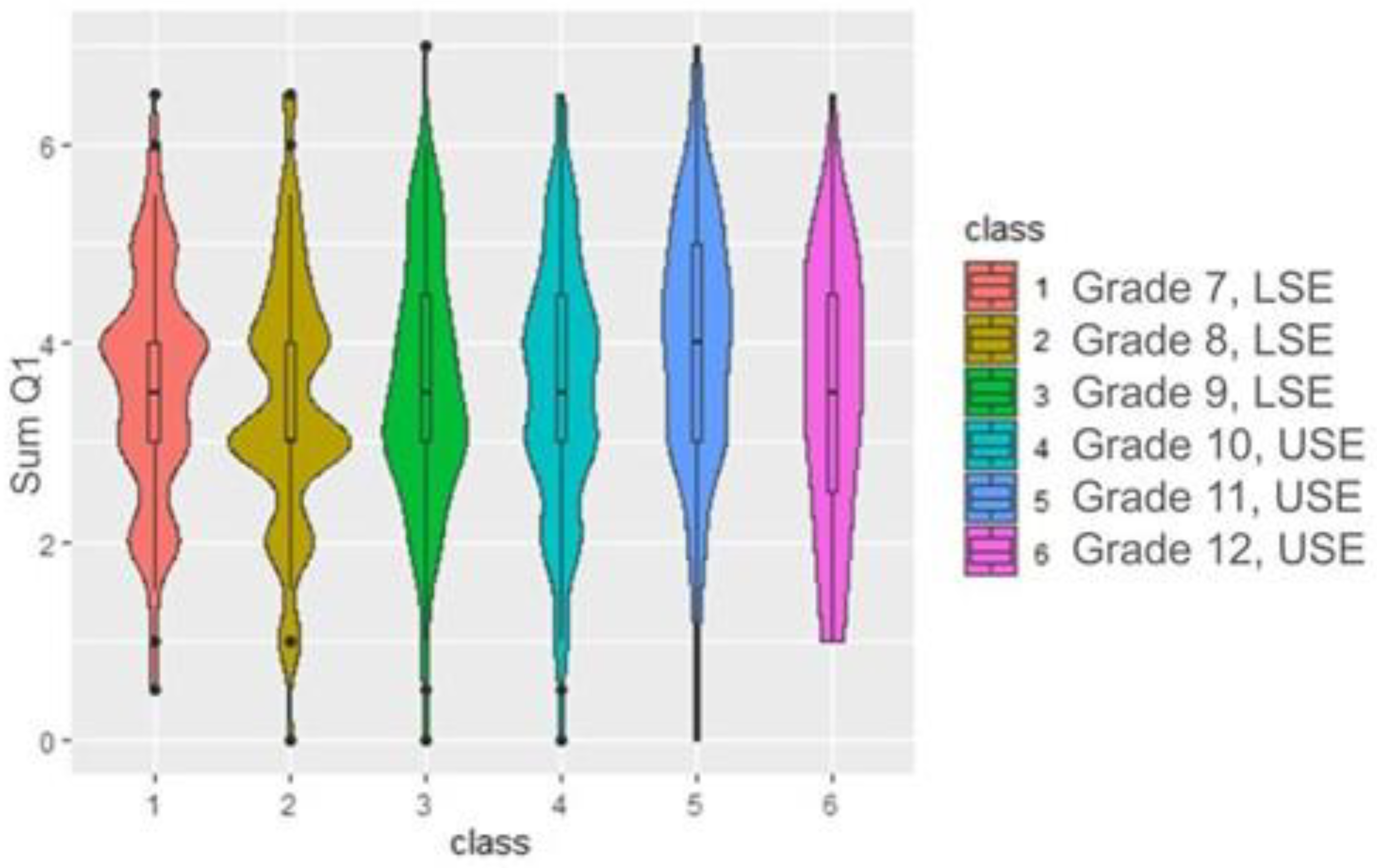
Thus, according to Figure 2 (SumQ1—Class) (where SumQ1 stands for Metals and Mineral–Rock Differentiation subcategories of questions as seen in Table 1) and the Mann–Whitney comparisons with Bonferroni correction (statistically significant, p = 0.001) the second grade of USE differs from all other groups. Also, the second grade of LSE differs from the second grade of USE based on median two schemes, but not with the rest. From the Figure 1 and the average values, it appears that the second grade of USEs has more correct answers regarding the questions related to Metals and Mineral–Rock Differentiation, compared to the rest of the classes.

In particular, the second grade of USEs, compared to the second grade of LSEs, has the maximum difference compared to all other classes.

Regarding the Q4 question group (Rocks) about the class attendance (Figure 3), according to the Kruskal–Wallis test, the p-value is statistically significant (0.001), with the median in all six (6) classes being around 3.

A Mann–Whitney comparisons test was performed, with Bonferroni correction, according to which there are statistically significant differences between the first grade of LSEs and the first and second grades of USEs, where USE students gave more correct answers (

Table 4. Pivot table of groups Q1 and Q4 for gender and class and p-value.

	Y-Axis	X-Axis	Kruskal–Wallis Control (p-Value)	Mann–Whitney (Bonferroni Corrected)
Figure 2	Q1 (Mineral–rock differentiation)	Class	0.0001404	Second grade of USEs differs significantly from the rest of the classes and gave more correct answers, especially compared to the second grade of LSEs.
Figure 3	Q4 (Rocks)	Class	0.001661	USE students gave more correct answers. Between the third grade and the second grade of USEs, the latter gave more correct answers.

Where bold means that the difference is statistically significant.

). Also, between the third grade of LSEs and the second grade of USEs, the latter gave more correct answers.

According to the above table, statistically significant differences were found in favor of the second-grade students in USEs, who performed significantly better than other student groups. This difference is particularly significant when compared to their peers in LSEs. Overall, USE students gave more correct responses, with second-grade USE students outperforming even those in the third grades of the same school type.

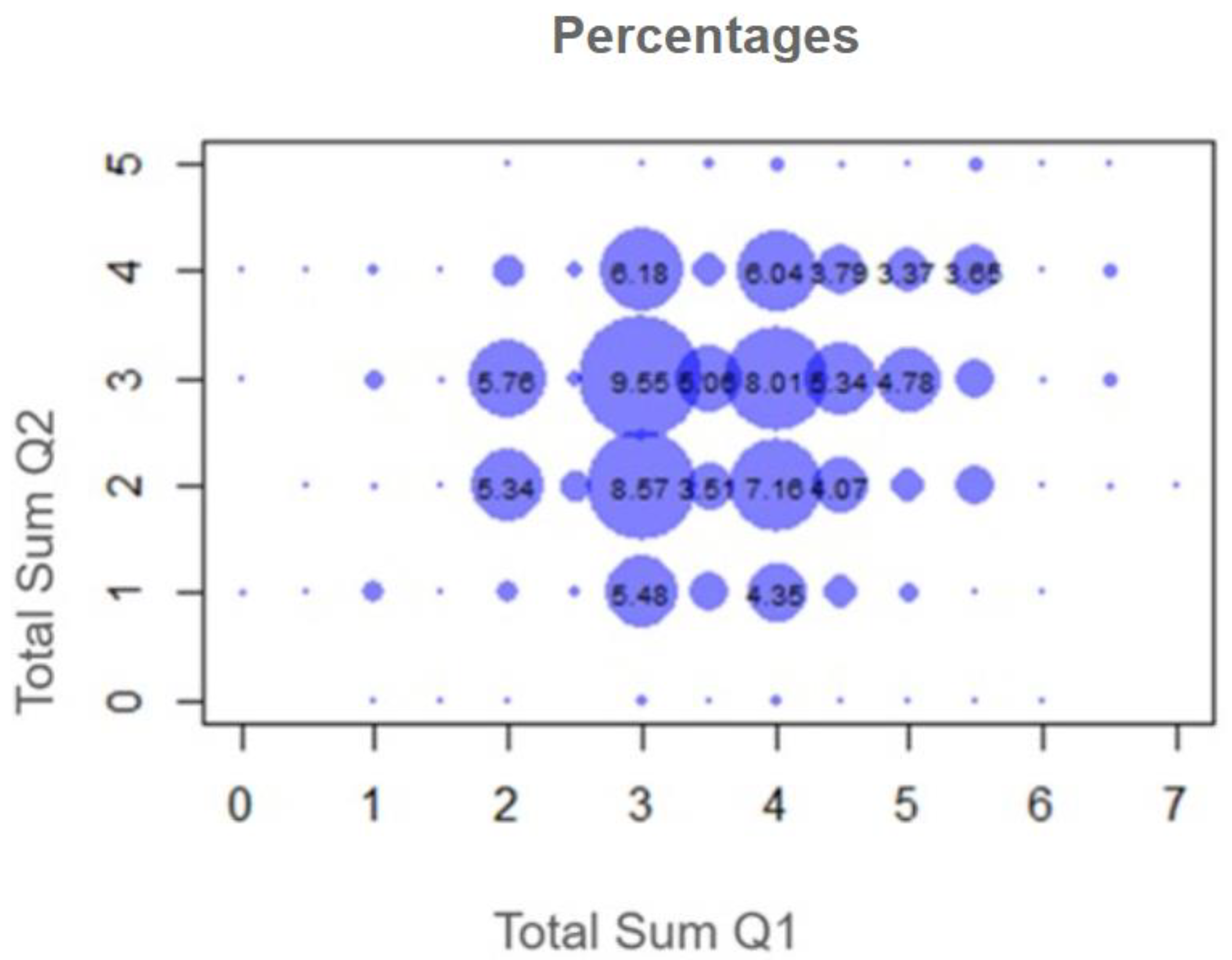
In Figure 4, a correlation between the number of correct answers in Q1 (Mineral–Rock Differentiation) and Q2 (Life Cycle) is presented.

According to Figure 4, the highest frequency (9.55%) is observed in the combination (3.3) for Q1 and Q2 number of correct of answers. Also, there seems to be a slight positive correlation since large values of Q1 are observed together with large values for Q2, and small values of Q1 together with small values for Q2. Students who answered correctly in the Q1 question category tended to answer correctly in the Q2 question category as well. Similarly, students who did not answer correctly in category Q1 did the same in category Q2. In any case, the majority of students answered with “moderate” accuracy, i.e., they fell between 3 and 4 in Figure 4.

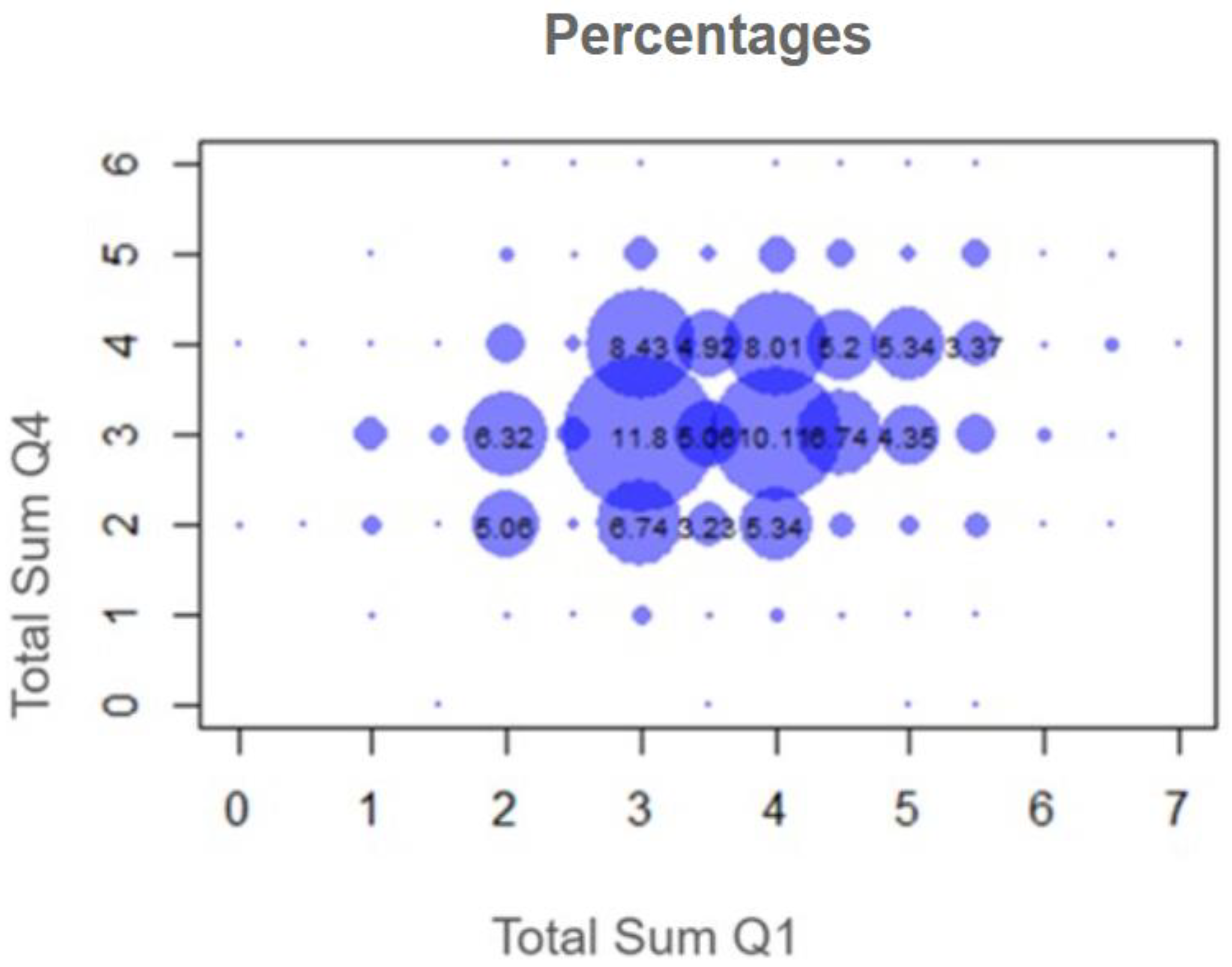
Figure 5 presents the results of a correlation conducted between the number of correct answers in Q4 (Rocks) and Q1 (Mineral-rock differentiation).

There is a positive correlation in Q4 = 3 and Q1 = 3 and 4. Also there seems to be a slight positive correlation, since large values of Q4 are observed along with large values for Q1, and small values of Q4 together with small values for Q1. In Figure 5, the majority of students answered with “moderate” accuracy, i.e., they fell between 3 and 4. Those who answered correctly in the Q1 category had a tendency to answer correctly in the Q4 category as well. Similarly, students who did not answer correctly in category Q1 did the same in category Q4.

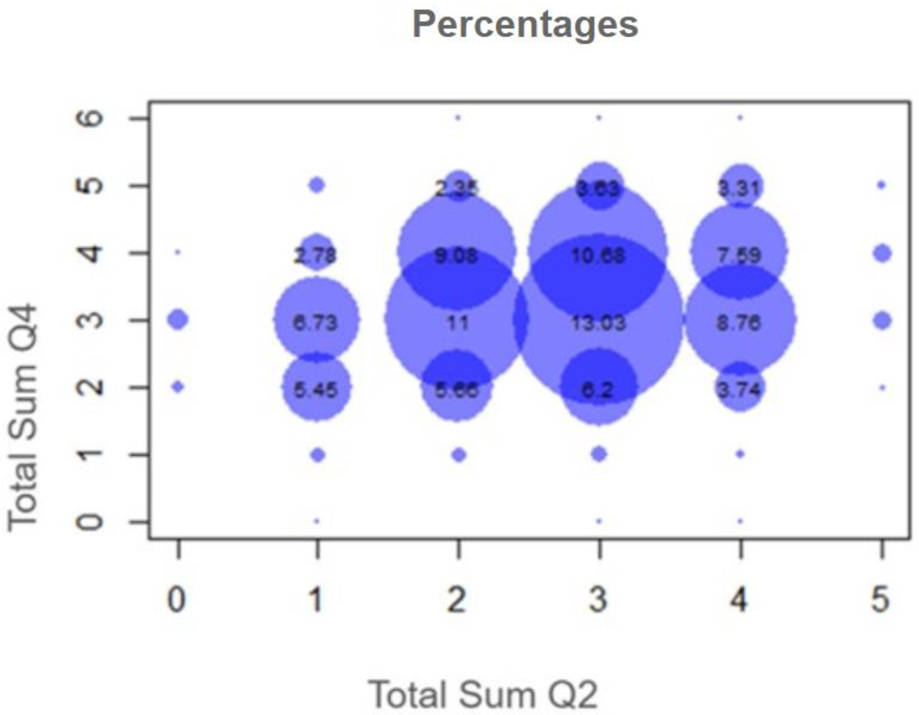
Figure 6 presents a correlation conducted between the number of correct answers Q4 (Rocks) and Q2 (Life Cycle).

There is a correlation between Q4 = 3 and Q2 = 2 through 4. Also, there seems to be a slight positive correlation, since large values of Q4 are observed along with large values for Q2, and small values of Q4 together with small values for Q2. Therefore, the majority of students answered with “moderate” accuracy, i.e., they fell between 3 and 4. Those who answered correctly in the Q2 question category had a tendency to answer correctly in the Q4 question category as well (values 11 and 13.03 in Figure 6).

In order to complement and enhance the aforementioned results,

Table 5. Correlation matrix for Total Sum Q1, Total Sum Q2, Total Sum Q3, and Total Sum Q4.

	Total Sum Q1	Total Sum Q2	Total Sum Q3	Total Sum Q4
Total Sum Q1	-
Total Sum Q2	0.151 *	-
Total Sum Q3	0.252 *	0.145 *	-
Total Sum Q4	0.208 *	0.176 *	0.214 *	-

*: p-value < 0.001.

reports the Spearman correlation matrix among the four categories under study. The analysis indicates the presence of a weak but consistently positive association across categories, which nevertheless reaches the threshold of statistical significance. This finding suggests that, although the strength of the relationships is limited, the correlations are not due to chance and warrant further consideration in the interpretation of the data.

3.4. Clustering

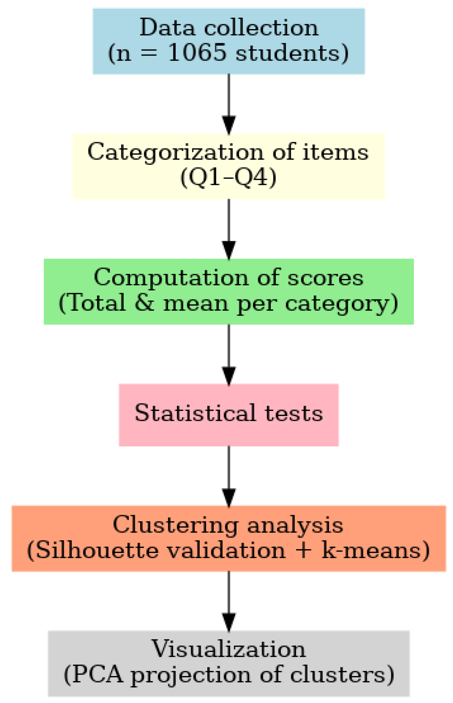
Clustering analysis was applied in order to identify groups of students with similar response patterns across the four main categories of misconceptions (Q1: Mineral–rock differentiation, Q2: Rock Life Cycle, Q3: Minerals, Q4: Rocks) and selected demographic variables (school type, city of residence, siblings, family background, and gender). For each category, the total score was calculated by summing the correct responses to the relevant items. These total scores, together with the demographic variables, served as the input for the clustering procedure (

Table 6. Mean value and standard deviation of Total Sums Q1: Mineral–rock differentiation, Q2: Life Cycle, Q3: Minerals, Q4: Rocks.

School	City	Mean of the Total Sum Q1	Mean of the Total Sum Q2	Mean of the Total Sum Q3	Mean of the Total Sum Q4	Standard Deviation of Total Sum Q1	Standard Deviation of Total Sum Q2	Standard Deviation of Total Sum Q3	Standard Deviation of Total Sum Q4
LSE	Patras	3.85	2.49	10.7	3.04	1.21	1.17	2.11	1.01
LSE	Outskirts of Patras	3.36	2.58	10.4	3.1	1.19	1.15	2.31	1.02
USE	Patras	3.79	2.77	10.7	3.32	1.31	1.18	2.39	1.03
USE	Outskirts of Patras	3.56	2.58	10.8	3.29	1.31	1.1	2.33	1.09

).

In order to construct cluster profiles, the following parameters were used: Total sum Q1, Total sum Q2, Total sum Q3, Total sum Q4, school, city, siblings, family, gender (Figure 7). Total Sums refers to the sum of the values of students’ responses in each category, e.g., the Total Sum Q1 refers to the sum of the values of the answers of the students who answered the Q1 question category, and so on.

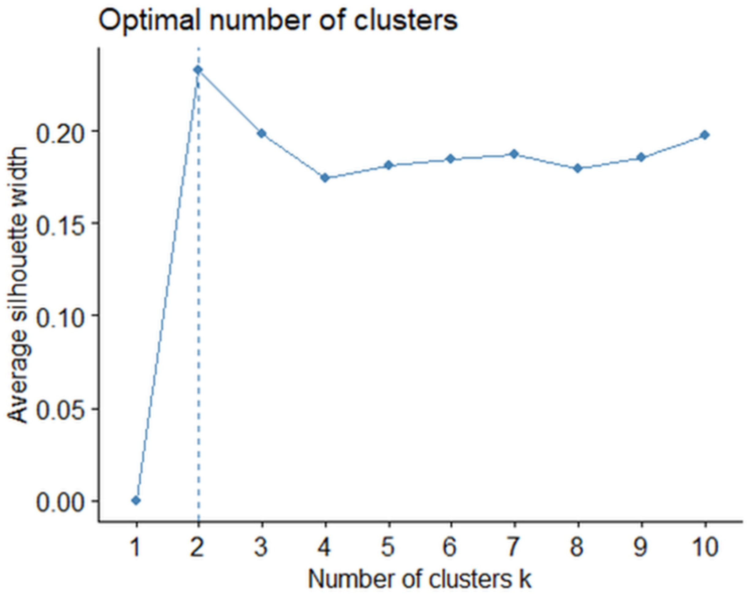
The optimal number of clusters was determined using the “Silhouette” method (Figure 7).

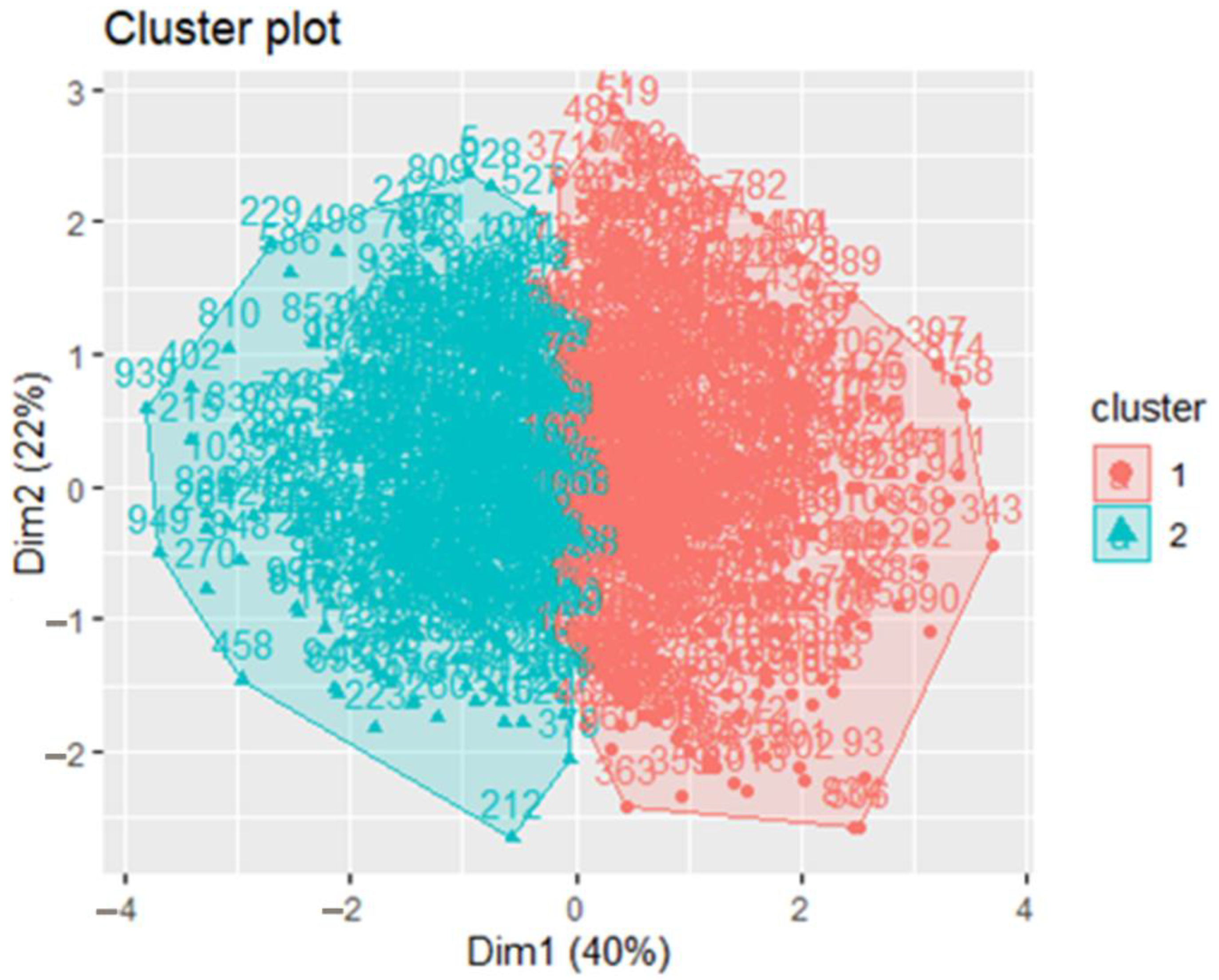
This method indicated that two clusters provided the best separation. Subsequently, k-means clustering was performed, and two distinct student profiles emerged. Cluster 1 included students with relatively higher performance across categories, while Cluster 2 consisted of students with comparatively lower scores. Figure 7 presents a visualization of the clustering results using principal component analysis (PCA), showing the distribution of students across the two clusters.

It is important to note that all four categories (Q1–Q4), including Q3, were incorporated in the clustering analysis, ensuring that the grouping reflects the combined performance across the entire set of questions. Finally, two clusters were created, based on the values Total Sum (Q1… Q4), as shown in

Table 7. Average values per cluster and Total Sum Q1, Total Sum Q2, Total Sum Q3, Total Sum Q4.

Cluster	Total Sum Q1	Total Sum Q2	Total Sum Q3	Total Sum Q4
1	3.01	2.14	9.45	2.66
2	4.28	3.20	11.90	3.84

. Cluster 1 mainly included students with overall higher performance across Q1–Q4, particularly in mineral–rock differentiation (Q1), whereas Cluster 2 consisted of students with lower scores across categories. Moreover, the distribution of students across the two clusters was not random: USE students were more frequently represented in both clusters, suggesting that school type contributed to the observed grouping.

Cluster Profiles

The profile of each group describes its hidden similarities and structures. Figure 8 shows the separation of clusters at the level of the first two principal components of Q1, Q2, Q3, and Q4 which, depending on their numerical value, are divided into two clusters. The two axes (Dim1 and Dim2) represent the first two principal components, which explain 40% and 22% of the total variance, respectively. Each point corresponds to an individual student projected in this reduced two-dimensional space, while colors indicate the two clusters obtained by k-means. The polygons delineate the area covered by each cluster, highlighting the separation between student groups. The PCA results revealed distinct clustering patterns among the Q1–Q4 question groups, highlighting clear differentiation in how students conceptualize minerals, rocks, and the rock cycle. This clustering underscores meaningful variations in students’ responses and supports targeted interpretation of domain-specific misconceptions. Principal Component Analysis is a well-established multivariate technique for reducing dimensionality by generating uncorrelated components that capture maximal variance––an approach frequently applied to geochemical and sedimentological datasets to interpret compositional stratigraphy [51].

The results are shown in detail in Table 7 below. In Cluster 2, where in all indicators the average value is higher, those who generally do better are concentrated.

Figure 9 below shows the two clusters and School type (LSE, USE). This Figure presents the distribution of students by School type (LSE vs. USE) within the two identified clusters. The results indicate that the clustering structure partially reflects school-related differences, with USE students being more represented in both groups.

The p-value (0.001) is statistically significant when testing independence between the two variables x² for cluster and school. The LSE has 404 students and the USE (USE, USVE, Other) 661 students. In clusters 1 and 2 (Figure 9), USE gathers more numerical values. As a percentage, however, blue is a little larger at 1 than it is at 2. This means that if an individual from High School is accidentally found, they are more likely, based on its characteristics, to join group 2.

Regarding the independence test between the clusters and School type (i.e., LSE and USE), the independence hypothesis is rejected, so it seems that there is a differentiation between LSE and USE between the two clusters, where more specifically, the second cluster gathers a higher percentage of the number of USEs compared to the first cluster.

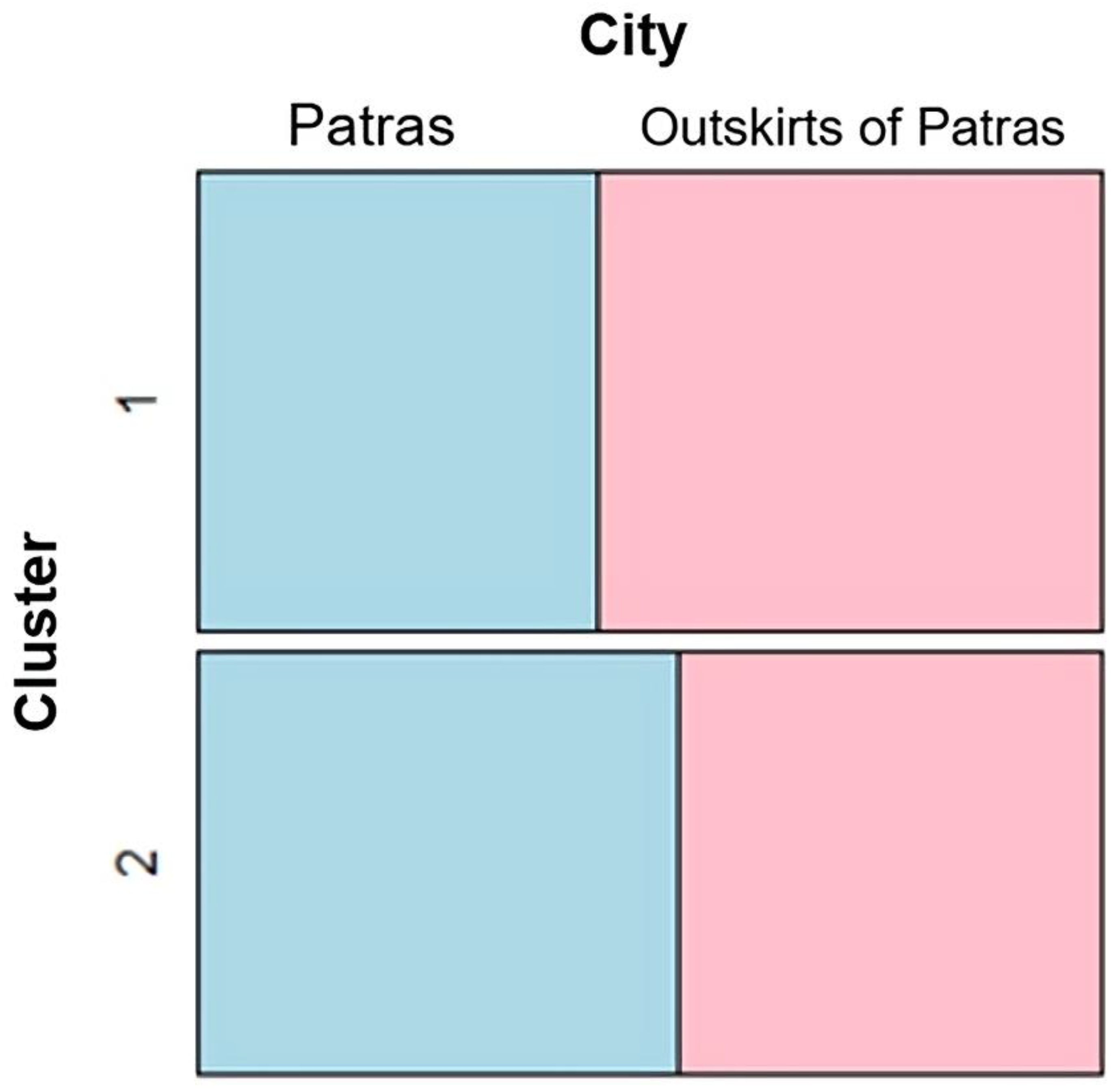
In “Patras”, 516 students participated, while “anywhere else in the prefecture of Achaia”, 549 students participated (Figure 10).

Here it seems that City is differentiated between clusters. City (Patras) and the rest of the regional unit of Achaia are not evenly distributed.

In cluster 1 (1st row) the blue part is much smaller than the blue part of the cluster in the 2nd row. (If City were not differentiated between the clusters, the figures in both graphs would be almost the same; however, in cluster 1, there are more values in the outskirts of Patras (549 responses).

Regarding the independence test between the clusters and the city (i.e., the urban center of Patras and all the other areas of the regional unit of Achaia), the independence hypothesis is rejected, so it seems that there is a differentiation between the urban center of Patras and all the other areas of the regional unit of Achaia between the two clusters, where more specifically the second cluster gathers a higher percentage of the number of areas outside the urban center of Patras in relation to the first cluster.

Parents’ marital status does not seem to play a role, as the values are similar (p-value = 0.625) (Figure 11). There were more indications of Parents staying together (792 responses) than for all other cases (separated, and more) (273 responses). Regarding the cluster in relation to gender (p-value = 0.069) and siblings, there does not seem to be significant statistical differences.

Finally, regarding the profile of the second cluster (

Table 8. Average values per cluster, School, City, and Total Sum Q1, Total Sum Q2, Total Sum Q3, Total Sum Q4.

Cluster	School	City	Total Sum Q1	Total Sum Q2	Total Sum Q3	Total Sum Q4
1	LSE	Patras	3.28	2.04	9.78	2.55
		Outskirts of Patras	2.97	2.16	9.46	2.65
	USE	Patras	3.01	2.14	9.25	2.69
		Outskirts of Patras	2.97	2.15	9.59	2.66
2	LSE	Patras	4.56	3.05	11.80	3.65
		Outskirts of Patras	3.94	3.20	11.80	3.77
	USE	Patras	4.46 *	3.30	11.90	3.85
		Outskirts of Patras	4.22	3.05	12.1	3.99

* Bold or larger numeric values in correct answers.

), they were USE students from Patras who demonstrated a higher score, i.e., they gave more correct answers, in: Total Sum Q1, Total Sum Q2, Total Sum Q3, and Total Sum Q4.

4. Discussion

The current research provided valuable insights into students’ misconceptions about basic concepts in geology, specifically regarding minerals and rocks. The first research question examined whether demographic characteristics, such as gender, place of residence, school, age, parents’ occupation, and parents’ marital status, contribute to the creation and the persistence of geological misconceptions. The results showed notable differences based on place of residence, i.e., between the urban center of Patras and all the other areas of the Achaia region. Clustering analysis of the questionnaire responses indicated that students from Patras consistently performed better in question category Q1 (Metals, Mineral–rock differentiation), highlighting an urban–rural divide.

4.1. Differentiation of Minerals and Rocks (Q1)

Both location (Patras vs. other areas outside Patras) and school type (LSE vs. USE) were found to influence students’ performance, especially in question category Q1. Students from USEs in Patras achieved the highest number of correct responses in Q1 and showed high performance in Q2 (Rock Life Cycle), as well as in Q4 (Rocks). On the other hand, schools outside Patras, regardless of level, scored lower in general. Additionally, the USE students of Patras consistently outperformed their peers, followed by the LSE students of Patras, who showed relatively high performance in category Q1.

Statistical analysis confirmed significant differences among student groups in Q1 and Q4 and based on their grade level. Specifically, in category Q1, second-grade USE students scored significantly higher than the second-grade LSE students, though not significantly different from other groups. Figure 2 further illustrates that first- and second-grade USE students outperformed first-grade LSE students, while second-grade USE students also outperformed third-grade LSE students. These findings suggest that both school types as well as location seem to play a key role in students’ geological understanding.

For questions c. “Can students distinguish minerals from rocks?” and e. “Can students distinguish geological time compared to the lifespan of a human on Earth and/or the total time of human presence on Earth?”, there is insufficient data to draw conclusions, although it could be further explored in a future study.

4.2. Predictive Factors

Regarding questions b. “Do demographic characteristics play a role in misconceptions about minerals?” and d. “Do demographic characteristics play a role in misconceptions about rocks?”, the results did not show any statistically significant differences between the groups in relation to family, gender, and siblings.

Both City and School emerged as significant factors in shaping students’ responses, particularly within the Q1 group of questions (differentiation of minerals and rocks). Thus, LSE and USE students residing in the City answered more accurately compared to those Outside the City. City is further associated with performance in Q2 (Rock Life Cycle), suggesting that students’ place of residence influences how they conceptualize long-term geological processes. Thus, along with USE students from the city, LSE students from outside the city also answer correctly.

Similarly, the School type is linked to Q4 (Rocks), indicating that institutional context affects students’ understanding of rock-related concepts. Taken together, the statistically significant p-values for Q1 and Q4 confirm that misconceptions are not randomly distributed but are systematically related to the class students attend.

Regarding the Q4 question group (Rocks) and class, there are statistically significant differences between the first grade of LSE and the first and second grades of USE, as well as between the third grade of LSE and the second grade of USE.

Current research shows that secondary school students have various misconceptions about minerals and rocks, as well as relationships and interactions with the human world. These misconceptions are common with those reported in the literature and, as hypothesized, they may arise from incorrect intuitive perceptions of how the natural world evolves, or from stereotypes and assumptions acquired from the family environment, or inadequacies in the school curriculum. Most of the participants in the study incorrectly believed that metals are hard (they have high hardness), that quartz is a rock, and that rocks are always solid. Many also held the false belief that soil is not rock and that rocks are created solely by catastrophic events, like earthquakes and volcanic eruptions. Additionally, students generally did not recognize hardness as a key property to identify rocks, nor that glass is not a mineral, and breaks easily. They also underestimated the impact of luster and brightness on the perceived color of minerals, and they were unaware that some rocks can be used as fuel. These misconceptions reflect the overall pattern of incorrect answers given by the majority of participants.

4.3. Geological Misconceptions in Secondary Education

These findings are consistent with international research indicating that misconceptions in the natural sciences, including geology, are not confined to specific regions but rather reflect a global phenomenon. A systematic review across multiple scientific domains highlights how misconceptions persist due to traditional, lecture-based teaching methods, emphasizing the need for inquiry-based and experiential approaches to foster conceptual change [49].

Moreover, educational studies focused on geology underscore the effectiveness of analogical teaching and hands-on, inquiry-based interventions in addressing persistent misconceptions, such as misunderstanding of geological time, rock formation processes, and material deformation [52].

These regional findings echo broader international evidence that student misconceptions about geological concepts, such as the distinction between minerals and rocks, are a widespread educational challenge. Innovative approaches, such as virtual mineralogical environments, have demonstrated potential for improving conceptual understanding globally by leveraging visual and interactive experiences [53].

It is worth mentioning that many of the above-mentioned topics where students hold misconceptions are not covered in the secondary school curriculum.

Table 9. Questionnaire items matched with syllabus of secondary education textbooks.

N/A	Category	Question	Second Grade of LSE	Page
1	Differentiation of minerals—rocks	Minerals and rocks do not have a significant role in our lives	Geography	39, 41
2	Minerals	A crystal cannot be scratched on glass if it is not a diamond	Chemistry	20
3	Minerals	There are rocks that are used as fuel	Geography	39
4	Rocks	Rocks are created by catastrophic events (earthquakes, volcanic eruptions)	Geography	39

shows the alignment between the concepts addressed in the questionnaire we used and the topics taught in each grade.

More specifically, Table 8 presents four selected questions which align with topics covered in the Geography and Chemistry curriculum of the second grade of LSE. It is evident that the first grade LSE students had not yet been taught the relevant material, while the third grade LSE students and all three grades of USE had covered the material, although retention may have diminished over time.

However, despite the misconceptions found in student responses, they also showed strong understanding in certain areas. Most of the participants correctly recognized that minerals and rocks play an important role in our lives, that liquids are not always light, and that rocks and minerals are not the same. Additionally, a majority of students correctly rejected the misconceptions that all rocks are the same, that all of them are heavy, and that a heavy mineral is also hard.

In relation to what students are taught, it must be noted that second grade LSE students performed relatively well, ranking just below second grade USE students, likely due to their recent exposure to related geological concepts. However, although first grade LSE students are taught basic geological concepts concerning minerals and rocks, their performance did not reflect this, since they ranked second-to-last in correct answers. Finally, the first grade USE students had the lowest performance overall, with very few correct answers.

4.4. Limitations and Further Research

This research could be extended to younger students, particularly those in the fifth and sixth grades of primary school, where basic geological concepts and phenomena are first introduced. Conducting studies at the primary level using questionnaires like the one used in this study would help identify early misconceptions, enabling timely and targeted instructional interventions. Addressing these misconceptions before students enter secondary education may prevent the persistence of inaccurate geological knowledge that often carries through to university-level studies.

Another important parameter involves the analysis of student responses to remote learning, providing insights that inform recommendations for enhancing future geological education through blended approaches that integrate traditional and digital methods [19].

Additionally, future research could be designed in alignment with the foundational principles of effective education as outlined by Bransford et al. [54]. These environments should be (a) student-centered, i.e., take into account students’ interests, (b) knowledge-centered, i.e., focus on what will be taught, why it will be taught, and what results it will produce, (c) focused on formative assessment, and d) connected to the community where the school is located. By using a questionnaire similar to the one used in the current study to evaluate students’ understanding both before and after the implementation of these educational strategies, researchers could assess the impact of structured, conceptually sound instruction on students’ comprehension of key geological topics and whether misconceptions on geology have been effectively addressed.

Further work is needed at both the K–12 and university levels, aimed at innovative approaches to address students’ perceptions of plate tectonics, including designing images that support key scientific messages. This research can inform curriculum development for entry-level geoscience courses as well as the use of images to transmit complex science [55].

5. Conclusions

The research examined misconceptions about basic geological concepts concerning minerals and rocks among secondary school students in the regional unit of Achaia. The findings revealed that students, particularly those attending USE schools and living on the outskirts of Patras, performed better in recognizing mineral-related concepts. However, a widespread lack of understanding was evident across all school levels, despite some of the content being included in the second-grade LSE Geography and Chemistry curriculum. At the same time, first-grade LSE students had not yet been exposed to this information, while third-grade LSE and all three grades of USE students likely struggled to recall it due to the time that had elapsed since instruction.

Common misconceptions included the belief that all metals are hard, that rocks are always solid, and that glass is a mineral. Students also showed confusion about mineral properties, like brightness and luster. These misconceptions highlight the significance of designing curricula that acknowledge and address students’ prior knowledge and misconceptions. It is a mistake to assume that students enter school tabula rasa. Instead, educators should recognize that students bring existing ideas––often incorrect and sometimes in conflict with scientific concepts––that must be challenged and reshaped through instruction, in line with the theory of conceptual change [2].

This study highlights the need for training secondary school science teachers, especially in geological topics, to effectively address student misconceptions. Ultimately, adapting teaching methods to recognize and tackle student misconceptions will enhance their understanding of science and geology. This strategy will not only promote personal cultural growth but also establish a strong foundation for students aiming to pursue a university degree in these fields.

In addition, we suggest that potential solutions could include the design of targeted teaching units, the use of interactive digital tools, field-based activities, and inquiry-based learning approaches tailored to students’ age and prior knowledge. These strategies can help address and gradually correct misconceptions about minerals, rocks, and the rock cycle.