Article

Machine Learning-Driven Calibration of MODFLOW Models: Comparing Random Forest and XGBoost Approaches

by
Husam Musa Baalousha
Department of Geosciences, College of Petroleum Engineering and Geosciences, King Fahd University of Petroleum and Minerals (KFUPM), Dhahran 31261, Saudi Arabia
Geosciences 2025, 15(8), 303; https://doi.org/10.3390/geosciences15080303
Submission received: 2 June 2025 / Revised: 22 July 2025 / Accepted: 30 July 2025 / Published: 5 August 2025
(This article belongs to the Section Hydrogeology)

Abstract

The groundwater inverse problem has several challenges such as instability, non-uniqueness, and complexity, especially for heterogeneous aquifers. Solving the inverse problem is the traditional way to calibrate models, but it is both time-consuming and sensitive to errors in the measurements. This study explores the use of machine learning (ML) surrogate models, namely Random Forest (RF) and Extreme Gradient Boosting (XGBoost), to solve the inverse problem for the groundwater model calibration. Datasets for 20 hydraulic conductivity fields were created randomly based on statistics of hydraulic conductivity from the available data of the Northern Aquifer of Qatar, which was used as a case study. The corresponding hydraulic head values were obtained using MODFLOW simulations, and the data were used to train and validate the ML models. The trained surrogate models were used to estimate the hydraulic conductivity based on field observations. The results show that both RF and XGBoost have considerable predictive skill, with RF having better R2 and RMSE values (R2 = 0.99 for training, 0.93 for testing) than XGBoost (R2 = 0.86 for training, 0.85 for testing). The ML-based method lowered the computational effort greatly compared to the classical solution of the inverse problem (i.e., using PEST) and still produced strong and reliable spatial patterns of hydraulic conductivity. This demonstrates the potential of machine learning models for calibrating complex groundwater systems.

Graphical Abstract

1. Introduction

Groundwater modeling is a powerful tool for water resource sustainability, management, and protection. To obtain reliable results of a developed model, accurate calibration is necessary, which is a significant challenge because model calibration involves solving an inverse problem, which is ill-posed [1,2,3].
The heterogeneous nature of aquifers is one of the main challenges in groundwater modeling and calibration [4,5]. The accurate characterization of hydraulic properties such as hydraulic conductivity and storage coefficients is essential for modeling; however, these parameters have a high spatial variability, especially in some geological settings like karst [6,7]. Calibration processes require solving an inverse problem, which aims to reduce the differences between model predictions and field observations by adjusting the parameters being calibrated [8]. If models are not properly calibrated, they might generate predictions that seem reasonable but are actually wrong, which will potentially lead to poor water management choices [9,10].
The calibration process of a groundwater model is inherently ill-posed [2,11,12]. The problem manifests in two ways: first, various parameter sets can produce nearly identical model predictions (non-uniqueness), and second, minor changes in data can lead to significantly different parameters, which is known as instability [6,12,13]. In addition, the high dimensionality of the calibrated parameter, which is the case in a highly heterogeneous aquifer, complicates calibration efforts [14]. Other issues such as field data limitations and measurement errors make the calibration process even more complicated [15].
Various methods have been developed to cope with the inverse modeling challenges discussed above. The PEST (parameter estimation and uncertainty analysis) is one of the most widely used tools for model calibration, which was developed by Doherty [16]. The PEST is a model-independent tool and can be coupled with any model such as the USGS modular groundwater (MODFLOW) model. PEST uses the Gauss–Marquardt–Levenberg method for optimization, regularization techniques to address ill-posed inverse problems, and singular value decomposition to reduce dimensionality and achieve a stable solution [17].
The pilot point method is one of the most widely used methods for characterizing spatial heterogeneity and for reducing the number of parameters [17]. This method uses the interpolation (e.g., kriging) between a finite number of points within a model domain to create continuous parameter fields [18]. The advantages of the pilot points method is the significant reduction in the number of calibrated parameters while maintaining the general spatial characteristics. Other methods include the zonation method, which divides the model domain into areas of uniform properties [19], and ensemble methods, such as the Ensemble Kalman Filter, which uses many realizations to characterize uncertainty [20].
Despite the significant advancement in the development of model calibration methods, there are still many important limitations. One of these limitations is the computational expenses required for calibration, which can be prohibitive [21]. The problem becomes even more complicated when performing an uncertainty analysis for the highly parametrized problems [1,22,23]. In addition to computation expenses, the non-uniqueness problem is another significant challenge in the inverse problem [6]. It has been shown that various solutions of independent parameters can be a solution for the inverse problem with the same accuracy. Baalousha [1] assessed the uncertainty in the calibrated hydraulic conductivity resulting from the non-uniqueness of the solution for the inverse problem. Some researchers introduced certain techniques to overcome the non-uniqueness issue. These techniques include using prior information and regularization to constrain the solution [9,24].
Recent developments in machine learning (ML) demonstrate promising alternatives to the previously mentioned techniques for groundwater model calibration [25,26,27]. Surrogate models have been widely used in hydrogeology, i.e., [28,29,30]. These models utilize the data-driven approaches to understand the complex non-linear relationship between dependent and independent variables of complex models [31,32]. Random Forest (RF) uses ensemble decision tress to make reliable predictions and importance rankings [33]. XGBoost uses gradient boosting methods with regularization to increase the predictive accuracy of the models [34,35].
To the best of our knowledge, no research has been published on inverse modeling using ML tools. Therefore, this study is considered a pioneering work and an introduction to the use of AI methods in inverse modeling. This paper proposes training a surrogate model on a limited number of MODFLOW simulations (20 runs) to predict the groundwater head based on various inputs of the hydraulic conductivity field. The trained models are then used to calibrate the model, and the results are compared with the classical model calibration using pilot points from a previous study. Two ML models are considered in this study: the RF and XGBoost. The case study where the models are developed is the Northern Aquifer of Qatar.

2. The Study Area and Its Geology

Qatar is one of the Gulf Cooperation Council (GCC) states, located in the eastern part of the Arabian Peninsula. It is surrounded by the Arabian Gulf and borders Saudi Arabia in the south, as shown in Figure 1. The total area of Qatar is approximately 11,500 km2, and its climate is very arid with a long summer and mild winter. The long-term average annual precipitation is less than 80 mm, whereas the potential evapotranspiration is more than 2200 mm [36]. The topography of the country is generally flat, with some high terrain in the southern part, which reaches approximately 100 m above the mean sea level.
The study area is the Northern Aquifer of Qatar, Figure 1. The area was selected because modeling work has been performed in this area [1], and the data is readily available through various publications, i.e., [37,38,39,40]. The surface geology of the Northern Aquifer comprises Dammam and Rus Formations from the Eocene. The Rus Formation with the underlying Umm er Radhuma Formation are the main aquifers in the country. These formations are composed of limestone and dolomite. Beach sediments and sabkhas (i.e., salt flat) occur along the coastal areas. The Northern Aquifer has a relatively good water quality compared to the southern one due to its geological settings. The lower Eocene Rus Formation contains a layer of gypsum in the southern aquifer, and this layer is highly soluble, resulting in the deterioration of the groundwater quality in that aquifer [37,41]. However, the gypsum layer is absent in the Northern Aquifer, which helps maintain a good water quality.
Aquifers are the only natural source of groundwater, which are highly exploited for agriculture, whereas the domestic water demand is met by desalination [42]. The average annual groundwater abstraction is 250 million m3, whereas the groundwater recharge varies between 10 and 166 million m3 per year [43]. The distribution of the groundwater recharge varies, with a higher recharge occurring in land depressions [44,45,46].

3. Materials and Methods

3.1. Methodology

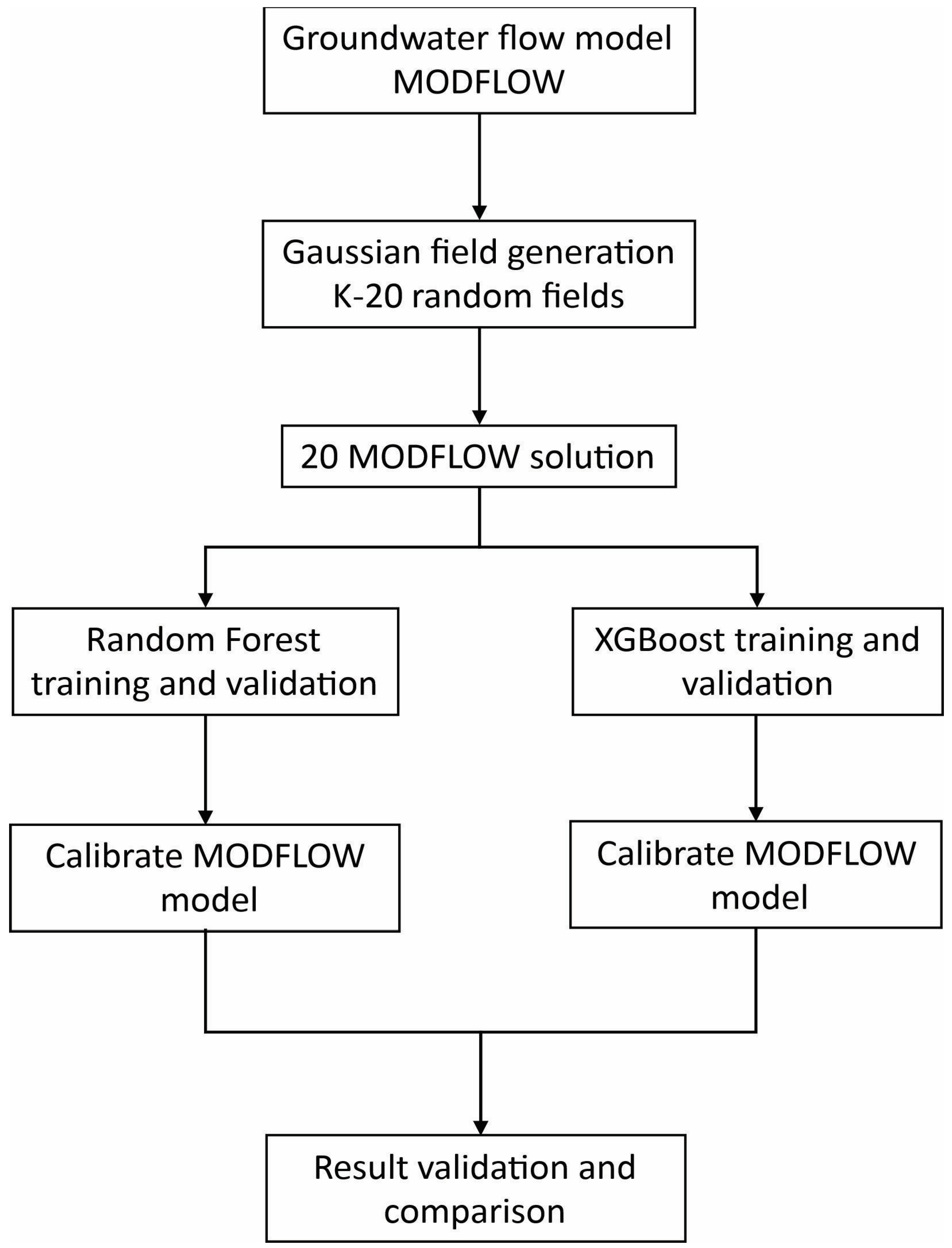
The stepwise methodology of this research is shown in Figure 2. The groundwater flow model was based on previous work performed by [1], which is based on the finite difference USGS MODFLOW model [47]. Twenty datasets were considered for training and validating the ML models. While the size of the training dataset may be questionable, this study aims to explore the use of a limited dataset. If the training dataset is large, it may render the use of ML tools non-competitive compared to traditional inverse modeling methods. The first step is to obtain 20 solutions of MODFLOW, using 20 matrices of hydraulic conductivity, the parameter being calibrated. These 20 matrices were obtained using stochastic random generator, as explained in the following section. Using these hydraulic conductivity matrices (K-20 matrices), the groundwater flow model was run for each, and 20 hydraulic head solutions were obtained (20 MODFLOW solutions). Two ML models, namely RF and XGBoost, were developed, trained, and validated using the 20-MODFLOW solutions. Both RF and XGBoost models were then used individually to calibrate the hydraulic conductivity in the MODFLOW model. Results are compared with the calibration obtained using the traditional PEST method.

3.2. MODFLOW Model

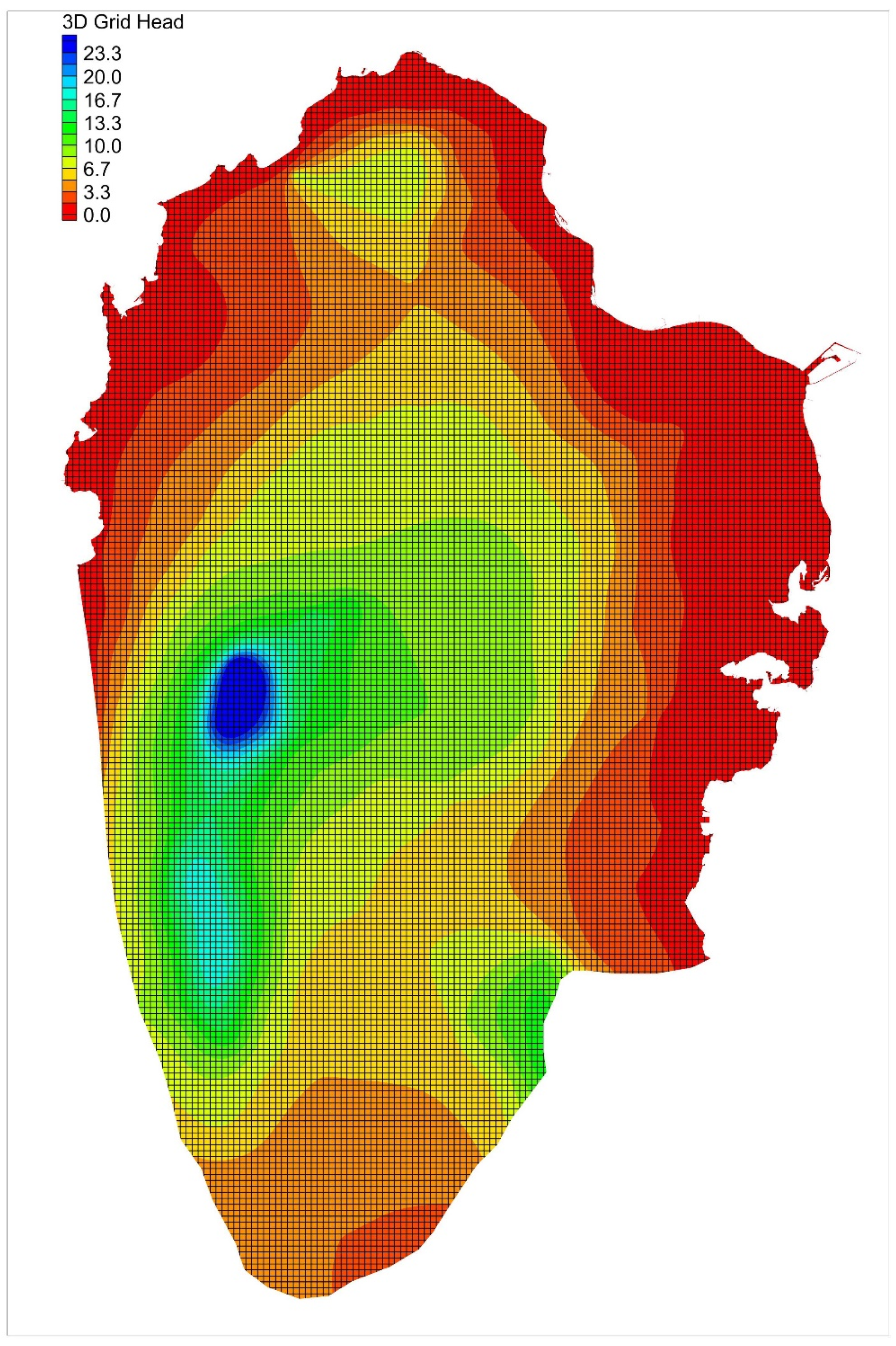
The model covers the Northern Aquifer, as shown in Figure 3, which has a total area of approximately 4300 km2. The model comprises 222 rows and 148 columns, with grid resolution of 500 m in both x and y directions. The aquifer is surrounded by the Arabian Gulf on all sides except the south. As such, constant head boundaries were assigned to eastern, northern, and western boundaries, and no-flow boundary was assigned to the south. Steady-state conditions were assumed to represent the case of pre-development conditions when groundwater abstraction was minimal. The available groundwater level data refers back to 1958 and was used to calibrate the model [1]. The hydraulic conductivity calibration using PEST was performed by [1] and is reproduced in Figure 3.

3.3. Machine Learning Models

3.3.1. Random Forest Model

RF is an ensemble machine learning (ML) method that was proposed by [48] and later extended by [33]. RF relies on building multiple decision trees using random subsets of the training data and can be used either for regression or data classification. For regression, RF outputs the average prediction of all decision trees, and for classification, it selects the most common class among the trees. Its main principles include bootstrap aggregating (bagging) and random feature selection at each tree split [48]. The advantages of RF are its ease of use, no overfitting, and good accuracy. In addition, it can handle high-dimensional data and cope with missing values [49,50].
In this study, an RF regression model was developed and trained on the 20 datasets of hydraulic heads produced by MODFLOW model, as explained in the methodology. The model was later used to predict hydraulic conductivity using the observation head data (i.e., solving the inverse problem).
The RF model was enhanced with some feature engineering to improve its performance. The feature engineering techniques include adding some additional variables, such as the square of hydraulic head, and the log-transformed head values. In addition, the location of each cell (i.e., column, row) was considered to capture any non-linear relationship between hydraulic head and hydraulic conductivity.
In this study, several feature engineering methods were used. A polynomial feature was used to capture non-linearity of the groundwater model, which is a well-known issue in groundwater modeling. A logarithmic transformation feature was used because some variables such as hydraulic conductivity are always positive. In addition, the log-normal transformation helps stabilize the problem. The spatial variability was addressed by considering column and row numbers to account for heterogeneity, which is very common in most aquifers.
Input data are the hydraulic conductivities produced by the random generator and the corresponding groundwater head produced by MODFLOW. The data is split into 80% for training and 20% for validation. The RandomForestRegressor library in Python 3.12 was used to train the model using 100 trees, and the model performance was assessed using mean absolute error (MAE), root mean squared error (RMSE), and the coefficient of determination (R2) on both training and testing datasets. The MAE measures the average absolute difference between the predicted and actual values as follows:
M A E = 1 N i = 1 N y i y ^ i
Similarly, the RMSE measures the square root of the average squared difference between the predicted and actual values and is given by
R M S E = 1 N i = 1 N y i y ^ i 2
The trained model was then used to predict the hydraulic conductivity using field measurements of groundwater head (i.e., steady-state head data).

3.3.2. XGBoost Model

The second machine learning model used in this study was XGBoost, which is the abbreviation of Extreme Gradient Boosting. Similarly to RF, XGBoost can be used for solving regression, classification, and ranking problems by combining the output of individual trees [34]. However, XGBoost builds decision trees in parallel and uses boosting to combine decision trees sequentially. In this study, the developed XGBoost model contains various components including data preprocessing, multi-target regression, hyperparameter optimization, and robust model evaluation protocols. This ensures the capture of reliable predictive relationships between hydraulic head and hydraulic conductivity.
The process starts with hydraulic head and hydraulic conductivity data reading and screening. The preprocessing includes standardization of all input variables so that all variables have the same range or distribution. This improves model stability and training speed. Logarithmic transformation was used to avoid negative values prediction for hydraulic conductivity.
The XGBoost model used hyperparameter optimization with 3-fold cross-validation. That is, the dataset is split into three parts where the model trains on two parts and validates on the third, rotating through all combinations. This process enables us to assess the performance more reliably and avoid overfitting.
The parameter space explored included tree-specific parameters, learning control parameters, regularization parameters, and tree construction parameters. Early stopping mechanisms were used during training to prevent overfitting and to optimize computation.

4. Results

4.1. RF Model Results

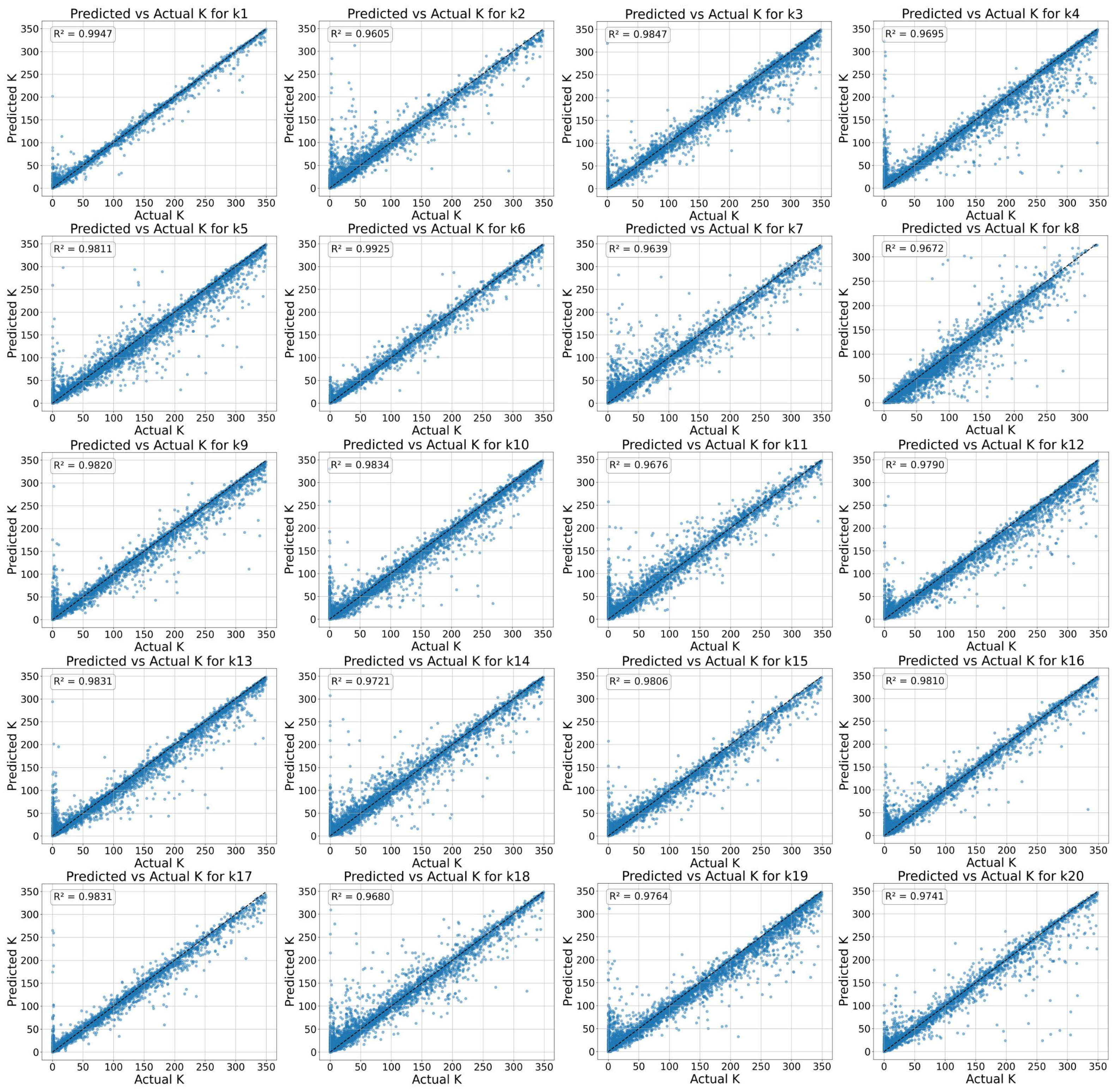
The resulting hydraulic conductivity is the one sought after, as it represents the calibration result. Model performance measures are shown in Table 1. Figure 4 shows the scatter plot of the predicted and trained hydraulic conductivity data for the 20 datasets. Results show that the coefficient of determination between predicted and actual hydraulic conductivity values is 0.99 for the training and 0.92 for the testing. The individual training of datasets shows that all coefficients of determination are above 0.94, as shown in Figure 4. For all of the 20 datasets, the coefficient of determination is above 0.9, which is a good indication of the robustness of the RF model and good training/validation results.
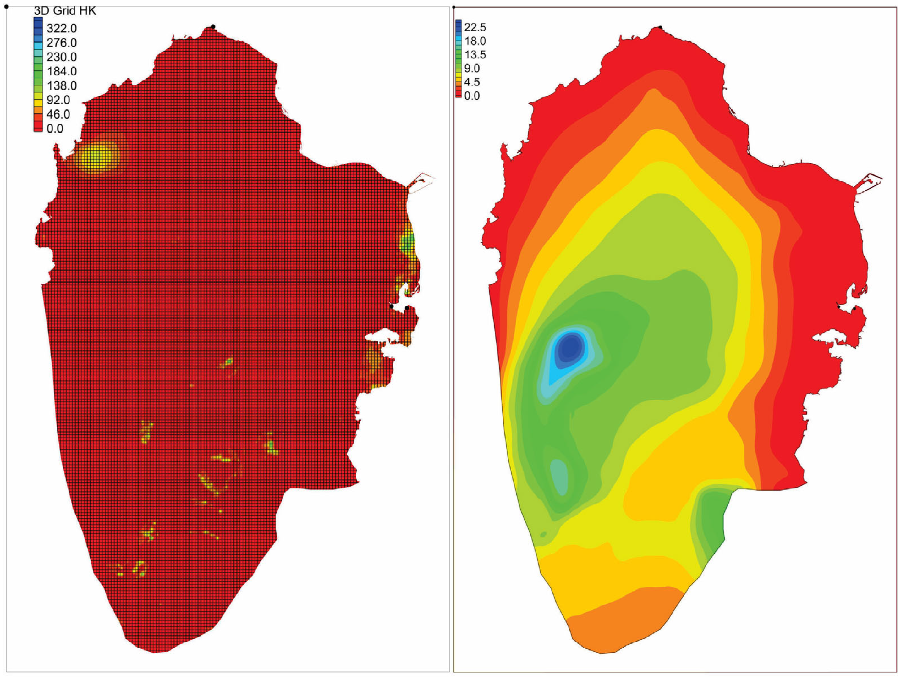
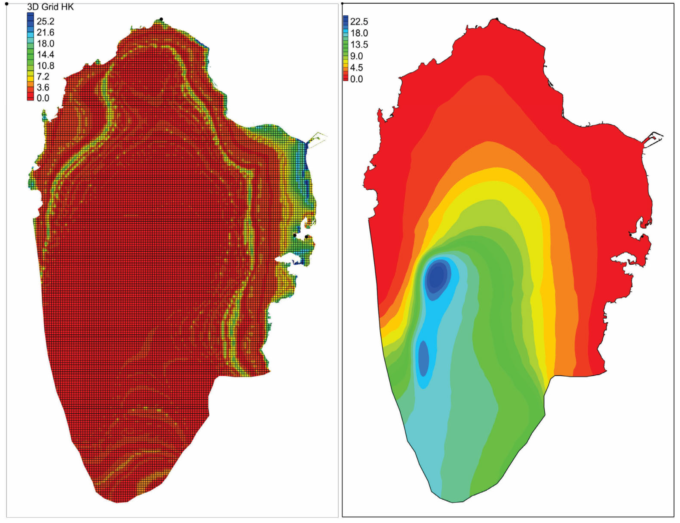
The trained RF model was used to predict the hydraulic conductivity, and the observation hydraulic head data were used as the input. These observations represent the steady-state conditions of the groundwater. This data refers back to 1958, when the groundwater abstraction was negligible, so it is fair to assume steady-state conditions [37]. The predicted hydraulic conductivity map and the corresponding hydraulic head are shown in Figure 5.
Hydraulic conductivity values vary between near 0 and 322 m/d, and high values occur in the eastern and southern part of the aquifer, in addition to one area in the west.
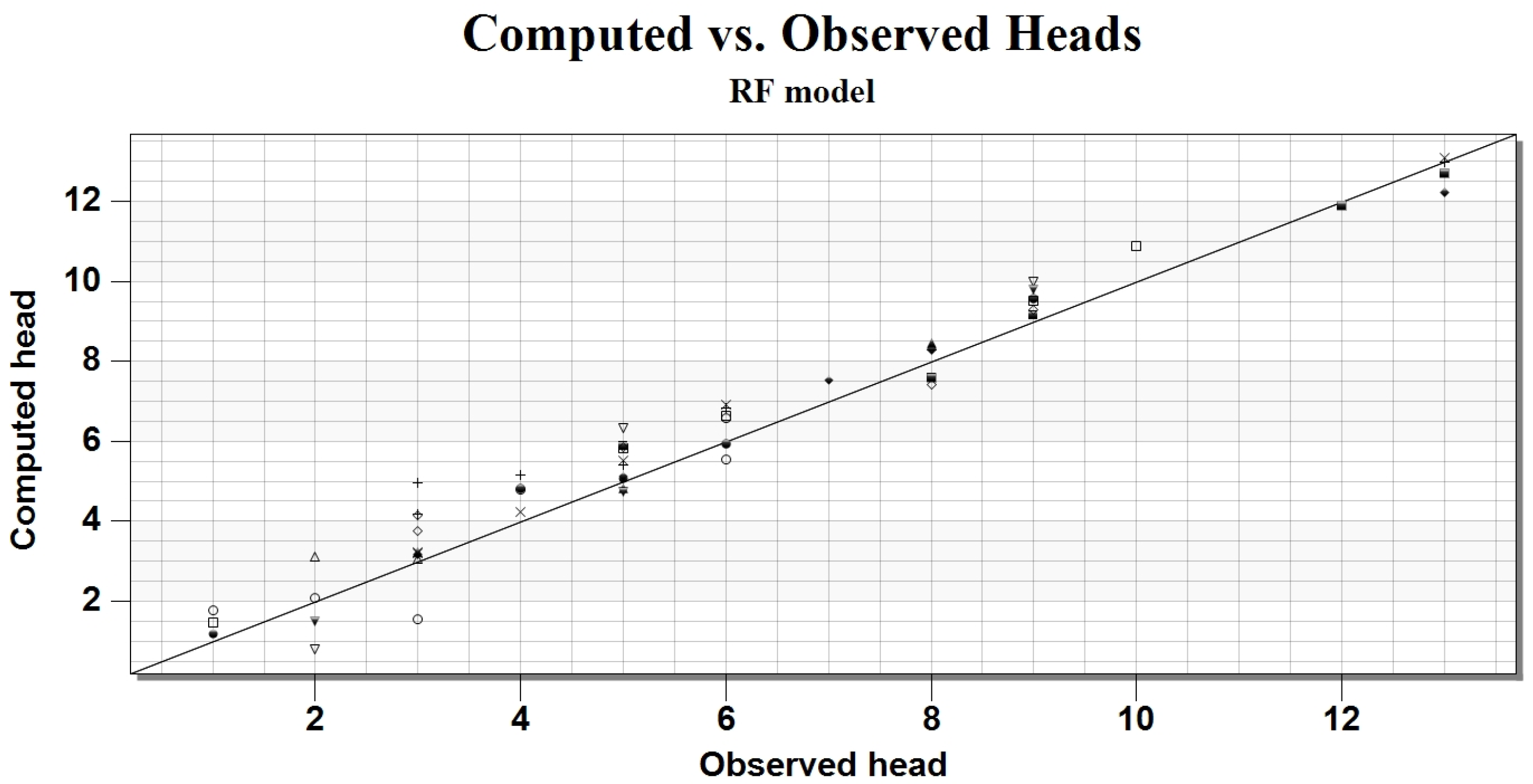
Figure 6 shows the calculated vs. observed head, using the head data obtained by the RF model. The figure shows small residuals, which indicate a good calibration. This is also confirmed by the error metrics shown in Table 1.

4.2. XGBoost Model Results

Similarly to the RF model, the XGBoost model performance was assessed using the Mean Absolute Error (MAE), Root Mean Square Error (RMSE), and coefficient of determination (R2). Figure 7 shows the scatter plot of the predicted and actual hydraulic conductivity in the training and validation process. While it is good in general, it is not as good as the RF. The coefficient of determination is above 0.8 for the majority of the dataset, except for datasets 2 and 7, where it is above 0.7. The overall error metrics for the XGBoost training are shown in Table 2.
Results show that the coefficients of determination between the predicted and actual hydraulic conductivity are 0.86 for the training and 0.85 for the testing. This indicates the good performance of the model. However, the overall performance is not as good as that obtained using RF, as indicated by the RMSE and MAE.
The trained XGBoost model was used to predict the hydraulic conductivity, and the observation hydraulic head data were used as the input. The resulting hydraulic conductivity map and the corresponding hydraulic head are shown in Figure 8. While both RF and XGBoost models successfully predict the hydraulic conductivity fields with a reasonably good accuracy, the results are significantly different. The hydraulic conductivity resulting from XGBoost is much lower, with a different spatial distribution than that resulting from the RF model. The hydraulic conductivity values in the XGBoost model vary between near 0 and just over 25 m/d, with a higher variability compared to those resulting from the RF model. Both, however, reproduce the groundwater level with a reasonably good accuracy, though RF has a higher accuracy. In both cases, a higher hydraulic conductivity occurs in the eastern side of the model area.
Figure 9 shows the calculated vs. observed head, using the head data obtained by the XGBoost model. Obviously, the residuals are larger than those obtained using the RF model. This is also demonstrated by the error metrics shown in Table 2.
In RF and XGBoost, the feature importance quantifies the degree to which each feature helps the model generate accurate predictions. It helps determine which factors have the highest impact on the model output. The results of the feature importance analysis of features used in both RF and XGBoost models are shown in Table 3. For both models, the row number was found to have the highest importance followed by the column. This highlights the importance of the location, more than anything else, for the predicted value of the hydraulic conductivity.

5. Discussion

In this study, ML models, namely RF and XGBoost, were developed to calibrate a groundwater flow model. It is noted that RF has a higher accuracy and requires less time to train the data of the study area, which is the Northern Aquifer of Qatar. The structures of RF and XGBoost models are totally different, which affects their performance, suitability, and accuracy. The RF model uses parallel learning, where each decision tree trains independently, while XGBoost uses sequential learning, where each tree tries to correct the previous one. The bagging mechanism of RF reduces overfitting and provides more stable predictions, which is beneficial when working with limited training data, as in this study (20 datasets). On the other hand, XGBoost follows a sequential boosting approach, which makes it more affected by noise and outliers in the groundwater data, leading to less robust predictions. RF performs much better with R2 values of 0.99 (training) and 0.93 (testing) compared to XGBoost, which has R2 values of 0.86 (training) and 0.85 (testing). The RMSE values also are better in the case of RF (4.7 training, 12.93 testing) compared to XGBoost (22.1 training, 23.3 testing). The feature importance analysis shows that both RF and XGBoost models rely more on row and column coordinates (spatial location) than the actual hydraulic head values as predictive features. This may raise concerns about overfitting; however, since the discrepancy between the training and testing performance metrics is small, overfitting can be excluded. The high importance of the spatial location reflects the heterogeneous nature of the aquifer, because of the high variability of the hydraulic conductivity as demonstrated by the pumping test data [51].
It is noted that there is a significant difference between RF and XGBoost in the spatial distribution and magnitude of the predicted hydraulic conductivity spatial distributions, although both models fairly reproduced the groundwater head. The RF model predicted hydraulic conductivity values ranging from near 0 to 322 m/d, while XGBoost predicted a much narrower range of 0 to 25 m/d.
This difference in the results of both models is not surprising, as the inverse groundwater modeling is ill-posed, which means the solution is non-unique.
Both models found higher hydraulic conductivity zones in the eastern part of the study area, which aligns with the geological understanding of the Northern Aquifer of Qatar. However, the magnitude differences show that model selection and validation methods must go beyond simple performance metrics to include geological plausibility and physical constraints.
The ML-based methods have significant computational benefits. Iterative forward model runs and sensitivity calculations are necessary for the traditional PEST calibration, which can be computationally prohibitive for highly parameterized models. Although the training takes considerable time, after training, the ML surrogate models produce predictions quickly, which enables quick scenario testing and uncertainty analyses that would be otherwise difficult with traditional methods.
Future work might include a hybrid approach that incorporates ML models and traditional approaches such as the PEST. The ML approaches could be used as a starter to narrow down the search for optimal values, and the PEST can be used to fine-tune the results. This combination can significantly reduce the computational expenses of the inverse problem. In all cases, there is a need to overcome the non-uniqueness issue, as it persists in all approaches, as the inverse problem is inherently ill-posed [1,2,3]. One way to address this is through prior information, such as the pumping test data, and homogeneity assumptions in addition to the expert knowledge of the particular area being studied.

6. Conclusions

This study demonstrates that ML surrogate models can effectively calibrate groundwater flow models with significantly reduced computational requirements compared to traditional inverse modeling approaches. The resulting hydraulic conductivity fields from both models differ, although both calibrate the model reasonably well. In both cases, the eastern part of the model has a high hydraulic conductivity, which is consistent with previous studies. As for efficiency, results showed that the RF model performs better than the XGBoost in predicting hydraulic conductivity fields, with R2 values of 0.99 for training and 0.93 for testing. Therefore, RF was found to have an excellent capability for this application. The use of ML models required significantly less time than traditional methods such as the PEST, which is useful for highly non-linear complex models. There is a need to enhance the ML predictability by incorporating additional information, such as the pumping test data, and prior information that helps overcome the non-uniqueness issue.
To create the training dataset for ML models, many MODFLOW runs are still necessary. The selection of 20 training datasets in this study aims at striking a balance between reducing computation expenses and having a good model performance. Future studies should explore the ideal number of training simulations for various aquifers with various complexities.
Although this study has successfully solved the inverse problem, it has limitations. There is a need to investigate the effect of the number of the training datasets on the accuracy of the results and the training time. A limited dataset may not fully capture the stochastic variability of the hydraulic conductivity field. Increasing the dataset may increase the run time, which is one of the main advantages of using ML for calibration.

Funding

Thanks for King Fahd University of Petroleum and Minerals (KFUPM) for supporting this research.

Data Availability Statement

The raw data supporting the conclusions of this article will be made available by the authors on request.

Conflicts of Interest

The authors declare no conflicts of interest.

References

  1. Baalousha, H.M. Predictive uncertainty analysis for a highly parameterized karst aquifer using null-space Monte Carlo. Front. Water 2024, 6, 1384983. [Google Scholar] [CrossRef]
  2. Carrera, J.; Alcolea, A.; Medina, A.; Hidalgo, J.; Slooten, L.J. Inverse problem in hydrogeology. Hydrogeol. J. 2005, 13, 206–222. [Google Scholar] [CrossRef]
  3. McLaughlin, D.; Townley, L.R. A Reassessment of the Groundwater Inverse Problem. Water Resour. Res. 1996, 32, 1131–1161. [Google Scholar] [CrossRef]
  4. Eaton, T.T. Heterogeneity in sedimentary aquifers: Challenges for characterization and flow modeling. Sediment. Geol. 2006, 184, 183–186. [Google Scholar] [CrossRef]
  5. Anderson, M.P.; Woessner, W.W.; Hunt, R.J. Applied Groundwater Modeling: Simulation of Flow and Advective Transport, 2nd ed.; Academic Press: San Diego, CA, USA, 2015. [Google Scholar]
  6. Moore, C.; Doherty, J. The cost of uniqueness in groundwater model calibration. Adv. Water Resour. 2006, 29, 605–623. [Google Scholar] [CrossRef]
  7. Freeze, R.A.; Cherry, J.A. Groundwater; Prentice Hall: Englewood Cliffs, NJ, USA, 1979. [Google Scholar]
  8. Hill, M.C.; Tiedeman, C.R. Effective Groundwater Model Calibration: With Analysis of Data, Sensitivities, Predictions, and Uncertainty; Wiley-Interscience: Hoboken, NJ, USA, 2007. [Google Scholar]
  9. Doherty, J.; Hunt, R.J. Approaches to highly parameterized inversion: A guide to using PEST for groundwater-model calibration. U.S. Geol. Surv. Sci. Investig. Rep. 2010. [Google Scholar] [CrossRef]
  10. Boughton, W. Calibrations of a daily rainfall-runoff model with poor quality data. Environ. Model. Softw. 2006, 21, 1114–1128. [Google Scholar] [CrossRef]
  11. Zhou, H.; Gómez-Hernández, J.J.; Li, L. Inverse methods in hydrogeology: Evolution and recent trends. Adv. Water Resour. 2014, 63, 22–37. [Google Scholar] [CrossRef]
  12. Knowling, M.J.; Werner, A.D. Estimability of recharge through groundwater model calibration: Insights from a field-scale steady-state example. J. Hydrol. 2016, 540, 973–987. [Google Scholar] [CrossRef]
  13. Poeter, E.P.; Hill, M.C. Inverse Models: A Necessary Next Step in Ground—Water Modeling. Groundwater 1997, 35, 250–260. [Google Scholar] [CrossRef]
  14. Doherty, J. Calibration and Uncertainty Analysis for Complex Environmental Models; Watermark Numerical Computing: Brisbane, Australia, 2015. [Google Scholar]
  15. Yeh, W.W.G.; Lee, C.H. Review of parameter identification procedures in groundwater hydrology: The inverse problem. Water Resour. Res. 2007, 43, W02403. [Google Scholar] [CrossRef]
  16. Doherty, J. PEST: Model-Independent Parameter Estimation, 5th ed.; Watermark Numerical Computing: Brisbane, Australia, 2010. [Google Scholar]
  17. Tonkin, M.J.; Doherty, J. A hybrid regularized inversion methodology for highly parameterized environmental models. Water Resour. Res. 2005, 41, W10412. [Google Scholar] [CrossRef]
  18. Certes, C.; de Marsily, G. Application of the pilot point method to the identification of aquifer transmissivities. Adv. Water Resour. 1991, 14, 284–300. [Google Scholar] [CrossRef]
  19. Cooley, R.L. A Theory for Modeling Ground-Water Flow in Heterogeneous Media; U.S. Geological Survey Professional Paper 1679; U.S. Geological Survey: Reston, VA, USA, 2004. [Google Scholar]
  20. Hendricks Franssen, H.J.; Kinzelbach, W. Real-time groundwater flow modeling with the Ensemble Kalman Filter: Joint estimation of states and parameters and the filter inbreeding problem. Water Resour. Res. 2008, 44, W09408. [Google Scholar] [CrossRef]
  21. Hunt, R.J.; Doherty, J.; Tonkin, M.J. Are models too simple? Arguments for increased parameterization. Groundwater 2007, 45, 254–262. [Google Scholar] [CrossRef] [PubMed]
  22. Jacob, D.; Ackerer, P.; Baalousha, H.M.; Delay, F. Large-Scale Water Storage in Aquifers: Enhancing Qatar’s Groundwater Resources. Water 2021, 13, 2405. [Google Scholar] [CrossRef]
  23. Keating, E.H.; Doherty, J.; Vrugt, J.A.; Kang, Q. Optimization and uncertainty assessment of strongly nonlinear groundwater models with high parameter dimensionality. Water Resour. Res. 2010, 46, W10517. [Google Scholar] [CrossRef]
  24. Vrugt, J.A.; ter Braak, C.J.; Clark, M.P.; Hyman, J.M.; Robinson, B.A. Treatment of input uncertainty in hydrologic modeling: Doing hydrology backward with Markov chain Monte Carlo simulation. Water Resour. Res. 2008, 44, W00B09. [Google Scholar] [CrossRef]
  25. Xu, T.; Valocchi, A.J.; Choi, J.; Amir, E. Use of Machine Learning Methods to Reduce Predictive Error of Groundwater Models. Groundwater 2014, 52, 448–460. [Google Scholar] [CrossRef]
  26. Payne, K.; Chami, P.; Odle, I.; Yawson, D.O.; Paul, J.; Maharaj-Jagdip, A.; Cashman, A. Machine Learning for Surrogate Groundwater Modelling of a Small Carbonate Island. Hydrology 2022, 10, 2. [Google Scholar] [CrossRef]
  27. Di Salvo, C. Improving Results of Existing Groundwater Numerical Models Using Machine Learning Techniques: A Review. Water 2022, 14, 2307. [Google Scholar] [CrossRef]
  28. Asher, M.J.; Croke, B.F.W.; Jakeman, A.J.; Peeters, L.J.M. A review of surrogate models and their application to groundwater modeling. Water Resour. Res. 2015, 51, 5957–5973. [Google Scholar] [CrossRef]
  29. Müller, J.; Park, J.; Sahu, R.; Varadharajan, C.; Arora, B.; Faybishenko, B.; Agarwal, D. Surrogate optimization of deep neural networks for groundwater predictions. J. Glob. Optim. 2021, 81, 203–231. [Google Scholar] [CrossRef]
  30. Luo, J.; Ma, X.; Ji, Y.; Li, X.; Song, Z.; Lu, W. Review of machine learning-based surrogate models of groundwater contaminant modeling. Environ. Res. 2023, 238, 117268. [Google Scholar] [CrossRef] [PubMed]
  31. Nearing, G.S.; Tian, Y.; Gupta, H.V.; Clark, M.P.; Harrison, K.W.; Weijs, S.V. A philosophical basis for hydrological uncertainty. Hydrol. Sci. J. 2016, 61, 1666–1678. [Google Scholar] [CrossRef]
  32. Cloke, H.L.; Pappenberger, F.; Van Andel, S.J.; Schaake, J.; Thielen, J.; Ramos, M. Hydrological ensemble prediction systems. Hydrol. Process. 2013, 27, 1–4. [Google Scholar] [CrossRef]
  33. Breiman, L. Random forests. Mach. Learn. 2001, 45, 5–32. [Google Scholar] [CrossRef]
  34. Chen, T.; Guestrin, C. XGBoost: A Scalable Tree Boosting System. In Proceedings of the 22nd ACM SIGKDD International Conference on Knowledge Discovery and Data Mining, San Francisco, CA, USA, 13–17 August 2016; pp. 785–794. [Google Scholar] [CrossRef]
  35. Soomro, K.; Bhutta, M.N.M.; Khan, Z.; Tahir, M.A. Smart city big data analytics: An advanced review. WIREs Data Min. Knowl. Discov. 2019, 9, e1319. [Google Scholar] [CrossRef]
  36. Ajjur, S.B.; Ghamdi, S.G.A.; Baalousha, H.M. Sustainable development of Qatar aquifers under global warming impact. Int. J. Glob. Warm. 2021, 25, 323. [Google Scholar] [CrossRef]
  37. Eccleston, B.L.; Pike, J.G.; Harhash, I. The Water Resources of Qatar and Their Development; Technical Report No. 5; Food and Agriculture Organization (FAO) of the United Nations: Doha, Qatar, 1981; Volume 2. [Google Scholar]
  38. Al-Hajari, S. Geology of the Tertiary and Its Influence on the Aquifer System of Qatar and Eastern Arabia. Ph.D. Thesis, University of South Carolina, Columbia, SC, USA, 1990. [Google Scholar]
  39. Baalousha, H.M.; Fahs, M.; Ramasomanana, F.; Younes, A. Effect of Pilot-Points Location on Model Calibration: Application to the Northern Karst Aquifer of Qatar. Water 2019, 11, 679. [Google Scholar] [CrossRef]
  40. Bilal, H.; Govindan, R.; Al-Ansari, T. Investigation of Groundwater Depletion in the State of Qatar and Its Implication to Energy Water and Food Nexus. Water 2021, 13, 2464. [Google Scholar] [CrossRef]
  41. Aloui, S.; Zghibi, A.; Mazzoni, A.; Abushaikha, A.S.; Elomri, A. Assessing groundwater quality and suitability in Qatar: Strategic insights for sustainable water management and environmental protection. Environ. Sustain. Indic. 2025, 25, 100582. [Google Scholar] [CrossRef]
  42. Alhaj, M.; Mohammed, S.; Darwish, M.; Hassan, A.; Al-Ghamdi, S.G. A review of Qatar’s water resources, consumption and virtual water trade. Desalin. Water Treat. 2017, 90, 70–85. [Google Scholar] [CrossRef]
  43. Baalousha, H.M.; Barth, N.; Ramasomanana, F.H.; Ahzi, S. Groundwater recharge estimation and its spatial distribution in arid regions using GIS: A case study from Qatar karst aquifer. Model. Earth Syst. Environ. 2018, 4, 1319–1329. [Google Scholar] [CrossRef]
  44. Baalousha, H. Estimation of natural groundwater recharge in Qatar using GIS. In Proceedings of the 21st International Congress on Modelling and Simulation (MODSIM2015), Gold Coast, Australia, 29 November–4 December 2015; Weber, T., McPhee, M.J., Anderssen, R.S., Eds.; Modelling and Simulation Society of Australia and New Zealand: Canberra, Australia, 2015. [Google Scholar] [CrossRef]
  45. Baalousha, H.M.; Tawabini, B.; Seers, T.D. Fuzzy or Non-Fuzzy? A Comparison between Fuzzy Logic-Based Vulnerability Mapping and DRASTIC Approach Using a Numerical Model. A Case Study from Qatar. Water 2021, 13, 1288. [Google Scholar] [CrossRef]
  46. Harbaugh, A.W. MODFLOW-2005, the U.S. Geological Survey Modular Ground-Water Model—The Ground-Water Flow Process; U.S. Geological Survey Techniques and Methods 6–A16; U.S. Geological Survey: Reston, VA, USA, 2005. [Google Scholar] [CrossRef]
  47. Baalousha, H.M.; Ramasomanana, F.; Fahs, M.; Seers, T.D. Measuring and Validating the Actual Evaporation and Soil Moisture Dynamic in Arid Regions under Unirrigated Land Using Smart Field Lysimeters and Numerical Modeling. Water 2022, 14, 2787. [Google Scholar] [CrossRef]
  48. Ho, T.K. Random decision forests. In Proceedings of the 3rd International Conference on Document Analysis and Recognition, Montreal, QC, Canada, 14–16 August 1995; Volume 1, pp. 278–282. [Google Scholar] [CrossRef]
  49. Borup, D.; Christensen, B.J.; Mühlbach, N.S.; Nielsen, M.S. Targeting predictors in random forest regression. Int. J. Forecast. 2023, 39, 841–868. [Google Scholar] [CrossRef]
  50. Baalousha, H.M. Machine Learning Approaches for Groundwater Vulnerability Assessment in Arid Environments: Enhancing DRASTIC with ANN and Random Forest. Groundw. Sustain. Dev. 2025, 30, 101496. [Google Scholar] [CrossRef]
  51. Schlumberger Water Services. Studying and Developing the Natural and Artificial Recharge of the Groundwater in Aquifer in the State of Qatar; Ministry of Environment: Doha, Qatar, 2009. [Google Scholar]
Figure 1. The Northern Aquifer and the surface geology of the study area (Qatar National Grid Coordinate) (after [1]).
Geosciences 15 00303 g001
Figure 2. Stepwise methodology of model calibration using ML.
Geosciences 15 00303 g002
Figure 3. Calibrated hydraulic head using PEST (after [1]).
Geosciences 15 00303 g003
Figure 4. Scatter plots of predicted versus actual hydraulic conductivities using the 20 head datasets and based on the RF training.
Geosciences 15 00303 g004
Figure 5. Left: the predicted hydraulic conductivity map [m/d]. Right: the resulting groundwater head [m] for steady-state conditions using the RF model.
Geosciences 15 00303 g005
Figure 6. Observed vs. calculated heads using RF model.
Geosciences 15 00303 g006
Figure 7. Scatter plots of predicted versus actual hydraulic conductivities using the 20 heads datasets and based on the XGBoost training.
Geosciences 15 00303 g007
Figure 8. Left: the predicted hydraulic conductivity map [m/d]. Right: the resulting groundwater head [m] for steady-state conditions using the XGBoost model.
Geosciences 15 00303 g008
Figure 9. Observed vs. calculated heads using XGBoost model.
Geosciences 15 00303 g009
Table 1. RF model performance metrics.
Performance MeasureTraining DatasetTesting Dataset
Mean Absolute Error (MAE)1.43.78
Root Mean Square Error (RMSE)4.712.93
Coefficient of Determination R20.990.93
Table 2. XGBoost model performance metrics.
Performance MeasureTraining DatasetTesting Dataset
Mean Absolute Error (MAE)8.99.3
Root Mean Square Error (RMSE)22.123.3
Coefficient of Determination R20.860.85
Table 3. Feature importance for both RF and XGBoost models.
FeatureRFXGBoost
Column0.270.22
Row0.440.49
Head0.10.1
Head squared0.090.1
Log head0.10.09
Disclaimer/Publisher’s Note: The statements, opinions and data contained in all publications are solely those of the individual author(s) and contributor(s) and not of MDPI and/or the editor(s). MDPI and/or the editor(s) disclaim responsibility for any injury to people or property resulting from any ideas, methods, instructions or products referred to in the content.