Abstract
Most public seismic recordings, sampled at hundreds of Hz, tend to be unlabelled, i.e., not catalogued, mainly because of the sheer volume of samples and the amount of time needed by experts to confidently label detected events. This is especially challenging for very low signal-to-noise ratio microseismic events that characterise landslides during rock and soil mass displacement. Whilst numerous supervised machine learning models have been proposed to classify landslide events, they rely on a large amount of labelled datasets. Therefore, there is an urgent need to develop tools to effectively automate the data-labelling process from a small set of labelled samples. In this paper, we propose a semi-supervised method for labelling of signals recorded by seismometers that can reduce the time and expertise needed to create fully annotated datasets. The proposed Siamese network approach learns best class-exemplar anchors, leveraging learned similarity between these anchor embeddings and unlabelled signals. Classification is performed via soft-labelling and thresholding instead of hard class boundaries. Furthermore, network output explainability is used to explain misclassifications and we demonstrate the effect of anchors on performance, via ablation studies. The proposed approach classifies four landslide classes, namely earthquakes, micro-quakes, rockfall and anthropogenic noise, demonstrating good agreement with manually detected events while requiring few training data to be effective, hence reducing the time needed for labelling and updating models.
1. Introduction
Availability of sufficiently large annotated datasets is a prerequisite for the development of successful inference algorithms. Labelling large volumes of high-resolution raw seismic recordings has to be performed by trained experts, and is time-consuming and error-prone due to noise and low-amplitude signals. This is especially the case for terrestrial sensing of landslides and earthquakes that relies heavily on measurements.
There are numerous methods and types of instrumentation used for collecting seismic data, most measuring ground motion (its acceleration, velocity, displacement) via seismometers and geophones including point measurements, laser scanners [1], synthetic aperture radar measurements [2], interferometric sensing [3,4], distributed acoustic sensing [5,6] and multi-resolution satellite imaging [7], specifically thermal and sensing [8] using high-resolution QuickBird and FORMOSAT-2 imaging. Seismometers benefit from high sensitivity, scalability, ease of deployment near ground surface and practicality as the sensors can be left monitoring in the field without intervention for prolonged periods of time, and do not suffer from cloud cover and orbital coverage issues. Due to intensified field effort, a large amount of seismic recordings have been generated and made available publicly, such as [9]. However, the main drawback is the lack of comprehensive and complete catalogues, since seismic recordings are challenging to interpret and to label without expert knowledge and even then, due to environmental background noise, the process of expert labelling by seismologists is extremely time-consuming, subjective and even prone to human expert error, as described in [10]. To address this, in [11], a methodology that incorporates data labelling, verification by human experts, and re-labelling through a multi-class convolutional neural network supported by Explainable Artificial Intelligence tools, is proposed. By labelling, we refer to a catalogue that characterises the occurrence time and type of each event detected in continuous time-series seismometer recordings.
Natural hazards can happen at many different scales, from large earthquakes to microseismic activity and tremors. These events can be caused by environmental factors, e.g., through climate [12], or induced via human activity during excavation [13], mining, or carbon capture. Microseismic monitoring and analysis enables us to accurately detect seismic events which are often precursors to an increased likelihood of slope failures, increasing in intensity due to climate change [14]. Early detection of such events is therefore essential to protect infrastructures and lives. Moreover, studying microseismicity can lead to improved understanding of the impact of human activities [15].
A number of approaches have been attempted for classification of microseismic signals, e.g., graph learning [10], random forest [16,17], conventional recurrent neural networks [18], convolutional neural networks [11,19]. Many methods involve the generation of ‘hand-crafted’ features [10], which require expert knowledge, additional processing resources and inference delays. Deep learning methods (e.g., [11,19,20]) usually avoid feature-selection steps, but require large labelled datasets for training. Complex and heavily pre-trained models, e.g., DeepQuake [21], EQTransformer [22] and PhaseNet [23], are accurate for detecting high-magnitude earthquakes but have not been shown to detect low-magnitude earthquakes, below 2 moment magnitude or microseismic events.
To tackle microseismic event detection, it is important that the approach is sensitive to seismic events of small magnitude, can handle limited labelled data and is robust to low signal-to-noise ratio recordings. This paper proposes a Siamese convolutional model to classify events through semi-supervised learning. We demonstrate classification results for low-magnitude earthquakes, micro-quakes and rockfalls, on an active landslide mountain from the publicly available Résif dataset [9]. Contributions can be summarised as:
- A semi-supervised Siamese deep learning-based architecture for labelling events of interest into four classes (Section 2.4 and Section 2.5)
- A data-driven Siamese network design, to determine optimal network hyper-parameters, distance function, decision threshold and anchor examplar for each of the four classes of interest—namely earthquake, micro-quake, rockfall and anthropogenic noise (Section 2.6)
- Evaluation of network learning via moving window analysis and network output explainability (Section 3.1 and Section 3.3)
- Evaluation and benchmarking against state of the art (Section 3.2 and Section 3.4)
This paper goes beyond the conference version [24], by providing a detailed network-design methodology, output explainability and a critical analysis of the results benchmarked against the state of the art. In [14], the proposed methodology was adapted for time-series inputs for timely landslide-induced displacement prediction on another unlabelled dataset, by detecting characterisable ‘precursory’ seismic activity prior to ‘active’ seismic activity during slope movement.
The paper is organised as follows. In Section 2, seismic data preprocessing and the Siamese architecture are introduced together with the training and classification, and the proposed Siamese network-design methodology. This is followed by presentation and critical discussion of results in Section 3, specifically evaluating how effectively the network detects events with different characteristics and explaining network outputs via heat maps in Section 3.1 and Section 3.3, as well as classification results and benchmarking in Section 3.2 and Section 3.4. Finally, we conclude and suggest directions for future work in Section 4.
2. Materials and Methods
In this section, we firstly describe the dataset and preprocessing input raw seismometer time-series recordings into STFT for input to the Siamese network. We then include a brief description of state-of-the-art classification methods, followed by the proposed Siamese network architecture to characterise each detected seismic event into one of four classes.
2.1. Dataset
The Résif seismic records dataset (available at [9]) contains a subset of recordings from an active landslide in the French Alps, for which a catalogue—containing labels generated using an STA/LTA detector in the frequency domain followed by a supervised random forest algorithm and then expertly validated [16]—is available for three monitoring periods, namely 11 October to 19 November 2013, 10 November to 30 November 2014 and 9 June to 15 August 2015. The seismic records are acquired by two permanent arrays of the French Landslide Observatory OMIV (Observatoire Multi-disciplinaire des Instabilités de Versants) installed at the east and west sides of the Super-Sauze landslide (Southeast France) developed in weathered black marls [16]. Data are gathered by two sensor arrays (SZB & SZC), each with one 3D sensor and three 1D (Z-axis) sensors. The sampling rate is 250 Hz and events are between 0.2 s to 105 s. Please refer to [10,16,19] for further details on the monitoring instruments, setup and location and how the data are processed for classification. For our experiments, we make use of the MT.SZC station as it has more complete data with fewer data gaps. Our model uses all three channels from the 3D sensor (sensor 0) from the SZC array.
Table 1 shows four types of labelled events available. Rockfalls mainly occur at the main scarp of the landslide, where the rigid block falls from the steep slope (height > 100 m), characterised by distinctive impacts over several seconds. The earthquakes represent regional seismic events in this area and the teleseisms; earthquake events have triangular spectrogram components with reducing high-frequency content ranging from 2–50 Hz. Micro-earthquakes (also called micro-quakes) are likely to be triggered by material damage, surface cracks and openings and are very short events less than 5 s. N/A noise events include all anthropogenic and environmental noise, due to, e.g., transportation, pedestrian walking, heavy rain, animals, strong wind, etc., that can last tens of seconds and generally have higher frequency range between 0 and 100 Hz and very distinct spectral patterns. Note that the events in the Résif catalogue can be as low as 2 Hz. Please refer to [19], which provides a description and visualisation, in time and frequency domains, of the four types of events, considered in this study, and references therein for more details about the site’s endogenous seismicity.

Table 1.
Résif catalogue events.
The second column in Table 1 shows the total number of labelled events per class in the Résif catalogue. During training, the dataset is split into training, validation and testing sets. The test set size was set to be chronologically the last 30% per class, and the test set was identical for all runs. And 10% of events of each class is kept aside for validation, and the remaining events are left for training. Data augmentation, as described in Section 2.5, is performed during training such that in the random event start pool at the start, each class has the same number of events. The training and validation events are sorted into chronological order and stratified. Training is completed using Python 3.10.10 using TensorFlow 2.10.1 on a system with a i7 10700K and RTX NVIDIA 2080 Ti. Throughput is around 46.5 STFT images per millisecond. With a dataset repetition of 10, a training epoch with validation takes around 15 s.
In the catalogue [16], the challenge of expert labelling is obvious, indicating that there are a number of events which, although labelled as one class, contain a note suggesting there may be doubt. The value of expert labelling with the support of machine learning, especially for uncertain events, is described in the human in the loop approach of [11]. As shown in in the third column of Table 1, uncertainty occurs most frequently within the microseismic class, where 15 events are noted as being possible rockfalls and 2 possible earthquakes. Within the earthquake class, there are also nine teleseismic events between 12 and 25 October 2013, possibly aftershocks of the 2013 Bohl earthquake. The teleseismic events are longer duration than the other earthquake events (around 40 to 60 s), and hence are likely to lead to classification errors. We take all of the catalogue labels as ground truth during training and testing, and show examples of a label that differs from its class in Section 3.3, concluding that they are most likely mislabelled. This underscores the importance of the proposed work.
2.2. Data Preprocessing
The raw time series recordings in [m/s] units from seismometers are first denoised using a Butterworth 3th order low-pass filter with a cutoff frequency of 40 Hz, which is within the range of most naturally occurring microseismic events (this is also aligned with EQT preprocessing [20]). Once filtered, the waveform is split into 10 s windows (e.g., 2500 samples for 250 Hz sampled recordings), with the window starting 2 s before the catalogue’s recorded start time to capture context. The 10 s window length is chosen since the majority of microseismic event indicators will be captured fully within 10 s (rockfalls lasting the longest [25]. Then, STFT is performed on each 10 s window (2500 samples) with a segment length of 128 samples and a segment overlap of 89 samples (70%). The resulting array from the STFT makes up one channel of the input array. A standard 3-axis sensor thus results in an input array of shape 65 × 66 × 3 (width × height × channels), which is then fed into a Siamese network Note that it is important not to adjust the input STFT image in the vertical direction, as some image-based networks might do, as this will greatly decrease performance as different seismic events are highly frequency dependant (this is discussed further in Section 2.5 and in the results section, specifically, Figure 7).
2.3. Classication Methods
Recently, machine learning, and specifically deep learning, approaches have been prevalent within the Earth Sciences community. Indeed, the scale of this is highlighted in a recent review paper [26], which breaks down the various applications that machine learning is being used for—event detection, source localisation [27] and cluster analysis [28] being the most prominent. For recent approaches using hand-crafted feature generation and selection for classification, ref. [10] provide a review, including a breakdown of the most commonly used features, as well as highlighting some of the current issues faced by the industry standard approaches using Short-term Average/Long-term Average (STA/LTA) pickers which struggle at detecting events with low spatial and temporal separation. For recent approaches on deep learning-based classification approaches, including multi-class classification, please refer to [19]. Popular approaches are Convolutional Neural Networks (CNN)-based [11,19,21], although other deep learning architectures have been used as well including a pseudo-Siamese implementation of EQTransformer performing template matching, which is then fed into P and S networks [22] and Region-based CNNs (R-CNN) enabling capture of earthquake events in 1-D time series data across multiscale (time dilation) anchors [18]. We next consider only deep learning-based approaches that perform both detection and classification, and do not require additional feature generation and selection. These approaches are broken down into either binary solutions (for seismic event detection) or multi-class solutions, as the case with this paper.
EQTransformer (EQT) [20], is a deep encoder/decoder model, trained on the STanford EArthquake Dataset (STEAD), to detect earthquakes. EQT comprises an encoder, branching into three decoders, a detector and S-phase and P-phase pickers. EQT picks/detects arrivals from the raw input signal in the time domain and was tested on the Japanese Meteorological Agency HiNet dataset, showing that it can detect magnitudes of around 1.5–1.8 M, although it is capable of detecting smaller microearthquakes with high-resolution network coverage and smaller station spacing. The majority of literature [29,30,31] employs EQT to detect only earthquakes or ‘noise’ (i.e., everything else) using the time domain rather than the frequency domain signal representation. In [29], large pre-trained image classification networks such as GoogLeNet, AlexNet and SqueezeNet, are adapted for binary classification of earthquake arrival.
DeepQuake [21] proposes two classification solutions for temporal and frequency domain classification, and concludes that the frequency approach proves more successful at classifying multiple types of events, namely earthquake (natural and induced), noise (everything else) and other. The ‘other’ classification in this case involved events typically associated with mining, such as explosion, mine collapse, sonic boom, quarry blast and a ‘not specified’ category which made up around 30% of ‘other’ events. RockNet [32] is a deep learning model that supports single and multi station setups proposed for classifying rockfall, earthquake and noise events. It is designed to take in 3-axis seismograms and a spectrogram from the vertical axis. The inputs are then processed through their respective encoders and an attention gate to decoders for earthquakes pick, earthquakes and rockfall masks. This forms the single station model of RockNet. The multi-station model makes use of the frozen weights of the individual station models to train for multiple stations, resulting in the association models output of earthquakes, rockfall occurrence, or no occurrence (considered as noise).
Performance comparison of three CNN multi-label classifiers, each with a different input domain type: time, frequency and wavelet, is conducted in [19]. Each classifier takes in six channels, comprising three-axis recordings from one station and three vertical components from other stations. The three networks, all with a similar design (1D input for time, 2D for frequency and wavelet), perform almost identically: the time series-based network is the fastest, while the wavelet-based the slowest, with insignificant change in classification performance for earthquakes and rockfalls, but Short-time Fourier Transform (STFT) and wavelet models work best for micro-quakes. The multi-classifier also demonstrates good transferability between geologically distinct sites with different monitoring network geometry. Furthermore, explainability, based on Layer-wise Relevance Propagation, of the outputs of the CNN-based multi-class classifier is introduced in [11].
While a number of binary and multi-class deep learning-based classifiers have been proposed in the literature capable of detecting earthquakes at mostly large magnitudes, and to a lesser extent rockfalls and noise with high accuracy, they are highly dependent on a large labelled training dataset due to the complex nature of seismic signals differing due to source and geology.
The benefit of our proposed approach is the ability to extend the number of labels available once trained, a benefit of the soft-labelling of Siamese networks, with minimal new data. We show good performance with minimal network parameters in comparison to other Siamese approaches (e.g., [33]) and without the use of a pre-trained model unlike [22]. Additionally, the proposed semi-supervised methodology includes how to identify good exemplar anchors for each class, which can be used to reduce inference time. We also show how identification of outliers is possible and can highlight misclassifications within the original dataset, which in turn can aid experts to remove uncertainty in labelling during review. Additionally, we highlight the proposed sliding window approach to data ingest which means that the overhead of individual P & S wave picking, as in [20], is not necessary to determine event starts.
2.4. Siamese Network Architecture
Siamese networks were initially proposed as a way of validating signatures but have rapidly become a key component of the architecture within change-detection networks. They are based on the concept of similarity learning, and operate by comparing two inputs (typically images) and calculating the difference between the encoded network representation of the input sequences. This can either be pixel-by-pixel classification often used in lower-resolution remote sensing images [34], to creating change maps, e.g., ref. [35] shows the change in built-up areas highlighting building construction and demolition between specified dates. As such, our approach can be transferred to remote sensing applications allowing for classification of features based on similarity scores. When applied to time-series networks, in contrast to traditional distance-based methods used to compare time-series signals (e.g., dynamic time warping), Siamese networks perform similarity comparison on learnt features, thus capturing intrinsic differences between time-series signals that cannot be achieved with traditional distance-based methods [36].
Let be the n-dimensional input sample with corresponding label , where i is used to index sample number and K is the number of unique classes. Conventional supervised classifiers use training sets to learn a function that maps the input attributes to class labels. Instead, Siamese networks perform metric or similarity learning, i.e., they learn a function that compares two input samples. Specifically, the networks first perform identical transformation of the two input samples and then apply a distance metric to estimate similarity, i.e., , where function h is the used distance metric and the transform generates embeddings and . Note that the same transform is applied to both input data samples for identical representation learning, and the function s is implemented as a deep CNN.
Siamese networks are by design highly flexible and hence have a large number of applications, mainly related to image analysis or target tracking which makes best use of their ability to identify similarities. Classification is by far the most popular implementation but they can also be used for natural language processing assessing document similarity [37] and in time-series analysis by identifying trends for prediction [38].
Specifically, when applied to the classification problem, in contrast to traditional methods that learn a function that maps input samples to their labels, Siamese networks learn a metric function that compares respective embeddings of two input samples. During the testing phase, the learnt function is used to measure similarity between a chosen exemplar sample (referred to as anchor) and each test sample—if the distance is below a threshold, the test sample belongs to the same class as the anchor.
The main advantage of Siamese networks compared to other metric learning approaches, lies in joint feature representation and metric learning. A recent survey [39] of Siamese network implementations in the real world, highlights the benefits these networks provide, specifically with regards to similarity and matching tasks, and importantly the ability to learn from unlabelled data, by comparing directly embeddings rather than relying on labels.
The second advantage of Siamese networks is their ability to perform well even with minimal training data. This is a key feature when investigating seismic datasets, since, as discussed previously, seismic labelling can be highly subjective. Pickers that use methods such as STA/LTA are commonly used, based on the signal amplitude ratio between long and short term averages against the user set threshold. This introduces user bias, as low thresholds will result in more picks which will require more manual validation but likely pick more low-amplitude events. Siamese networks, however, have been shown to produce excellent results with very low labelled data requirements. Indeed, ref. [40] shows that high performance is possible with as few as 10 labels per class during training to identify the make and/or model of digital cameras. However, ref. [40] do not discuss choosing specific images as exemplars and do not take into account the possibility of incorrect labels. In [33], the performance of Siamese networks is shown in comparison to more traditional text classification methods with the inclusion of label tuning as an alternative to fine tuning; the paper also highlights that Siamese network inference is independent of the number of labels unlike the performance of cross-attention models which can halve when the number of labels doubles. The test results are generated with a comparison of every example against each other and do not account for outliers nor incorrect labelling. Note that the models used in [33] are over 400 times larger, with 109,486,464 parameters, compared to our proposed model with only 232,704 parameters—see Section 2.4.
Extracted features together with corresponding labels can be fed into another network for supervised learning. Additionally, as the Siamese network structure is based around typical network architecture and layering, pre-trained models can be used as experts to generate pseudo-labels from unlabelled data to enable a new lightweight-domain specific network to be created; once training is finished the pre-trained domain-agnostic networks can be dropped [41].
Despite the high potential to mitigate the issue of lack and unreliability of labels, noise and misalignment of time-series signals [36], the adoption of Siamese networks for classification of seismic signals has not been attempted yet, except in [22], where a Siamese model is used to enhance earthquake picks (detection) from EQT [20]. This is performed by using a confident pick from EQT as the anchor input and then comparing against other stations at the same time to cross-correlate picks. Using this method the authors generate more P and S phase picks, helping to identify earthquakes that EQT could not, due to not having enough stations to meet its required threshold of three stations.
The proposed Siamese network architecture, and the specific size and shape of the network are presented in Figure 1 and listed in Table 2. The network comprises: feature extractor, comparison head and decision-making head. The feature extractor comprises two identical branches, each processing one input, implementing feature-learning transform via a fully convolutional network. The comparison head applies a distance metric to compare similarity between the two embeddings. The comparison head implements a distance function.
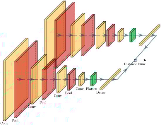
Figure 1.
Siamese network layout.
Table 2.
Siamese network layout.
Similarity scores between two network inputs are calculated based on a distance metric, which needs to be discriminative enough to separate instances of different classes and group together those of the same. The top performing distance functions are Euclidean, Manhattan and Cosine Similarity, given, respectively, by:
where P and Q are n-length vectors with entries and , respectively.
Finally, the decision-making head is a single dense neuron providing a soft-label in the range of 0 to 1, where two identical sequences would result in an output of 0 and highly dissimilar inputs would produce an output close to 1.
The convolutional layers and all but the last dense layer use ‘relu’ as their activation function; the final dense layer uses ‘sigmoid’. The convolution layers are 2D due to the 3D-based input (in our case 65 × 66 STFT image output for each of the three channels). Dropout is used after the first two convolution layers, and max pooling is used to reduce the size of the feature maps. The network has a total of 232,704 trainable parameters.
2.5. Siamese Network Training and Classification
During training, the data are randomly paired up to create a range of data sample pairs and their corresponding labels . The labels are then converted to a similarity score . These are then sent to each branch, updating simultaneously the weights of the two CNN branches so that the loss function is minimised. Once the network has been trained it can then be used to extract feature vectors (rather than similarity scores). Every event encoding can be created and then this can be processed later. This enables a large speed up when testing over an entire dataset as multiple comparisons are avoided.
Specifically, during training, each of the two branches of the network are shown one STFT image, or , with flag 0 if (e.g., both and are earthquakes), or 1 otherwise (e.g., is an earthquake and is a rockfall). The samples, and , are randomly chosen from the training set start pool to keep the classes balanced. In order to balance the number of events across classes, data augmentation is performed by shifting in time class events from the training set in the window to create new events. The output branches create their own encoded vectors (i.e., embeddings) representing the learned features of the input, where the distance between these two vectors determines the similarity score. Given two identical inputs both sides of the network would reach the same encoded vector and therefore the distance between the two would be zero.
Classification is performed on an unseen dataset (test set) by choosing an ‘anchor’ from the training set for each class. In a fully supervised approach, during testing, the anchor would be selected by the user/expert. As noted previously, this is time-consuming and subjective for microseismic signals. Instead, for a semi-supervised approach, we take a data-driven approach to choose an anchor from each class which scores the highest accuracy among its peers. Specifically, we take the highest F1-score within in-training for each class. Note that the F1-score is a standard classification metric, which is the harmonic mean of precision and sensitivity, providing a balanced measure that considers both number of wrongly detected events and the number of missed events—see [10] on how to calculate F1-score for seismic classification. This is important as a label in the training set may be incorrect or the signal-to-noise ratio too low to perform well. It is also possible to provide multiple anchors of the same class to create an aggregate score, which will provide better generalisation (assuming that all of the class anchors are similar) but at the expense of processing time.
A threshold is required to determine which event is considered ‘similar’ enough to be classified/grouped in the same class as the anchor. The best threshold values depend on the distance function used but are generally in the centre of the expected range, e.g., for the 0–1 range.
2.6. Determining Siamese Network Parameters, Distance Function, Decision Threshold and Anchors
In this section, we explain the data-driven approach towards setting the network parameters, effectively choosing the distance function, decision threshold and anchor examplars. This methodology needs to be performed for each dataset to be classified, and thus is important for the purposes of reproducibility.
2.6.1. Network Parameters
To determine optimal network parameters, we tested different learning rates with both statics and decaying rates, with the ADAM optimiser. The learning rate of 0.0005 was found to be optimal for our model and is used in all experiments. The final best-performing model shape is listed in Table 2. Note that initial model configurations with more neurons per layer and the same kernel size resulted in many more trainable parameters but with results which were not significantly different. A dropout of 0.4 was found to be optimal when applied only to the first two layers of the model.
2.6.2. Choice of Distance Function, Decision Threshold and Model Weights
Figure 2 shows that all three distance metrics performed well, in terms of F1-score, on rockfall and earthquake classes. However, as expected, the network struggles with the micro-quake class, which is often labelled with uncertainty in relation to the noise class, as discussed in reference to Table 1. Consistently, the cosine distance function resulted in the best F1-scores across all classes, which is expected since it is less sensitive to magnitude distances, and will be used from now on.
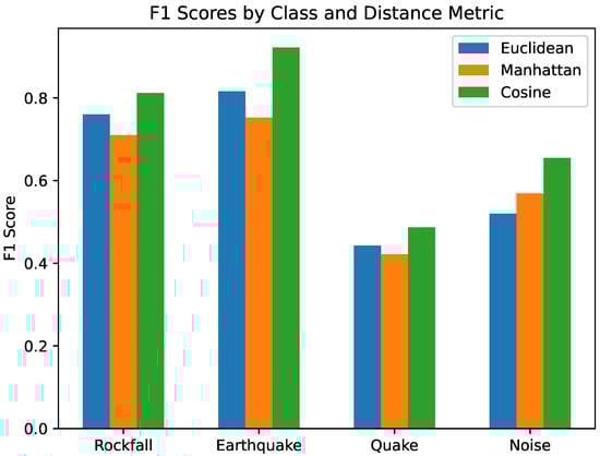
Figure 2.
Performance of different distance functions.
The next step is to determine the optimal decision threshold to decide if a similarity score between a sample and the anchor is high enough for the network to infer that they belong to the same class. We experimentally evaluate the effect of threshold from 0.00 to 1.00 on F1-score. In Figure 3, it can be seen there is little variation across the threshold range, with extremely sharp drop-offs at the two extremes, and the optimal value reached at 0.6. This shows that the network has learned well distinct differences between the classes.
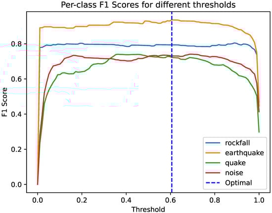
Figure 3.
F1-score per class as threshold is moved. The optimal threshold is highlighted with the dashed line.
To determine optimal model weights, multiple runs were performed for every configuration using sklearns’ StratifiedKFold set to 5 folds. At the start of each fold, the training and validation datasets were created using tensorflow.data.Dataset, which then, were repeated, shuffled (with a set seed) and zipped. Initial training involved all of the training and validation data (70% of all data) being split into 5-folds with 80% being used for training and 20% for validation.
Figure 4 shows the effect that 5-fold validation has on performance. F1-scores for rockfall and earthquake events remain high between folds showing that the data variation between training and validation sets makes little difference to the final performance. Noise performs worse, but has a similar spread in F1-scores. The noise class contains a number of different sub-events which are detected across the training-validation set and therefore it is understandable that changes between folds do not affect performance significantly. Micro-quake events have the greatest spread in performance between folds. Indeed, the micro-quake class has the most varied amount of signal-to-noise ratio and with very short event times; thus, a sub-set of events could be considered more challenging than others as represented by a large spread in F1-scores with the worst being below 0.5. Of the five folds, the best model weights were chosen from fold 3 which had the average F1-scores: rockfall: 0.79; earthquake: 0.94; micro-quake: 0.72; noise: 0.73.
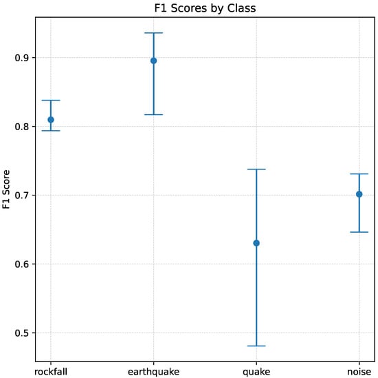
Figure 4.
Best performing model F1-scores over five-fold validation.
2.6.3. Anchor Identification
The Siamese network performs classification by comparing each testing sample with each class representative (i.e., anchor). Cleverly selecting anchors can significantly improve the performance by using only best representative anchors per class from the training set. We demonstrate how to determine the best anchors to use for training in the absence of labels with 100% labelling certainty.
First, the best choice of anchors is obtained using the cosine distance values, illustrated via a heat map in Figure 5. In this heat map, anchor events in darker colours are similar (smaller cosine distance value) whereas lighter (yellow) colours are dissimilar. That is, the smaller the cosine distance, the more similar the event on the vertical-axis is to the class/label on the horizontal axis. The well-defined triangular dark events (equivalent to cosine distance of less than 0.05) on the vertical axis represent events that make good anchors for each of the four class labels on the horizontal axis. Dark vertical or horizontal lines within the lighter portion of the heat map indicate anchor events in each class which have higher similarity, i.e., smaller distance, with events outside their class. These events are outliers, and should not be used as anchors.
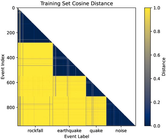
Figure 5.
Identification of events that would make good anchors based on very small cosine distances, indicated by dark well-defined regions for each of the four class labels on the horizontal axis.
Thus, the heat map provides a visual indication of events which would unlikely produce valid results for a given class, and to identify events which may have been wrongly labelled in the catalogue due to expert uncertainty since they are only highly similar to a different class.
Performance of the model was determined using the test set, generating the distance matrix of the encoded test set and comparing against each other to obtain the performance across all ‘anchors’ of each class. We observe that training with only anchors that gave high F1-scores reduced the model performance and, as expected, limiting to only the lowest performing anchors made all classes significantly worse. The best performance trade-off occurred when the middle performing events were chosen from the rockfall and earthquake class and all of the examples from the micro-quake and noise class are considered as training data. The inclusion of all examples from micro-quake highlights the uncertainty around the class with its short duration and for noise the wide range of possible sources means that all should be considered. Removing the best and worst performing anchors from the rockfall and earthquake class did not affect the performance of those classes, but improved the performance of quake and noise. Finally, by picking events with higher F1-scores using the same process as above, the best exemplar anchor candidate per class was chosen. This resulted in improved performance of the model from 0.79 to 0.98 for rockfall, 0.94 to 0.98 earthquake, 0.72 to 0.97 and 0.73 to 0.97 for noise.
We can therefore be confident that the above combination of optimal model weights obtained from 5-fold validation, decision threshold and the optimal anchor per class will result in the best labels when testing on unseen datasets.
3. Results and Discussion
In this section, first we evaluate, through moving window analysis, how effectively features are learnt by the proposed methodology. Secondly, we report the classification performance of the network on the test set using the standard sensitivity and other classification performance metrics, and explain the Siamese network outputs for classification. For benchmarking, we compare the performance with the multi-class CNN classifier of [19] on the same test set, as well as the large pre-trained EQ Transformer model [20] on the same Résif test set looking exclusively at earthquakes to provide a fair comparison.
3.1. Evaluation of Network Learning via Moving Window Analysis
Figure 6 shows the distance across time when running on continuous data: the vertical axis shows the detection for every anchor in the training set, while the horizontal axis shows the time in seconds. The darker the colour, the smaller the distance between the test window and the used anchor. The 10 s window is moved across a 30 s period where the event start time is at 0. We confirm that event detection is in line with the relative duration of events, as per the catalogue reported in Table 1. Indeed, the rockfall can be detected for a large window of time (around 16 s), while micro-quake is very exact at roughly 2.5 s. For earthquakes, the detection time is only around 6 s rather than the catalogued 13 s. This may be due to the network only detecting the initial wave arrivals and losing the signal as the power tails off, and is expected for micro-earthquakes.
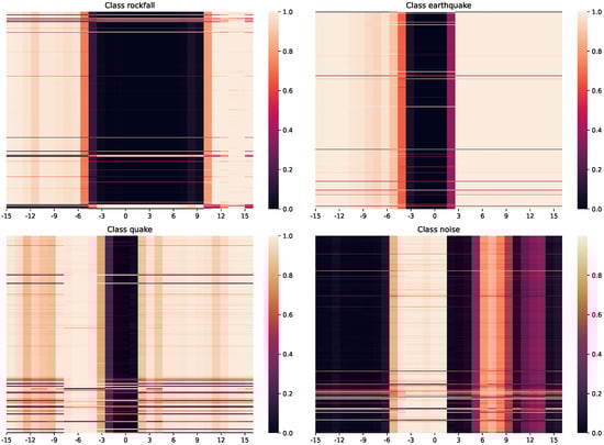
Figure 6.
Moving window for each of the classes when compared against the training anchors. The horizontal axis shows time in seconds, while the vertical axis presents the detection result for every anchor in the training set, i.e., each row represents the result using one anchor. The darker the colour the smaller the cosine distance between the test window and the used anchor.
To demonstrate that the networks learned representative features, we adjusted the time dimension of the STFT image by rolling the input, up to ±4.55 s from their original position as well as up to ±40 Hz in the frequency domain. The heat map in Figure 7 shows expected network behaviour where the distance remains low when the event from the same class is shifted along the time axis, but quickly becomes highly dissimilar when shifted along the frequency axis. As before, darker colours in the figure represent smaller distance and thus higher similarity. On the right-hand-side of the figure, we show a dissimilar comparison where it can be seen that the similarity remains low along the time axis, but on the frequency axis events can quickly appear similar. With rockfalls typically being higher frequency than the earthquakes in the Résif dataset, this is the expected behaviour as rolling the earthquake frequency makes it appear similar to rockfall. This shows that the classification network has learned the frequency domain distinguishing features of each of these two class types and will therefore not match these two inputs when they are within their normal limits.

Figure 7.
A heat map of the cosine distance between two events that belong to the same Rockfall class (left) and different classes (right). Rolling time over continuous recordings (in seconds) (horizontal axis) against frequency (in Hz) (vertical axis) of event against a static test.
3.2. Siamese Network Classification Performance
The testing dataset consists of the (chronologically) last 30% of labels from each class, that is, 117 rockfall events, 119 earthquake events, 74 micro-quake events and 115 noise events. The classification results are shown in Table 3, which shows how many events were correctly matched to the anchor for each class. Of the 117 rockfalls in the test set, 107 rockfall events (true positives) were correctly matched with similarity over the decision threshold, 10 labelled rockfall events were not matched with the anchor (false negatives) and 11 detected events (1 micro-quake, 2 earthquake and 8 noise) were misclassified or incorrectly deemed similar to the rockfall anchor (false positives for rockfall). Relative to class size, micro-quake events perform the worst with 11 micro-to-micro comparisons not resulting in a high similarity score, and hence producing false negatives. There are only a total of 55 misclassifications (dissimilar to the class anchors), the majority being attributed to anthropological noise events, which can take some features of other class anchors due to their variability. For rockfall, earthquake and micro-quake events characterising landslides, there are only 11 misclassifications compared to test size. Adequate anchor choice is therefore critical in being able to correctly detect all of events for each class. Despite imbalance in the number of events in the labelled dataset as shown in Table 1, the results indicate that the imbalance does not impact performance since it is observed that the micro-quake event class, of which there were relatively fewer catalogued during the monitoring period, has no worse performance than other event classes.
Table 3.
Classification performance of test input vs anchor label. In brackets, the number of false negatives is given.
3.3. Explaining Siamese Network Output
The ‘soft label’ distance output from the Siamese network allows us to investigate why certain events may fail to be classified correctly. As Siamese network performance depends on the choice of anchor, to better understand the differences between events within the same class (and therefore which event would make a good anchor), the sensitivity (True Positive Rate (TPR)) of each event index within the test set is plotted in Figure 8. Note that sensitivity measures the proportion of actual positive cases that are correctly identified as positive by the model. A high sensitivity indicates that the model is good at finding most of the positive instances of the class, while a low sensitivity suggests that the model is missing some.
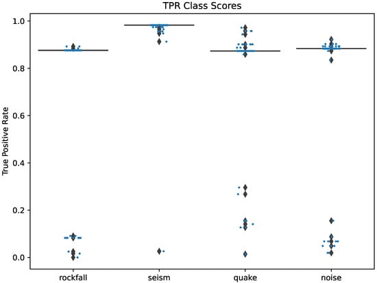
Figure 8.
Class comparison sensitivity. Individual events are plotted with ’.’ to correspond to the box plot diamonds.
Specifically, Figure 8 shows the sensitivity per event compared against all others in its class. A rockfall which is similar to all other rockfalls would have a high sensitivity, and would be a good anchor, while a rockfall which is unique or highly distinct from others would have a great number of misclassifications and therefore a low accuracy and be a bad anchor. It can be seen that earthquake (seism) has only one event which is poor, whereas the other classes have more than one. This is expected since earthquakes have well-defined features and always demonstrate very good performance in the literature. Rockfall has one event which has no true positives, with an event start at 2015-07-07 19:32:49.42.
To illustrate this dissimilarity between this event and other events in the Rockfall class, we show in Figure 9 seismogram images of the rockfall which has no true positives and an alternative event which has a very high sensitivity. Brighter colours represent higher signal amplitude. It can be seen that the low-sensitivity event has no distinct sequence of impacts and has a short initial event with two components around 25 to 35 Hz which look similar to a micro-quake, in comparison to the high-sensitivity event which has more distinct events within the 10 to 20 Hz range which is far more typical for the rockfall events in the dataset; hence, the misclassification. As described in Section 2.1, rockfalls are characterised by distinctive impacts over several seconds, which the model learns, and then it infers during classification that this event is not a rockfall. When compared to the entire testing dataset, we can see in Figure 10 that Event 2015-07-07 19:32:49.42 shares little in common with any of the other rockfalls (according to the Siamese network similarity score) except itself. It does, however, appear to more closely resemble a micro-quake which is understandable given how it appears within the spectrogram in Figure 9. This could be a labelling error, since as reported in the catalogue and as indicated in Table 1, there are labels which are marked as uncertain and there is the possibility that during the labelling process an event was misclassified especially with regards to smaller events such as micro-quakes and rockfalls.
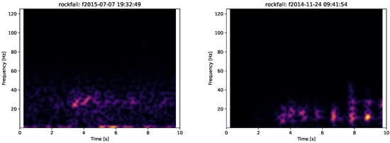
Figure 9.
Comparison between seismograms of two labelled rockfall events: low-sensitivity event at 2015-07-07 19:32:49.42 (left) and high-sensitivity event at 2014-11-24 09:41:54.10 (right). Z component (vertical) is only shown.
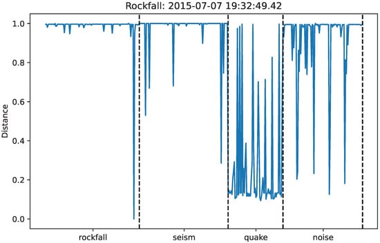
Figure 10.
Rockfall Event Indexed 341 in the dataset: compared against the other testing data, it shows that the network considers it highly different from all other rockfalls (apart from itself, hence the dip at the end of the rockfall labels); it does, however, appear similar to micro-quakes due to its appearance in the spectrogram.
The micro-quake class which contains events which were noted as uncertain in the original catalogue can also be investigated in the same manner. For example, the quake event from 2013 was labelled as a possible rockfall and this can be seen by its elongated spectrum in comparison to the high-sensitivity quake in 2015. Figure 11 is shown below.
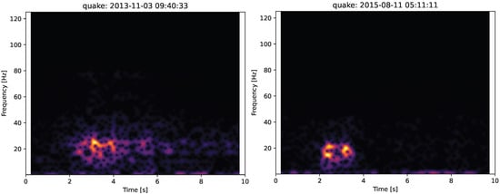
Figure 11.
Comparison between two micro-quake events: low-sensitivity event at 2013-11-03 09:40:33.49 (left) and high-sensitivity event at 2015-08-11 05:11:11.74 (right). Only horizontal component shown.
Thus, the ‘soft label’ from the Siamese network allows us not only to see that the event was misclassified but also helps to explain why it was misclassified. It can be seen that these particular events are considered significantly different from all other events from the same class, which could be due to labelling error (in the quake example) or requires further expert re-evaluation of labels (in the rockfall example).
3.4. Benchmarking Across Other Classifiers
Table 3 shows strong classification performance across all classes, with rockfall prediction being the best and noise being the worst: F1-score rockfall: 0.90; earthquake: 0.97; micro-quake: 0.88; noise: 0.84. This is expected since noise can be from any number of sources and has no predefined frequency bands. This is in line with the performance of [19], where F1-score for rockfalls, earthquakes, micro-quakes and noise for the CNN model for STFT inputs were 0.9, 0.97 and 0.88, 0.86, respectively. This confirms our earlier hypothesis that Siamese networks require less training data (Rockfall: 241 to 126 events; Earthquake: 233 to 104; Quake: 141 to 131; Noise 210 to 190), without compromising on performance. Furthermore, transferability and generalisability of the classification studies in this dataset have been shown in [10,19] for recordings from Austria and Greece, respectively. The classification results obtained by our experiments are in line with these studies. The same Siamese-based trained network was used to identify micro-seismic events on the Hollin Hill Landslide Observatory [14], which is comparable to a number of other sites within the European Alps in terms of rheological properties of clayey soils in flow-like landslides. In summary, classification results from [14,19], using the same dataset for training but testing on other datasets, demonstrate the applicability of the proposed methodology across geologically distinct sites in different countries.
We also benchmark earthquake event performance against the state-of-the-art EQTransformer (EQT) [20], a binary classifier developed for testing earthquake events. EQT has two publicly available models: a ‘regular’ (described in the original paper [20]) and a ‘conservative’ model (available on GitHub). The regular model is highly effective at detecting earthquake events; however, its higher sensitivity makes it prone to detecting similar non-seismic events, leading to high numbers of false positives. The conservative model, on the other hand, produces significantly less false positives but at the expense of missing many true events. Both models have manually tunable threshold values, both for P and S wave picking, as well as detection, to help control false positives.
Samples are only considered as events if EQT can detect them across multiple stations (assuming multiple station inputs). We use the seismograms from station SZC of the test events from Table 1 and for each model adjust the EQT detection threshold (using values 0.9, 0.8, 0.1) while keeping the default P and S thresholds. Since EQT is a binary classifier, it will detect only earthquakes. Therefore, correct detection of earthquake events is treated as true positives, and misclassification of micro-quake and rockfall events as earthquake events is treated as false positives during our metric calculations.
As expected, Table 4 shows that the regular model has a higher sensitivity and lower precision compared to the conservative model, with increasing sensitivity and decreasing precision as the detection threshold decreases. Note that the conservative model with a threshold 0.1 is most similar to the regular model at 0.9. Comparing with the Earthquake performance of the Siamese network on the same test set in Table 3, the performance across the Résif earthquakes is significantly poorer for EQT than would be expected with just more than half the earthquakes detected with the regular model and only half detected with the conservative model. This can be explained by the low magnitudes of the events, M < 1, for earthquakes present within the Résif dataset [16].
Table 4.
EQT performance (excluding noise).
4. Conclusions
This paper proposes an unbounded method of microseismic event detection and classification on continuous data using a Siamese network, based on a data-driven design strategy for the training of the Siamese network to determine best decision thresholds, model weights and anchor choice that will result in an optimal model. We demonstrate the performance of the proposed methodology on the challenging Résif dataset, which comprises four classes of events with heterogeneous signal characteristics within a class. The key findings of the study can be summarised as follows. The proposed semi-supervised methodology shows that limiting training data based on performance of given anchors informs selection of an exemplar anchor per class to be taken forward to unseen testing data. We demonstrate that while operating as a classifier with known event types, the performance is in line with other supervised models but requires less training examples. Indeed, only 126 rockfall events, 104 earthquake events, 131 micro-quake events and 190 noise events were needed for training compared to significantly more events needed for benchmarked supervised classification approaches. This means that labelling can be automated with high confidence with a known exemplar anchor, which could be taken from a known external dataset or via manual identification at the site in question, to ensure high similarity to local conditions. Additionally, via the Siamese ‘soft labelling’, we show how it is possible to explain why certain events are missed or misclassified. As shown in [14], the proposed methodology could be applied for fast categorisation of datasets with minimal ground truth available.
Future work would look to make use of clustering methods on the encoded seismic data to label unknown events via grouping. Furthermore, a good direction for future work is to optimise data-acquisition methods in conjunction with classification.
Author Contributions
D.M.: Conceptualisation, Methodology, Software, Validation, Formal analysis, Investigation, Writing—original draft, Writing—review and editing, Visualisation. L.S.: Conceptualisation, Formal analysis, Investigation, Writing—review and editing, Supervision, Project administration, Funding acquisition. V.S.: Conceptualisation, Validation, Formal analysis, Investigation, Writing—review and editing, Supervision, Funding acquisition. All authors have read and agreed to the published version of the manuscript.
Funding
This work was supported by the EPSRC under the New Horizons programme under grant agreement No. EP/X01777X/1.
Data Availability Statement
The dataset used in this paper is the Résif dataset available at [9].
Acknowledgments
We thank F. Provost for providing a catalogue of labelled events used in this paper.
Conflicts of Interest
The authors declare that they have no known competing financial interests or personal relationships that could have appeared to influence the work reported in this paper.
References
- Huang, W.; Zhang, W.; Li, L.; Zhang, H.; Li, F. Review on Low-noise Broadband Fiber Optic Seismic Sensor and its Applications. J. Light. Technol. 2023, 41, 4153–4163. [Google Scholar] [CrossRef]
- Zhu, C.; Wang, C.; Zhang, B.; Qin, X.; Shan, X. Differential Interferometric Synthetic Aperture Radar data for more accurate earthquake catalogs. Remote Sens. Environ. 2021, 266, 112690. [Google Scholar] [CrossRef]
- Zhao, S.; McClusky, S.; Cummins, P.R.; Miller, M.S. Co-seismic and post-seismic deformation associated with the 2018 Lombok, Indonesia, earthquake sequence, inferred from InSAR and seismic data analysis. Remote Sens. Environ. 2024, 304, 114063. [Google Scholar] [CrossRef]
- Mao, S.; Lecointre, A.; van der Hilst, R.D.; Campillo, M. Space-time monitoring of groundwater fluctuations with passive seismic interferometry. Nat. Commun. 2022, 13, 4643. [Google Scholar] [CrossRef]
- Jousset, P.; Currenti, G.; Schwarz, B.; Chalari, A.; Tilmann, F.; Reinsch, T.; Zuccarello, L.; Privitera, E.; Krawczyk, C.M. Fibre optic distributed acoustic sensing of volcanic events. Nat. Commun. 2022, 13, 1753. [Google Scholar] [CrossRef]
- Spica, Z.J.; Ajo-Franklin, J.; Beroza, G.C.; Biondi, B.; Cheng, F.; Gaite, B.; Luo, B.; Martin, E.; Shen, J.; Thurber, C.; et al. PubDAS: A PUBlic Distributed Acoustic Sensing Datasets Repository for Geosciences. Seismol. Res. Lett. 2023, 94, 983–998. [Google Scholar] [CrossRef]
- Vasconez, F.J.; Silvana, H.; Jean, B.; Stephen, H.; Benjamin, B.; Diego, C.; Sébastien, V.; Patricio, R.; Santiago, A.; Céline, L.; et al. Linking ground-based data and satellite monitoring to understand the last two decades of eruptive activity at Sangay volcano, Ecuador. Bull. Volcanol. 2022, 84, 49. [Google Scholar] [CrossRef]
- Lu, P.; Qin, Y.; Li, Z.; Mondini, A.C.; Casagli, N. Landslide mapping from multi-sensor data through improved change detection-based Markov random field. Remote Sens. Environ. 2019, 231, 111235. [Google Scholar] [CrossRef]
- French Landslide Observatory Seismological Datacenter RESIF. Observatoire Multi-Disciplinaire des Instabilites de Versants (OMIV). 2023. Available online: https://seismology.resif.fr/networks/#/MT (accessed on 31 July 2025).
- Li, J.; Stankovic, L.; Pytharouli, S.; Stankovic, V. Automated Platform for Microseismic Signal Analysis: Denoising, Detection, and Classification in Slope Stability Studies. IEEE Trans. Geosci. Remote Sens. 2020, 59, 7996–8006. [Google Scholar] [CrossRef]
- Jiang, J.; Murray, D.; Stankovic, V.; Stankovic, L.; Hibert, C.; Pytharouli, S.; Malet, J.P. A human-on-the-loop approach for labelling seismic recordings from landslide site via a multi-class deep-learning based classification model. Sci. Remote Sens. 2025, 11, 100189. [Google Scholar] [CrossRef]
- Saha, S.; Bera, B. Rainfall threshold for prediction of shallow landslides in the Garhwal Himalaya, India. Geosyst. Geoenviron. 2024, 3, 100285. [Google Scholar] [CrossRef]
- Li, J.; Li, B.; He, K.; Gao, Y.; Wan, J.; Wu, W.; Zhang, H. Failure Mechanism Analysis of Mining-Induced Landslide Based on Geophysical Investigation and Numerical Modelling Using Distinct Element Method. Remote Sens. 2022, 14, 6071. [Google Scholar] [CrossRef]
- Murray, D.; Stankovic, L.; Stankovic, V.; Pytharouli, S.; White, A.; Dashwood, B.; Chambers, J. Characterisation of precursory seismic activity towards early warning of landslides via semi-supervised learning. Sci. Rep. 2025, 15, 1026. [Google Scholar] [CrossRef] [PubMed]
- Boginskaya, N.V.; Kostylev, D.V. Change in the Level of Microseismic Noise During the COVID-19 Pandemic in the Russian Far East. Pure Appl. Geophys. 2022, 179, 4207–4219. [Google Scholar] [CrossRef] [PubMed]
- Provost, F.; Hibert, C.; Malet, J.P. Automatic classification of endogenous landslide seismicity using the Random Forest supervised classifier. Geophys. Res. Lett. 2017, 44, 113–120. [Google Scholar] [CrossRef]
- Hibert, C.; Provost, F.; Malet, J.P.; Maggi, A.; Stumpf, A.; Ferrazzini, V. Automatic identification of rockfalls and volcano-tectonic earthquakes at the Piton de la Fournaise volcano using a Random Forest algorithm. J. Volcanol. Geotherm. Res. 2017, 340, 130–142. [Google Scholar] [CrossRef]
- Wu, Y.; Lin, Y.; Zhou, Z.; Bolton, D.C.; Liu, J.; Johnson, P. DeepDetect: A Cascaded Region-Based Densely Connected Network for Seismic Event Detection. IEEE Trans. Geosci. Remote Sens. 2019, 57, 62–75. [Google Scholar] [CrossRef]
- Jiang, J.; Stankovic, V.; Stankovic, L.; Parastatidis, E.; Pytharouli, S. Microseismic Event Classification with Time-, Frequency-, and Wavelet-Domain Convolutional Neural Networks. IEEE Trans. Geosci. Remote Sens. 2023, 61, 5906414. [Google Scholar] [CrossRef]
- Mousavi, S.M.; Ellsworth, W.L.; Zhu, W.; Chuang, L.Y.; Beroza, G.C. Earthquake transformer—an attentive deep-learning model for simultaneous earthquake detection and phase picking. Nat. Commun. 2020, 11, 3952. [Google Scholar] [CrossRef]
- Trani, L.; Pagani, G.A.; Zanetti, J.P.P.; Chapeland, C.; Evers, L. DeepQuake—An application of CNN for seismo-acoustic event classification in The Netherlands. Comput. Geosci. 2022, 159, 104980. [Google Scholar] [CrossRef]
- Xiao, Z.; Wang, J.; Liu, C.; Li, J.; Zhao, L.; Yao, Z. Siamese Earthquake Transformer: A Pair-Input Deep-Learning Model for Earthquake Detection and Phase Picking on a Seismic Array. J. Geophys. Res. Solid Earth 2021, 126, e2020JB021444. [Google Scholar] [CrossRef]
- Zhu, W.; Beroza, G.C. PhaseNet: A deep-neural-network-based seismic arrival-time picking method. Geophys. J. Int. 2018, 216, 261–273. [Google Scholar] [CrossRef]
- Murray, D.; Stankovic, L.; Stankovic, V. Siamese unsupervised clustering for removing uncertainty in microseismic signal labelling. In Proceedings of the 2024 IEEE International Geoscience and Remote Sensing Symposium, IGARSS 2024, Athens, Greece, 7–12 July 2024; pp. 8816–8820. [Google Scholar] [CrossRef]
- Feng, L.; Pazzi, V.; Intrieri, E.; Gracchi, T.; Gigli, G. Rockfall seismic features analysis based on in situ tests: Frequency, amplitude, and duration. J. Mt. Sci. 2019, 16, 955–970. [Google Scholar] [CrossRef]
- Anikiev, D.; Birnie, C.; bin Waheed, U.; Alkhalifah, T.; Gu, C.; Verschuur, D.J.; Eisner, L. Machine learning in microseismic monitoring. Earth-Sci. Rev. 2023, 239, 104371. [Google Scholar] [CrossRef]
- Grubas, S.; Yaskevich, S.; Duchkov, A. Localization of microseismic events using the physics-informed neural-network for traveltime computation. In Proceedings of the 82nd EAGE Annual Conference & Exhibition, Amsterdam, The Netherlands, 18–21 October 2021; Volume 2021, pp. 1–5. [Google Scholar] [CrossRef]
- Giudicepietro, F.; Esposito, A.M.; Spina, L.; Cannata, A.; Morgavi, D.; Layer, L.; Macedonio, G. Clustering of Experimental Seismo-Acoustic Events Using Self-Organizing Map (SOM). Front. Earth Sci. 2021, 8, 581742. [Google Scholar] [CrossRef]
- Liao, X.; Cao, J.; Hu, J.; You, J.; Jiang, X.; Liu, Z. First Arrival Time Identification Using Transfer Learning with Continuous Wavelet Transform Feature Images. IEEE Geosci. Remote Sens. Lett. 2020, 17, 2002–2006. [Google Scholar] [CrossRef]
- Zhang, G.; Lin, C.; Chen, Y. Convolutional neural networks for microseismic waveform classification and arrival picking. Geophysics 2020, 85, WA227–WA240. [Google Scholar] [CrossRef]
- Iqbal, N. DeepSeg: Deep Segmental Denoising Neural Network for Seismic Data. IEEE Trans. Neural Networks Learn. Syst. 2022, 34, 3397–3404. [Google Scholar] [CrossRef]
- Liao, W.Y.; Lee, E.J.; Wang, C.C.; Chen, P.; Provost, F.; Hiber, C.; Malet, J.P.; Chu, C.R.; Lin, G.W. RockNet: Rockfall and earthquake detection and association via multitask learning and transfe learning. Authorea 2022. [Google Scholar] [CrossRef]
- Müller, T.; Pérez-Torró, G.; Franco-Salvador, M. Few-Shot Learning with Siamese Networks and Label Tuning. In Proceedings of the 60th Annual Meeting of the Association for Computational Linguistics (Volume 1: Long Papers), Dublin, Ireland, 22–27 May 2022; pp. 8532–8545. [Google Scholar] [CrossRef]
- Heydari, S.S.; Mountrakis, G. Effect of classifier selection, reference sample size, reference class distribution and scene heterogeneity in per-pixel classification accuracy using 26 Landsat sites. Remote Sens. Environ. 2018, 204, 648–658. [Google Scholar] [CrossRef]
- Cao, Y.; Huang, X.; Weng, Q. A multi-scale weakly supervised learning method with adaptive online noise correction for high-resolution change detection of built-up areas. Remote Sens. Environ. 2023, 297, 113779. [Google Scholar] [CrossRef]
- Hou, L.; Jin, X.; Zhao, Z. Time Series Similarity Measure via Siamese Convolutional Neural Network. In Proceedings of the 2019 12th International Congress on Image and Signal Processing, BioMedical Engineering and Informatics (CISP-BMEI), Suzhou, China, 19–21 October 2019; pp. 1–6. [Google Scholar] [CrossRef]
- Awal, A.M.; Ghanmi, N.; Sicre, R.; Furon, T. Complex Document Classification and Localization Application on Identity Document Images. In Proceedings of the 2017 14th IAPR International Conference on Document Analysis and Recognition (ICDAR), Kyoto, Japan, 9–15 November 2017; Volume 1, pp. 426–431. [Google Scholar] [CrossRef]
- Ruan, G.; Kirschen, D.S.; Zhong, H.; Xia, Q.; Kang, C. Estimating Demand Flexibility Using Siamese LSTM Neural Networks. IEEE Trans. Power Syst. 2022, 37, 2360–2370. [Google Scholar] [CrossRef]
- Li, Y.; Chen, C.L.P.; Zhang, T. A Survey on Siamese Network: Methodologies, Applications, and Opportunities. IEEE Trans. Artif. Intell. 2022, 3, 994–1014. [Google Scholar] [CrossRef]
- Sameer, V.U.; Naskar, R. Deep siamese network for limited labels classification in source camera identification. Multimed. Tools Appl. 2020, 79, 28079–28104. [Google Scholar] [CrossRef]
- Liu, Y.; Ding, L.; Chen, C.; Liu, Y. Similarity-Based Unsupervised Deep Transfer Learning for Remote Sensing Image Retrieval. IEEE Trans. Geosci. Remote Sens. 2020, 58, 7872–7889. [Google Scholar] [CrossRef]
Disclaimer/Publisher’s Note: The statements, opinions and data contained in all publications are solely those of the individual author(s) and contributor(s) and not of MDPI and/or the editor(s). MDPI and/or the editor(s) disclaim responsibility for any injury to people or property resulting from any ideas, methods, instructions or products referred to in the content. |
© 2025 by the authors. Licensee MDPI, Basel, Switzerland. This article is an open access article distributed under the terms and conditions of the Creative Commons Attribution (CC BY) license (https://creativecommons.org/licenses/by/4.0/).