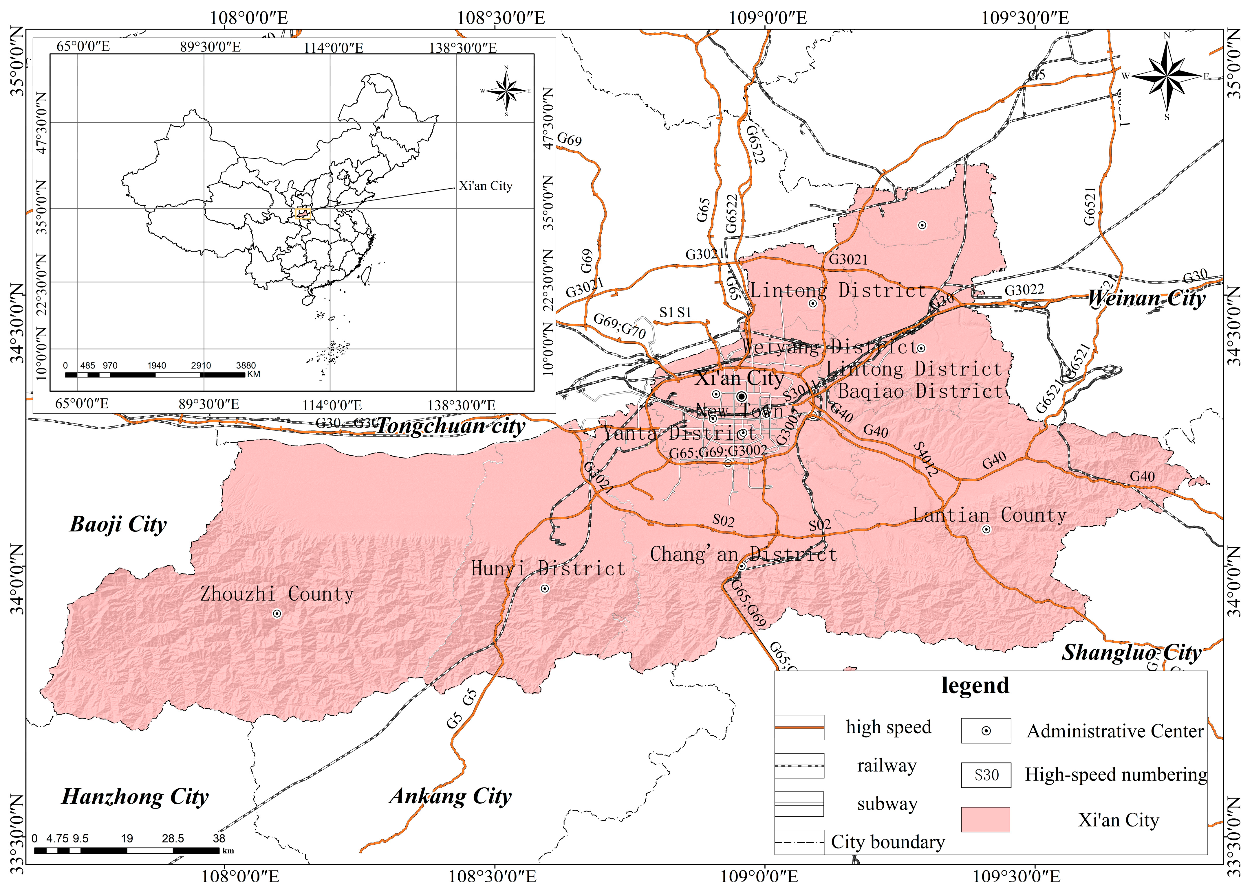
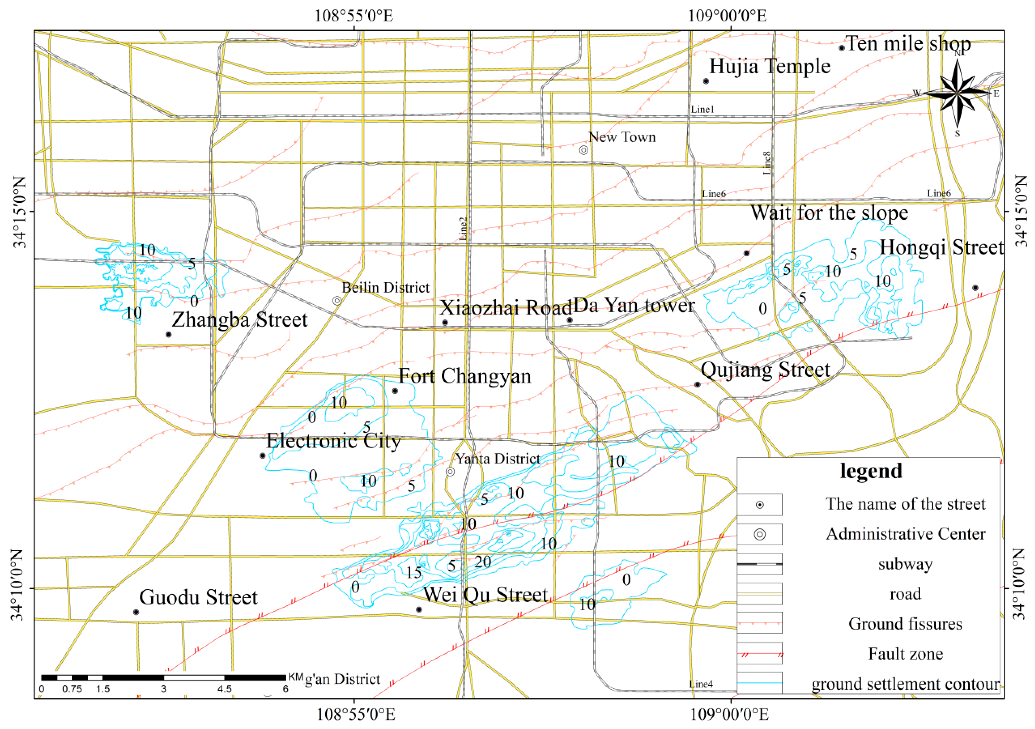
Article

Geological Hazard Susceptibility Assessment Based on the Combined Weighting Method: A Case Study of Xi’an City, China

1
School of Geological Engineering and Geomatics, Chang’an University, Xi’an 710061, China
2
Machinery Industry Survey, Design and Research Institute Co., Ltd., Xi’an 710021, China
3
CCCC First Highway Survey, Design and Research Institute Co., Ltd., Xi’an 710075, China
*
Author to whom correspondence should be addressed.
Geosciences 2025, 15(8), 290; https://doi.org/10.3390/geosciences15080290 (registering DOI)
Submission received: 13 June 2025 / Revised: 23 July 2025 / Accepted: 28 July 2025 / Published: 1 August 2025

Abstract

Xi’an, China, has a complex geological environment, with geological hazards seriously hindering urban development and safety. This study analyzed the conditions leading to disaster formation and screened 12 evaluation factors (e.g., slope and slope direction) using Spearman’s correlation. Furthermore, it also introduced an innovative combined weighting method, integrating subjective weights from the hierarchical analysis method and objective weights from the entropy method, as well as an information value model for susceptibility assessment. The main results are as follows: (1) There are 787 hazard points—landslides/collapses are concentrated in loess areas and Qinling foothills, while subsidence/fissures are concentrated in plains. (2) The combined weighting method effectively overcame the limitations of single methods. (3) Validation using hazard density and ROC curves showed that the combined weighting information value model achieved the highest accuracy (AUC = 0.872). (4) The model was applied to classify the disaster susceptibility of Xi’an into high (12.31%), medium (18.68%), low (7.88%), and non-susceptible (61.14%) zones. The results are consistent with the actual distribution of disasters, thus providing a scientific basis for disaster prevention.

1. Introduction

Geological hazards refer to disasters that endanger public life and property safety caused by natural factors or human activities, characterized by suddenness, persistence, and clustering. These include landslides, collapses, debris flows, ground collapse, ground fissures, ground subsidence, and other disasters directly related to natural geological influences [1,2]. In recent years, with accelerating urbanization processes and intensifying human engineering activities, the frequency of geological hazards and the resulting losses have demonstrated an upward trend; this is particularly the case in areas with complex geological conditions and dense populations, where geological hazards have become important factors threatening regional socioeconomic sustainable development [3,4]. As a significant city in Northwest China, Xi’an City is located in the transitional zone between the Guanzhong Plain and the Qinling Mountains. This area is characterized by complex geological structures, complete stratigraphic development, significant topographic relief, pronounced seasonal rainfall patterns, and frequent human engineering activities. Various geological hazards frequently occur, posing a serious threat to the lives and property of local residents and the city’s healthy development. Therefore, conducting geological hazard susceptibility assessment research in Xi’an City and scientifically delineating geological hazard-prone areas holds significant theoretical and practical significance for guiding geological hazard prevention and control work and ensuring regional safety.
Geological hazard susceptibility assessment refers to the prediction and evaluation of the probability of geological hazards occurring within specific regions and is an important component of geological hazard risk assessment [5,6]. Currently, geological hazard susceptibility assessment methods are primarily divided into two major categories: qualitative and quantitative assessment. Qualitative assessments mainly include expert experience methods, the analytic hierarchy process, and fuzzy comprehensive evaluation methods which, although simple to operate, are relatively subjective and yield evaluation results with relatively low accuracy and reliability [7,8]. With the development of 3S and computer technologies, quantitative assessment methods have been widely applied, primarily encompassing mathematical statistical models and machine learning models [9,10]. Mathematical statistical models such as certainty factor models, information value models, and logistic regression models can objectively reflect the relationships between assessment factors and geological hazards, but they face difficulties in handling complex, nonlinear relationships [11,12]. In recent years, machine learning models such as random forest, support vector machine, XGBoost, and artificial neural networks have been widely applied in geological hazard susceptibility assessments due to their capability to process high-dimensional data and complex nonlinear relationships [13,14,15,16,17]. However, single models often possess limitations and cannot comprehensively reflect the complex causative mechanisms of geological hazards. Multi-model coupling and ensemble learning methods have attracted researchers’ attention because they can integrate the advantages of various models [18,19,20].
In geological hazard susceptibility assessment, it is critical to determine evaluation indicator weights, since they directly influence the accuracy of assessment results. Weight determination methods are primarily classified into three categories: subjective, objective, and combined weighting methods [21,22]. Subjective weighting methods, such as the analytic hierarchy process and the Delphi method, rely on expert experience and subjective judgment, possessing clear physical significance, but often exhibit certain biases due to the limitations of individual subjective cognition [23]. Objective weighting methods, such as the entropy weight method, coefficient of variation method, and principal component analysis, rely entirely on data information and can avoid interference from human factors; however, they may overlook the actual importance of indicators [24,25]. Combined weighting methods integrate the advantages of both subjective and objective weighting approaches, enabling more comprehensive and reasonable determination of evaluation indicator weights and enhancing the scientific validity and reliability of assessment results [26,27,28]. Huang, Siyi [3] obtained good results in the spatial prediction of the geohazard vulnerability of mountain road networks using machine learning algorithms. Cheng, K et al. [29] performed a cloud modeling-based analysis of spatial variation in water resources’ carrying capacity, and the identification of influencing factors showed that the combined assignment method was effective.
International scholars have also conducted extensive research in this field. Guzzetti et al. [30] conducted multi-scale landslide hazard assessment research in Central Italy, systematically summarizing the main technical methods at that time and laying an important foundation for the development of this field. Steger et al. [31] conducted research in European regions and found that the incompleteness of landslide samples significantly affects the validation results of statistical models and geomorphological rationality. They proposed systematic methods for improving landslide susceptibility mapping accuracy. Yalcin et al. [32] conducted a comparative study of GIS-based landslide susceptibility assessment methods in the Trabzon region of Turkey, systematically comparing the evaluation effects of multiple methods, including the frequency ratio, analytic hierarchy process, bivariate statistics, and logistic regression. Pradhan et al. [33] compared the application effects of artificial neural networks, the frequency ratio, and bivariate logistic regression methods in landslide susceptibility assessment, demonstrating the advantages of machine learning approaches. Ballabio et al. [34] conducted in-depth research specifically on the application of support vector machines in landslide susceptibility mapping and proposed effective methods for SVM model parameter optimization. Goetz et al. [35] conducted comparative studies of various machine learning and statistical prediction techniques, systematically evaluating the performance differences in different models in landslide susceptibility modeling. Brenning [36] conducted comprehensive comparisons of various spatial prediction models, which hold important value in terms of theoretical foundations. Raspini et al. [37] developed continuous, semi-automatic surface deformation monitoring methods based on Sentinel-1 satellite data, providing new technical support for landslide susceptibility assessment. Reichenbach et al. [38] conducted a comprehensive review of statistics-based landslide susceptibility models, systematically comparing the performance differences between traditional statistical methods and modern machine learning approaches.
As a region with frequent geological hazards, Xi’an City exhibits diverse geological hazard types, a widespread distribution, and complex causative mechanisms, making traditional single-weight determination methods inadequate for accurately reflecting the contribution of various influencing factors to geological hazard susceptibility. Based on the geological environmental conditions and geological hazard characteristics of Xi’an City, this study comprehensively analyzed the characteristics and development patterns of geological hazards to select appropriate evaluation indicators.

2. Study Area Overview

2.1. Physical Geography

Xi’an City is located south–centrally in Shaanxi Province, spanning 107°40′–109°49′ E longitude and 33°42′–34°45′ N latitude. The city is bounded by the Bashanyuan Mountains to the east, extends to the Taibai Mountain area to the west, reaches the main ridge of the Qinling Mountains to the south, and borders the Wei River to the north. The city measures 204 km from east to west and 116 km from north to south, with a total area of 10,588.9 km2 (Figure 1).
Xi’an City exhibits a warm temperate semi-humid continental monsoon climate, characterized by complex and variable regional topography and a pronounced vertical climate distribution with outstanding regional differences. From north to south, with increasing elevation, temperature decreases while precipitation increases [39] (Figure 2). The annual average precipitation is 599.42 mm, with a maximum of 903.2 mm (1983) and a minimum of 312.2 mm (1995). Precipitation is predominantly concentrated during July–September, accounting for approximately 49.23% of the annual rainfall. Xi’an City possesses abundant river development, primarily including the Wei River, Ba River, Chan River, Feng River, Hao River, Lao River, Hei River, and Jing River, with the Wei River being the largest, spanning approximately 150 km in the area.

2.2. Topography and Geomorphology

The study area exhibits complex and diverse topography and geomorphology, generally demonstrating a pattern of high elevation in the south and low elevation in the north, as well as high elevation in the east and low elevation in the west. The main geomorphological types include alluvial and alluvial–pluvial plain areas (accounting for approximately 30.11% of the total area), piedmont pluvial plain areas (approximately 8.25%), loess landform areas (approximately 12.08%), and mountainous regions (approximately 49.56%). The mountainous regions can be roughly divided into low mountain regions (with average elevations of approximately 500–1000 m), middle mountain regions (with average elevations of approximately 1000–3500 m), and high mountain regions (with average elevations of approximately 3500–3767.2 m), with the middle mountain areas covering the largest area, forming unique regional geomorphological landscape characteristics (Figure 3).

2.3. Stratigraphy and Lithology

Xi’an City possesses complex stratigraphic conditions with diverse lithologies. Strata of all geological ages are exposed within the area, including the Neoarchean Taihua Group; Paleoproterozoic Tietinggou Formation; Neoproterozoic Xiong’er Group; Lower Paleozoic Danfeng Group; Upper Paleozoic Devonian, Carboniferous, and Permian systems; Mesozoic Triassic and Cretaceous systems; and Cenozoic Paleogene, Neogene, and Quaternary systems. Among these, Quaternary deposits are widely distributed, primarily comprising glaciofluvial sedimentary layers, aeolian layers, pluvial layers, and alluvial-pluvial layers (Table 1).

2.4. Geological Structure

Xi’an City exhibits well-developed geological structures with numerous interlaced active faults. The main fault structures include the Kouzhen–Guanshan Fault (F1), Jingyang–Weinan Fault (F2), North Bank of Wei River Fault (F3), Lishan Piedmont Fault (F4), Lintong–Chang’an Fault (F5), Chan River Fault (F6), Zao River Fault (F7), Hao River Fault (F8), Feng River Fault (F9), Qishan–Mazhao Fault (F10), Yuxia–Tielüzi Fault (F11), Western Huashan Fault (F12), and Qinling Piedmont Fault (F13) (Figure 4). Due to the influence of neotectonic movements, Xi’an City is situated within a northeast–southwest compressive stress field, with the Wei River Basin exhibiting horizontal extensional conditions, forming a structural pattern characterized by basin subsidence and Qinling mountainous area uplift.

2.5. Engineering Geological Properties and Characteristics of Rock and Soil Masses

The soil masses in Xi’an City primarily comprise loose soils of Quaternary alluvial, pluvial, and aeolian origins, which can be classified into two major categories: general soils (sandy soil, gravel soil, and cohesive soil) and special soils (loess, loess-like soil, and artificial fill). The exposed rock types are diverse, primarily comprising intrusive rocks (such as granite), metamorphic rocks (such as phyllite, quartzite, and gneiss), and sedimentary rocks (such as mudstone, sandstone, and conglomerate). Based on engineering geological characteristics, the area can be divided into soil mass engineering geological zones (I) and rock mass engineering geological zones (II), with the soil mass engineering geological zone subdivided into five subzones and the rock mass engineering geological zone subdivided into three subzones, each possessing distinct engineering geological characteristics (Figure 5).

2.6. Hydrogeological Conditions

The study area is rich in groundwater resources, which have promoted the vigorous development of industrial and agricultural production and provided a convenient domestic water supply for urban and rural residents. The conditions that influence the formation of groundwater are complex and depend on various natural factors, including geomorphological types, stratigraphic structures, and precipitation patterns. Different natural conditions result in significant variations in the spatial and temporal distribution of groundwater, thus generating complex hydrological conditions and groundwater types. The types of groundwater mainly include porous water in unconsolidated rocks, pore-fissure water, and bedrock fissure water. The recharge sources of groundwater mainly include precipitation, river runoff, lateral infiltration, and irrigation. The discharge patterns mainly include vertical evaporation discharge, horizontal discharge to rivers, and discharge in the form of springs.

3. Methods

3.1. Data Sources and Preprocessing

The DEM digital elevation data for the study area comprises raster data units with a resolution of 12.5 m × 12.5 m, sourced from the Geospatial Data Cloud (http://www.gscloud.cn/) accessed on 20 July 2024, totaling 64,669,726 evaluation units. Administrative division vector data were obtained from the National Fundamental Geographic Information System (http://snsm.mnr.gov.cn/) and cross-referenced with the latest administrative boundary data from the Xi’an Geological Environment Monitoring Station. Data on topography and geomorphology, river systems, and road distribution were all based on the latest atlases published by Xi’an Map Publishing House. Stratigraphic and lithological data were derived from “Regional Geology of China: Shaanxi Volume.” Geological structural data combined information from “Regional Geology of China: Shaanxi Volume” and the latest materials from the Shaanxi Earthquake Administration. Rock and soil mass classification data were based on “Research on Geology, Geomorphology, and Regional Engineering Geological Conditions of Greater Xi’an” and detailed geological survey materials from various districts and counties. Precipitation data were sourced from the National Meteorological Information Center (http://data.cma.cn/), and monitoring data stemmed from Xi’an Meteorological Bureau rainfall stations. Ground motion parameters were based on the “Seismic Ground Motion Parameters Zonation Map of China” (GB18306-2015) [40] (http://www.gb18306.net/), and the geographic coordinate system adopted in the map is GCS_WGS_1984, using the WGS_1984_World_Mercator projection coordinate system.
Data were sourced from the 2005 geological hazard investigation and zoning reports of various districts and counties in Xi’an City and the 2013 detailed geological hazard investigation report of Lantian County. The 2016 detailed geological hazard investigation reports of Lintong District, Baqiao District, Chang’an District, and Zhouzhi County were combined with geological hazard hidden danger point data from the comprehensive geological hazard system implementation plans of the Xi’an Natural Resources Bureau from 2016 to 2021. A total of 787 geological hazard hidden danger points were statistically compiled (Figure 6), encompassing two major categories: sudden-onset geological hazards and progressive geological hazards.

Types and Development Characteristics of Geological Hazards

(1) Characteristics of Sudden-Onset Geological Hazards
Sudden-onset geological hazards in Xi’an City primarily include landslides, collapses, debris flows, and ground collapse. Their basic characteristics are detailed in Table 2.
(2) Characteristics of Progressive Geological Hazards
Progressive geological hazards primarily include ground fissures and ground subsidence. Ground fissures, in addition to the 12 ground fissures in the urban area, include 10 ground fissures in suburban areas, mainly distributed in Baqiao District (4 fissures), Chang’an District (3 fissures), Yanliang District (2 fissures), and Zhouzhi County (1 fissure). Urban ground fissures are primarily distributed as 12 approximately northeast-trending fissures on the northwest side of the Lintong–Chang’an Fault, covering an area of approximately 250 km2 with a total length of approximately 160 km, of which over 70 km are exposed at the surface, with the longest single exposed fissure measuring approximately 13 km. Ground subsidence mainly appeared in the late 1950s, with five subsidence areas within the region: the Yuhuazhai subsidence area, Electronics City subsidence area, Dongsanyao Village subsidence area, Xidengjiaozhao subsidence area, and Chang’an District Aerospace Industrial Park subsidence area. The total area with deformation rates exceeding 10 mm/a is approximately 28 km2, with maximum subsidence rates of approximately 60 mm/a (see Figure 7 and Figure 8). Geological hazards demonstrate significant differences in distribution among different geomorphological units, with landslides, collapses, and debris flows mainly distributed in loess landform areas and mountainous regions, while ground collapse and ground fissures are primarily distributed in alluvial and alluvial–pluvial plains and loess landform areas.
In the data preprocessing stage, coordinate system unification and geometric correction were first performed on all spatial data. Using the densification function in ArcGIS, 12 ground fissures were converted into 13,881 equivalent points at 50 m intervals, and the contour lines of 5 ground subsidence areas were converted into 12,440 equivalent points at 20 m intervals, with corresponding weight values assigned through kernel density analysis. All raster data were uniformly resampled to a 12.5 m resolution, and quality checks and outlier processing were conducted to establish a data foundation for subsequent multi-factor overlay analysis and model construction.

3.2. Construction of Evaluation Index System

Based on previous research, 13 candidate evaluation indicators were initially selected, including topographic and geomorphological indicators (elevation, slope, aspect, relief amplitude, plan curvature, and profile curvature), geological environment indicators (rock and soil type, distance to faults, and distance to rivers), triggering factor indicators (precipitation, peak ground acceleration, and distance to roads), and historical hazard indicators (hazard point kernel density). To ensure the mutual independence among evaluation indicators, the Spearman correlation analysis method was adopted to conduct statistical tests on the 13 candidate indicators, with |R| < 0.5 as the discrimination criterion. The analysis results showed that the correlation coefficients between elevation and rock and soil type and peak ground acceleration were 0.613 and −0.557, respectively, with absolute values both exceeding the critical value of 0.5, indicating that the elevation indicator has strong correlations with other indicators, violating the basic requirement of mutual independence among evaluation indicators. After comprehensive analysis, the elevation indicator was eliminated, and an evaluation indicator system comprising 12 indicators was finally determined.
Each indicator was classified and quantified using the natural break method: slope was divided into 9 levels at 10° intervals (0–90°); aspect was divided into 4 levels; relief amplitude was calculated through neighborhood analysis and divided into 6 categories; plan curvature and profile curvature were each divided into 6 categories; rock and soil type was divided into 8 categories according to engineering geological characteristics; distance to faults and distance to rivers were, respectively, divided into 6 categories through Euclidean distance analysis; precipitation was interpolated using trend surface analysis based on 2020 monitoring data and divided into 6 categories; peak ground acceleration was divided into 4 categories; distance to roads was divided into 6 categories; and hazard point kernel density was divided into 6 categories through kernel density analysis.

3.3. Weight Calculation of Assessment Indicators

3.3.1. Establishment of Hierarchical System

Based on the design principles of the analytic hierarchy process, the assessment system obtained after correlation analysis of assessment indicators was used to establish the hierarchical system of the analytic hierarchy process, comprising the target layer, criteria layer, and object layer, as shown in Figure 9.
(1) Construction of Judgment Matrix
To clearly illustrate the degree of influence of lower-level factors on upper-level factors and their mutual influences among factors at the same level, the influencing factors in the lower level were subjected to pairwise comparison based on expert recommendations and the actual circumstances of the problem. Values were assigned according to the relative importance between the two factors, with importance assessment criteria and value assignment referencing Saaty’s importance scale table, as shown in Table 3, yielding the corresponding judgment matrix, as shown in Table 4.
The mathematical expressions of the analytic hierarchy process include the following:
① Calculate the product of indicator values for each row of the matrix.
M i = j = 1 n a i j ( i , j = 1 , 2 , , n )
② Calculate the nth root of Mi to obtain the vector ω = ( w 1 , w 2 , , w n ) .
w i = M i n ( i = 1 , 2 , , n )
③ Normalize the vector to obtain the eigenvector W = ( ω 1 , ω 2 , , ω h ) .
ω i = w i / j = 1 n w j i , j = 1 , 2 , , n
④ Calculate the maximum eigenvalue of the judgment matrix λ max .
λ max = i = 1 n ( A w ) i n w i ( w h e r e   A   r e p r e s e n t s   t h e   o r i g i n a l   j u d g m e n t   m a t r i x .   i = 1 , 2 , , n )
Consistency Test
The consistency test was conducted to avoid unreasonable score combinations during scoring that cause the judgment matrix to deviate from consistency. The consistency ratio (CR) is typically used to demonstrate the rationality of judgment matrix design. When CR < 0.1, it indicates that the judgment matrix possesses good consistency; otherwise, the judgment matrix must be reconstructed. The specific formula is as follows:
C R = C I R I = ( λ max n ) / n 1 R I
where CI represents the consistency index; RI represents the random consistency index, with values shown in Table 5; λmax represents the maximum eigenvalue; and n represents the order of the judgment matrix.

3.3.2. Principles of Entropy Weight Method

The entropy weight method is an objective weighting approach. In information theory, information represents the degree of order in a system, while entropy represents the degree of disorder. As information values increase, entropy values decrease correspondingly, demonstrating a negative correlation between the two. Entropy values are generally used to determine the degree of dispersion of a factor; the smaller the entropy value, the greater the degree of dispersion, and correspondingly, the greater the weight. The sample size employed in this study far exceeds the number of assessment indicators; therefore, using the entropy weight method to determine objective weights is more appropriate, as it can not only effectively reduce the subjectivity of assessment results but also enhance the accuracy of assessment outcomes. The specific steps are as follows:
(1) Construction of Original Assessment Matrix
Assuming M = ( M 1 , M 2 , , M m ) evaluation objects and N = ( N 1 , N 2 , , N n ) evaluation indicators, the values of evaluation indicators in evaluation objects are recorded as X ij ( i = 1 , 2 , , m ; j = 1 , 2 , , n ) , yielding the corresponding original assessment matrix:
X = x 11 x 12 x 1 n x 21 x 22 x 2 n x m 1 x m 2 x m n ( i = 1 , 2 , , m ; j = 1 , 2 , , n )
(2) Data Standardization and Normalization
Due to differences in units among various assessment indicator data, normalization processing of the data is required.
Y i j = x i j min x j max x j min x j ( P o s i t i v e   i n d i c a t o r s , i = 1 , 2 , , n ; j = 1 , 2 , , n )
Y i j = max x j x i j max x j min x j ( N e g a t i v e   i n d i c a t o r s , i = 1 , 2 , , m ; j = 1 , 2 , , n )
where max x j and min x j represent the maximum and minimum values of the same indicator data, respectively.
(3) Determination of Information Entropy for Each Assessment Indicator
Calculate the characteristic proportion of the ith evaluation object under the jth evaluation indicator:
ρ i j = Y i j / i = 1 m Y i j ( i = 1 , 2 , , m ; j = 1 , 2 , , n )
Calculate the information entropy of the jth evaluation indicator:
e j = 1 / ln m i = 1 m ρ i j ln ρ i j ( i = 1 , 2 , , m ; j = 1 , 2 , , n )
where e j represents the information entropy of the jth indicator, and m represents the number of evaluation objects. If ρ i j = 0 , then lim ρ i 0 ρ y ln ρ y = 0 .
(4) Determination of Coefficient of Variation
d j = 1 e j ( j = 1 , 2 , , n )
(5) Determination of Entropy Weight for Each Indicator
w j = d j / j = 1 n d j ( j = 1 , 2 , , n )
where w j represents the weight of the jth evaluation indicator, and n represents the number of evaluation indicators.

3.3.3. Principles of Combined Weighting Method

The combined weighting method is a comprehensive weighting approach that integrates the advantages of both subjective and objective weighting methods. Subjective weights and objective weights each possess inherent limitations: subjective weights rely excessively on the subjective cognition of evaluation analysts regarding various indicators, while objective weights are based entirely on objective information reflected by data without considering the subjective intentions of decision makers. In comprehensive evaluation systems, determining weight coefficients requires careful consideration from multiple perspectives, thereby increasing the reliability of evaluation results. The mathematical principle of the combined weighting method involves using a weighted combination of subjective weight vectors and objective weight vectors to form comprehensive weights.
At present, the most commonly used combined weighting methods include the multiplicative normalization method and the linear weighting method. The multiplicative normalization method obtains relevant comprehensive weight indices through normalization processing after conducting multiplicative synthesis of subjective and objective weight vectors. This is a combined weighting method whose results are primarily controlled by smaller weight values, and is not suitable for situations where indicator weight differences are excessive. Compared to the multiplicative normalization method, the linear weighting method can flexibly adjust the proportion of each indicator weight in subjective and objective weights within comprehensive weights using various methods, ultimately obtaining comprehensive weights via weighted summation. The calculation formula is as follows:
W = α W 1 + β W 2
where W represents the comprehensive weight vector, W1 represents the subjective weight vector, W2 represents the objective weight vector, α represents the subjective weight weighting coefficient, and β represents the objective weight weighting coefficient.
Thus, determining the weighting coefficients of subjective and objective weights enables the calculation of comprehensive weights. The weighting coefficient calculation in this paper references the distance function method used by Razavi-Termeh, SV, [41] with specific calculation formulas as follows:
d W 1 , W 2 = 1 2 i = 1 n W 1 W 2 2 1 2
d ( W 1 , W 2 ) 2 = [ α β ] 2
α + β = 1 ( α > 0 , β > 0 )
By solving the above formulas simultaneously, the corresponding comprehensive weights can be obtained.

3.4. Information Volume Modeling

The information value method is a statistical prediction approach widely used in assessing geological hazard susceptibility. Its fundamental principle involves performing a statistical analysis of measured values of various assessment indicators under different conditions, converting them into information value quantities that reflect geological hazard susceptibility characteristics, and then statistically analyzing the magnitude of information extracted from various indicator systems to assess their degree of “contribution” to geological hazard development. The information value model is manifested through the interrelationships among the number of geological hazard occurrences within specific intervals of assessment indicators, the total number of hazards within the area, interval areas, and total areas. The mathematical expression is as follows:
I A J B = ln N j / N S j / S ( j = 1 , 2 , , n )
where I A j B —the information value of evaluation grid unit B for assessment indicator A in state j (or interval);
Nj—the number of geological hazard distributions under state j (or interval) of assessment indicator A;
N—the total number of existing geological hazard distributions in the study area;
Sj—the number of grid cells under state j (or interval) of assessment indicator A;
S—the total number of grid cells within the study area.
Using the informativeness model, a weighted informativeness model was constructed, combining with the weight coefficients determined by the aforementioned combined assignment method, to establish four different evaluation models: the unweighted informativeness model (with equal weights for each index), the subjective weighted informativeness model (using the hierarchical analysis method of weights), the objective weighted informativeness model (using the entropy weighting method of weights), and the combined weighted informativeness model (using the weights of the combined assignment method of weights). The susceptibility index of each evaluation unit was calculated via weighted superposition:
S I = Σ w i × I i
where wi is the weight of the ith evaluation index, and Ii is the corresponding information value. Using the raster calculator function of ArcGIS platform, all evaluation units were analyzed via spatial superposition to generate a continuous distribution map of susceptibility indexes, and then the susceptibility indexes were divided into four grades of high, medium, low, and unlikely to occur using the natural breakpoint method, which finally formed the geologic hazard susceptibility zoning map of Xi’an City.

3.5. Model Validation Methods

Based on the basic assumption of “repeated occurrence of geologic hazards under the same conditions,” the density of the distribution of known geologic hazards in different susceptibility zones was used to test the accuracy of model prediction. The specific method involves analyzing the 787 geohazard sites in the study area by spatially superimposing the susceptibility zoning results of the four models, and then counting the number of hazard sites and their proportion in high, medium, low, and non-susceptible zones. Thus, the ideal evaluation model should primarily concentrate geohazard sites in the high-susceptibility zone and medium-susceptibility zone. The ROC curve analysis method is a widely used model performance evaluation method for binary classification problems. It is based on the basic assumption of “repeated occurrence under the same conditions”. The discriminative ability of the model is quantified by constructing the relationship curve between the true positive rate (TPR) and the false positive rate (FPR).
In evaluating geohazard susceptibility, geohazard sample points are defined as positive cases, and non-geohazard sample points are defined as negative cases. If a geohazard point is located in a high or medium-susceptibility zone, it is considered a true positive (TP), and if it is located in a low or non-susceptible zone, it is considered a false negative (FN). Non-geohazard points located in high- or medium-susceptibility zones are considered false positives (FP), while those located in low or non-susceptible zones are considered true negatives (TN). By calculating TPR = TP/(TP + FN) and FPR = FP/(FP + TN), the ROC curve was plotted, and the area under the curve (AUC value) was calculated. The AUC value was between 0.5 and 1.0, and the closer the value was to 1, the better the performance of the model.

3.6. Principal Component Analysis (PCA)

Principal component analysis is a method that uses mathematical transformation to reduce the dimensionality of a high-dimensional space composed of multiple linearly correlated indicators to a low-dimensional space containing only a few independent comprehensive indicators (some new variables). These comprehensive indicators are called principal components, where each principal component can reveal most of the information contained in the original variables and can satisfy the requirement that the contained information is relatively independent and mutually non-overlapping. This method can reduce multiple complex variables to several principal components, which not only simplifies the problem but also enables the results to reflect the information of the original data more scientifically and effectively. After obtaining the principal components of the original data, the weighted average of the coefficients in the linear combination of each principal component is calculated by establishing a component matrix. Following normalization processing, the weight size of each original variable can be quantitatively determined. The main implementation steps are as follows:
Assuming that the original sample data consists of n samples containing m variables, the original sample data are processed as follows:
(1) The collected original sample data indicators are arranged in columns to form matrix X.
(2) Each row of data in matrix X is standardized to eliminate the influence of dimensions, making the mean value 0, and the standardized matrix X′ is obtained.
(3) The covariance matrix C of X′ is calculated.
(4) Linear transformation methods are used to find the eigenvalues λi and eigenvectors Aj of matrix C, arrange the eigenvectors in order of eigenvalue magnitude, and select eigenvectors with λi ≥ 1 to form matrix P. The product of matrix P and the square root of the corresponding eigenvalues is called the component matrix.
(5) The contribution rate of each eigenvalue is calculated using Vi = λi/(λ1 + λ2 + λ3 + ……λm), which reflects the percentage of total variance of original variables extracted by each component.
(6) The coefficients in the linear combination of each principal component can be obtained by dividing the load reflected by the component matrix by the square root of the corresponding component eigenroot.
(7) Using the variance contribution rate of principal components as weights, weighted averaging is performed on the coefficients of the original variables with the linear combination of principal components to obtain the coefficients utilized in the comprehensive score model of variables.
(8) The coefficients are normalized in the comprehensive score model to obtain the weights of each original variable.

4. Results

4.1. Characterization of the Distribution of Geological Hazards

4.1.1. Spatial Characteristics of Geohazard Distribution

The spatial distribution characteristics of geological hazards within the area are influenced by multiple factors, including topography and geomorphology, geological structures, rainfall, and human engineering activities, exhibiting an obvious regional concentrated distribution and linear distribution phenomena. The regional distribution of geological hazard hidden danger points in the study area is shown in Table 6. As indicated in the table, five districts and counties containing mountainous geomorphological types—Lantian County, Zhouzhi County, Chang’an District, Lintong District, and Hu County—rank among the top six in terms of the proportion of developed geological hazard points, while other districts, counties, and development zones rank lower in terms of the proportion of geological hazard points. Therefore, the spatial distribution of geological hazards reveals a significant relationship with the distribution of geomorphological units.
The distribution of geological hazards in different geomorphological units is shown in Table 7. Landslides, collapses, and debris flows are mainly distributed in loess landform areas and mountainous regions, while ground collapse and ground fissures are primarily distributed in alluvial and alluvial–pluvial plains and loess landform areas.

4.1.2. Temporal Characteristics of Geological Hazard Distribution

The temporally concentrated distribution of geological hazards in the study area is manifested explicitly in the following aspects:
① Relatively concentrated occurrence during the Late Pleistocene and Early Holocene periods: Loess deposition began in the Early Pleistocene, and under the influence of neotectonic movements, the overall upward uplift significantly enhanced the erosion and incision effects of rivers and other agents on the accumulated deposits, causing the erosion rate to gradually transition from being far less than the deposition rate to far exceeding the deposition rate, thereby triggering geological hazards such as landslides and collapses. Most naturally formed landslides and collapses within the area developed during the Late Pleistocene and Early Holocene periods.
② Relatively concentrated occurrence during periods of intense human engineering activities: In recent decades, with the rapid development of the socioeconomic environment, human engineering activities have become increasingly intensive compared to the previous century, and the number of geological hazards has also increased rapidly.
③ Relatively concentrated occurrence during periods of high rainfall intensity: During time periods with high annual precipitation or high monthly precipitation within a year, the number of geological hazard occurrences is relatively high, demonstrating concentrated distribution phenomena.

4.1.3. Topography and Geomorphology with Geological Hazards

Topography and geomorphology are among the fundamental factors that influence the development of geological hazards. Different geomorphological types encompass significantly different natural conditions and hazard development patterns, which determine, to a certain extent, the quantity of geological hazard development. This study analyzes their impact on geological hazards from both macroscopic and microscopic perspectives.
(1) Macroscopic Geomorphology and Geological Hazards
The geomorphological characteristics of the study area are relatively complex, with different geomorphological types exhibiting varying factors, such as stratigraphy, structure, rock and soil mass types, and degrees of human engineering activities, thereby forming obvious differences in geological hazard development (Table 8). Their distribution patterns are manifested as follows.
(2) Microgeomorphology and geohazards
The description of microgeomorphology typically includes slope profile types, slope length, slope aspect, and slope gradient. A brief analysis is as follows:
① Slope profile types: this factor includes three categories—convex, concave, and linear types. The relationship between the number of landslides and geological collapse hazards and slope profile types is shown in Figure 10. Concave and convex slopes exhibit relatively high proportions of landslides and geological collapse hazards.
② Slope length: The 435 landslides and 304 collapses within the study area were classified and statistically analyzed according to slope length (slope height), as shown in Figure 11. When the slope length is in the range of 50–100 m, the number of landslide hazard occurrences is highest, totaling 102 cases and accounting for 23.45% of the total landslides. Within the slope length interval of 30–200 m, 282 landslides developed, accounting for 64.83% of the total landslides, significantly exceeding other slope length intervals. When the slope length ranges from 10 to 20 m, the number of collapse hazard occurrences is highest, totaling 140 cases and accounting for 46.05% of the total collapses.
③ Slope aspect: The landslide and collapse hazards in the study area were classified into four categories: NE (0–90°), SE (90–180°), SW (180–270°), and NW (270–360°). According to statistics, landslide and collapse hazards are relatively more distributed in the E-S-W directions (Figure 12).
④ Slope gradient: The topographic slopes in the study area were divided into nine categories at 10° intervals, and the slope gradient distribution range of landslide and collapse hazards was statistically analyzed, as shown in Figure 13. The number of landslide and collapse hazards in the study area demonstrates a trend of initial increase followed by decrease as the slope gradient increases. Within the slope gradient interval of 30–40°, the number of developed landslide hazard points is highest, while within the slope gradient interval of 60–70°, the number of developed collapse hazard points is highest.

4.1.4. Geological Structure and Geological Hazards

Geological structures macroscopically influence the boundaries between different topographic and geomorphological zones and affect rock mass structures and their combined characteristics. The continuous activity of fault structures and others causes rock mass fragmentation and the formation of steep slopes, indirectly influencing the development of geological hazards. There are 13 major active faults within the area, with geological hazards exhibiting a linear, concentrated distribution along them, as shown in Figure 14.

4.1.5. Stratigraphy and Lithology with Geological Hazards

The distribution of geological hazard hidden danger points in different strata is shown in Figure 4. There are 353 locations of geological hazards in Quaternary loose accumulations formed by alluvial, alluvial–pluvial, colluvial, residual–colluvial, or aeolian processes, accounting for 44.73% of the total hazard points, as shown in Table 9.

4.1.6. Rock and Soil Mass Types with Geological Hazards

From a fundamental perspective, the formation of geological hazards is primarily the result of combinations of various activity forms of rock and soil masses. Significant differences exist among various rock and soil masses, which are mainly manifested in their inherent physical and mechanical properties, structure, and the changes and responses that rock and soil masses undergo when influenced by external factors. These properties can trigger different geological environmental problems. The study area contains numerous rock and soil mass types with diverse combinations, and different engineering geological zones demonstrate obvious differences in the number of developed geological hazards, as shown in Table 10.
Within the study area, most collapses develop in zone I2, landslides develop in relatively large and essentially equivalent quantities in zones I2 and II2, debris flows develop more frequently in zone II2, and ground collapse and ground fissures develop only in zone I. Therefore, the loess (interbedded with paleosol) single-layer structure zone (I2) is more susceptible to geological hazards than other structural zones containing sand, pebbles, and gravel. Under the influence of rainfall, excavation, and other factors, loess layers are more susceptible to deformation and failure, leading to the formation of geological hazards. Zone II3, which is predominantly composed of mudstone and siltstone, should theoretically be more susceptible to geological hazards than zone II2, which is mainly composed of marble and slate, and zone II1, which is primarily composed of igneous rocks. However, due to the significantly larger areas of zones II1 and II2 compared to zone II3, the quantity of geological hazard development in zone II3 is less than that in zones II1 and II2.
In summary, the geological hazards that may occur in rock formations in various engineering geological zones primarily include landslides and collapses, with loess layers and clastic rocks being most susceptible to these two types of geological hazards. Debris flows predominantly occur in hilly areas and other deeply incised valleys or regions with steep terrain and abundant material sources; ground collapse and ground fissures only occur in soil mass engineering geological zones.

4.2. Results of Correlation Analysis of Evaluation Indicators

The quantification of assessment indicators is a critical step in geological hazard susceptibility assessment. Due to inconsistent units used in various assessment indicators, quantitative processing and normalization of the indicators are required before a comprehensive evaluation can be conducted. Based on the ArcGIS platform, the natural breaks method was employed to classify each assessment indicator, and the number of geological hazard points in each zone was statistically analyzed. The classification and statistical results for each indicator are shown in Table 11.
Regarding topographic factors, slope gradient was extracted based on DEM data from the study area and classified into 9 levels (0–10°, 10–20°, 20–30°, 30–40°, 40–50°, 50–60°, 60–70°, 70–80°, and 80–90°). Slope aspect was classified into 4 levels (0–90°, 90–180°, 180–270°, and 270–360°). Surface relief was calculated via neighborhood analysis functions and classified into 6 categories (0–7 m, 7–16 m, 16–24 m, 24–34 m, 34–50 m, and 50–245 m). Plan curvature and profile curvature were each classified into 6 categories (Figure 15, Figure 16, Figure 17, Figure 18, Figure 19 and Figure 20).
Rock and soil mass types were classified into 8 categories based on engineering geological characteristics, including loess-like soil + sandy gravel dual-layer structure zone (I1-1), loess + sandy gravel dual-layer structure zone (I1-2), loess single-layer structure subzone (I2), and others. The distance to faults was calculated via Euclidean distance analysis functions and classified into 6 categories (0–1200 m, 1200–2500 m, 2500–4000 m, 4000–6500 m, 6500–9000 m, and 9000–15,809.26 m). Distance to rivers was similarly classified into 6 categories (0–300 m, 300–500 m, 500–1000 m, 1000–3000 m, 3000–5000 m, and 5000–7574.21 m).
Concerning triggering factors, rainfall was based on 2020 monitoring station data, interpolated using trend surface analysis methods, and classified into 6 categories (<600 mm, 600–700 mm, 700–800 mm, 800–900 mm, 900–1000 mm, and >1000 mm). Peak ground acceleration was classified into 4 categories (<0.05 g, 0.05–0.10 g, 0.10–0.20 g, >0.20 g). Distance to roads was classified into 6 categories (0–50 m, 50–150 m, 150–250 m, 250–500 m, 500–1000 m, and >1000 m).
Regarding historical factors, hazard point kernel density was calculated via the kernel density analysis function of density analysis and classified into 6 categories (0–0.042, 0.042–0.123, 0.123–0.227, 0.227–0.359, 0.359–0.534, and 0.534–0.825). Simultaneously, equivalent point conversion and kernel density analysis were conducted for progressive geological hazards (ground fissures and ground subsidence), with the ground fissure point kernel density classified into 3 categories and the ground subsidence point kernel density classified into 4 categories, as shown in Figure 21, Figure 22, Figure 23, Figure 24, Figure 25 and Figure 26.

4.3. Weight Calculation Results

4.3.1. Weight Determination via Analytic Hierarchy Process

The analytic hierarchy process [42,43,44,45,46] is a multi-dimensional analysis method that combines qualitative analysis with quantitative calculation, forming a multi-level analytical structure model by decomposing problems into target, criteria, and alternative layers. The assessment indicator system was divided into three levels: the target layer (geological hazard susceptibility assessment in Xi’an City), the criteria layer (topography and geomorphology, geological environment, triggering factors, and historical factors), and the object layer (specific assessment indicators) (Figure 27).
Using SPSS 22.0 software for calculation, the maximum eigenvalue λmax was determined to be 12.421, the consistency index CI was 0.0384, and the consistency ratio CR was 0.0249. Since the CR value is less than 0.1, this indicates that the judgment matrix demonstrates good consistency, and the obtained weight values are reasonable and reliable. The calculated weight values for each assessment indicator are shown in Table 12. Among these, the hazard point kernel density has the highest weight at 0.247, indicating that historical hazard point distribution demonstrates the strongest indicative significance for future geological hazard occurrence. This is followed by distance to roads (0.170) and rainfall (0.131), reflecting the important influence of human engineering activities and meteorological factors on geological hazards. Slope gradient and surface relief both have weights of 0.102, indicating that topographic factors also exert a considerable influence on geological hazard development. Slope aspect and plan curvature have the smallest weights, both at 0.018, suggesting that these factors have relatively minor influence.

4.3.2. Weight Determination via Entropy Weight Method

The entropy weight method [47] was employed to conduct objective weighting of the geological hazard susceptibility assessment indicator system in Xi’an City. A total of 787 evaluation objects and 12 evaluation indicators were selected to construct evaluation matrix X, which was then normalized to obtain matrix Y. Based on the aforementioned formulas, the information entropy and coefficient of variation for evaluation indicators were calculated sequentially, ultimately yielding the entropy weight values for each indicator. The calculated weight values for each assessment indicator are shown in Table 13. Among these, rainfall possesses the highest weight (0.193), indicating that in objective data analysis, rainfall factors exhibit the most significant influence on geological hazard development. This is followed by rock and soil mass types (0.145) and slope gradient (0.137), indicating that geological conditions and topographic factors also exert important influences on geological hazards. The hazard point kernel density has a weight of 0.135, ranking fourth but still maintaining a relatively high weight, suggesting that the historical hazard distribution demonstrates strong correlation with future hazard occurrence. Slope aspect and surface relief have weights of 0.124 and 0.163, respectively, indicating that these topographic factors demonstrate strong indicative effects in objective data. The distance to roads (0.006) and distance to drainage systems (0.009) have relatively low weights, suggesting that in objective data, the influences of these factors are relatively minor.

4.3.3. Weight Determination via Combined Weighting Method

Based on the aforementioned principles of the combined weighting method [29], the subjective weights W1 obtained using the analytic hierarchy process and the objective weights W2 obtained using the entropy weight method were combined to achieve more comprehensive and reasonable integrated weights. The calculation results are shown in Table 14. Among the comprehensive weights, the hazard point kernel density has the highest weight (0.201), indicating that the historical hazard distribution demonstrates the strongest predictive capability for future hazard occurrence. Rainfall weight ranks second (0.156), indicating that rainfall factors exert a significant influence on geological hazards. Surface relief (0.127) and slope gradient (0.116) rank third and fourth, respectively, demonstrating that topographic conditions also exert a considerable influence on geological hazard development. The weight of the distance to roads (0.104) reflects the importance of human engineering activities. Plan curvature and profile curvature possess the lowest weights, both at 0.018, indicating that these topographic detail factors have a relatively minor influence. The comprehensive weights integrate the advantages of subjective judgment and objective data, enabling a more comprehensive reflection of the degree to which various factors influence geological hazard susceptibility.

4.4. Information Value Calculation Results

4.4.1. Weighted Informativeness Method Calculations

The weighted information value method is a comprehensive evaluation approach that combines the information value method with the degree of influence of various assessment indicators on geological hazard susceptibility. This method first calculates the information values of various factors under different classifications, then assigns the previously determined weight values to each assessment factor, conducting an overlay analysis of each factor through the map algebra raster calculator in ArcGIS to calculate the susceptibility evaluation index SI, thereby obtaining the geological hazard susceptibility index map from the weighted information value model. The information value method was employed to calculate the information values of 12 assessment indicators under different classification conditions (partial data are shown in Table 15). For example, the information value for slope gradient in the 20–30° interval is 0.16, indicating that this interval is prone to geological hazard occurrence. In contrast, the information value for slope gradient in the 0–10° interval is −4.51, indicating that this interval is not prone to geological hazards. Based on the information values and weight values of each factor, a weighted overlay analysis was conducted using ArcGIS 10.8 software to generate the geological hazard susceptibility zoning map for the study area. A reliability analysis of the results was then performed to determine the optimal evaluation model.

4.4.2. Unweighted Information Value Method

Based on the ArcGIS software, the unweighted information value method was employed to assess geological hazard susceptibility in Xi’an City. This method considers all evaluation indicators to have equal weight and directly conducts raster layer overlay to generate the susceptibility assessment map using the unweighted information value method model (Figure 28).
The evaluation results were classified into four categories according to the natural breaks method: high-, moderate-, low-, and non-susceptible areas. Statistical results demonstrate that high-susceptibility areas cover 1213.70 km2, accounting for 11.44% of the total area; moderate-susceptibility areas cover 2800.31 km2, accounting for 26.40% of the total area; low-susceptibility areas cover 2054.18 km2, accounting for 19.37% of the total area; and non-susceptible areas cover 4539.34 km2, accounting for 42.79% of the total area. From a spatial distribution perspective, high- and moderate-susceptibility areas are primarily concentrated in mountainous regions and loess landform areas in the southern and southeastern parts of the study area, while low-susceptibility and non-susceptible areas are mainly distributed in plain areas in the northern and western parts.

4.4.3. Subjective Weighted Information Value Method

The subjective weighted information value method assigns subjective weights obtained using the analytic hierarchy process to each raster cell, conducting a weighted overlay of raster layers to generate the susceptibility assessment map using the subjective weighted information value method model (Figure 29).
The evaluation results demonstrate that high-susceptibility areas cover 1182.73 km2, accounting for 11.15% of the total area; moderate-susceptibility areas cover 2709.51 km2, accounting for 25.55% of the total area; low-susceptibility areas cover 229.37 km2, accounting for 2.16% of the total area; and non-susceptible areas cover 6485.90 km2, accounting for 61.14% of the total area. Compared to unweighted results, the subjective weighted evaluation results demonstrate significantly reduced low-susceptibility area coverage and substantially increased non-susceptible area coverage. This is primarily because factors such as the hazard point kernel density and the distance to roads possess higher weights in the analytic hierarchy process, and these factors often demonstrate low-susceptibility in plain areas, resulting in more regions being classified as non-susceptible areas. The subjective weighted evaluation results better conform to expert empirical cognition, with more concentrated distribution of high- and moderate-susceptibility areas and clearer boundaries, but may rely excessively on expert subjective judgment, possessing certain subjectivity.

4.4.4. Objective Weighted Information Value Method

The objective weighted information value method assigns objective weights obtained using the entropy weight method to each raster cell, conducting a weighted overlay of raster layers to generate the susceptibility assessment map using the objective weighted information value method model (Figure 30).
The evaluation results demonstrate that high-susceptibility areas cover 1161.38 km2, accounting for 10.95% of the total area; moderate-susceptibility areas cover 2359.30 km2, accounting for 22.24% of the total area; low-susceptibility areas cover 2291.94 km2, accounting for 21.61% of the total area; and non-susceptible areas cover 4794.90 km2, accounting for 45.20% of the total area. Compared to subjective weighted results, the objective weighted evaluation results demonstrate significantly increased low-susceptibility area coverage and somewhat reduced non-susceptible area coverage. This is primarily because factors such as rainfall, surface relief, and types of rock and soil possess higher weights in the entropy weight method. These factors may demonstrate moderate to low-susceptibility in certain regions, resulting in more areas being classified as low-susceptibility zones. The objective weighted evaluation results better conform to data statistical patterns but may rely excessively on the objective data distribution, overlooking the actual influence of certain important factors.

4.4.5. Comprehensive Weighted Information Value Method

The comprehensive weighted information value method assigns comprehensive weights obtained from the combined weighting method to each raster cell, conducting a weighted overlay of raster layers to generate the susceptibility assessment map using the comprehensive weighted information value method model, as shown in Figure 31.
The evaluation results demonstrate that high-susceptibility areas cover 1305.36 km2, accounting for 12.31% of the total area (Figure 32); moderate-susceptibility areas cover 1980.96 km2, accounting for 18.68% of the total area; low-susceptibility areas cover 835.48 km2, accounting for 7.88% of the total area; and non-susceptible areas cover 6485.72 km2, accounting for 61.14% of the total area. Compared to the other three evaluation results, the comprehensive weighted evaluation results demonstrate the largest high-susceptibility area coverage, moderate coverage for moderate-susceptibility areas, relatively small low-susceptibility area coverage, and non-susceptible area coverage similar to subjective weighted results. The comprehensive weighted results integrate the advantages of both subjective and objective weights, considering both expert experience and objective data, yielding more comprehensive and reliable evaluation results. From a spatial distribution perspective, high-susceptibility areas are primarily concentrated in the Qinling mountainous region, Lishan mountainous region, and loess tableland areas; moderate-susceptibility areas are predominantly distributed in piedmont zones and loess gully regions; while low-susceptibility and non-susceptible areas are mainly distributed in plain regions. The comprehensive weighted evaluation results not only reflect the influence of natural factors such as topography, geomorphology, and geological structure on geological hazards but also consider the effects of anthropogenic factors such as human engineering activities, yielding more scientifically sound and reasonable evaluation results that better conform to the actual distribution patterns of geological hazards in the study area.

4.5. Model Validation Results

Based on the ROC curve verification method, a quantitative analysis was conducted on the prediction performance of the four evaluation models. The ROC curve employs the false positive rate (FPR) as the horizontal axis and the true positive rate (TPR) as the vertical axis, with curves closer to the upper left corner indicating higher prediction accuracy. As shown in Figure 33, the combined weighting information value method possesses the highest area under the ROC curve (AUC) value of 0.872; the subjective weighted information value method ranks second, with an AUC value of 0.858; the objective weighted information value method and unweighted information value method possess AUC values of 0.843 and 0.825, respectively. AUC values closer to 1 indicate stronger model prediction capability. Simultaneously, accuracy, precision, and recall indicators were calculated for the four models. The results demonstrate that the combined weighting information value method achieves optimal performance across all indicators, with an accuracy of 0.865, a precision of 0.882, and a recall of 0.843. This indicates that the combined weighting information value method achieves optimal performance in identifying geological hazard-prone areas, capable of both accurately determining the likelihood of actual hazard points being located in susceptible areas (high recall) and avoiding the erroneous classification of non-hazard areas as susceptible zones (high precision). Integrating the results from both hazard point density and ROC curve verification methods, the combined weighting information value method demonstrates the best comprehensive evaluation performance, with assessment results that better conform to the actual distribution patterns of geological hazards in the study area and that can serve as the final results for geological hazard susceptibility assessment in the study area.

4.6. Principal Component Analysis Validation Results

This study used the principal component analysis method in the factor analysis tool of SPSS mathematical analysis software to analyze and process the attribute data of 12 evaluation factors for disaster points in the study area, obtaining the total variance explained, component matrix, and evaluation factor index weights, as shown in Table 16 and Table 17, respectively.
The total variance explained in Table 14 shows that the initial eigenvalues λi of the first five components are >1, and the cumulative variance percentage of these five components reaches 70.54%. Therefore, these five components can be identified as the principal components of the evaluation factor variables, and the information from the original 18 evaluation factors can be comprehensively reflected through these five principal component variables.
The numerical values in the component matrix in Table 15 are used to measure the degree of correlation between principal components and evaluation factor variables. When the value is negative, it indicates that the principal component and evaluation factor are negatively correlated; when the value is positive, it indicates that the principal component and evaluation factor are positively correlated. The larger the absolute value, the higher the correlation. The table shows that principal component 1 is generally closely related to the disaster point kernel density factor, principal component 2 is closely related to topographic and geomorphological factors, principal component 3 is closely related to precipitation, and principal component 4 is closely related to the distance to roads.

5. Discussion

5.1. Evaluating the Impact of Modeling on Susceptibility

Based on the hazard point density verification method, the 787 geological hazard points within the study area were subjected to an overlay analysis with four types of susceptibility assessment results. The number and proportion of hazard points within different susceptibility zones of various evaluation models were then statistically analyzed. As shown in Table 15, the combined weighting information value method obtained the highest number of hazard points within high-susceptibility areas, reaching 579 points and accounting for 73.57% of the total; the subjective weighted information value method ranks second, obtained 550 points with a proportion of 69.89%; the objective weighted information value method and unweighted information value method obtained 502 and 529 points, respectively, with proportions of 63.79% and 67.22%, respectively. Regarding the hazard point distribution in moderate-susceptibility areas, the objective weighted information value method obtained the most hazard points (267 points, accounting for 33.92%), followed by the unweighted information value method (256 points, accounting for 32.53%). All four models obtained very few hazard points within low-susceptibility and non-susceptible areas, with the combined weighting and unweighted models each obtained only 1 hazard point in non-susceptible areas, as shown in Table 18.
Comprehensively, the combined weighting information value method demonstrates the highest proportion of hazard points in high-susceptibility areas and nearly zero hazard points in non-susceptible areas, indicating that this method can more accurately identify geological hazard-prone areas and yields the highest reliability of assessment results.

5.2. Analysis of Final Geological Hazard Susceptibility Assessment Results

High-susceptibility areas cover 1305.36 km2, accounting for 12.31% of the total study area, with 579 geological hazard hidden danger points distributed within them. High-susceptibility areas are primarily concentrated in the Qinling mountainous region, Lishan mountainous region, and loess tableland areas. These areas are predominantly located in mountainous regions and on the edges of loess tablelands, characterized by significant topographic relief and relatively steep slopes (20–40°). They simultaneously represent regions with substantial rainfall, well-developed drainage systems, proximity to faults, and frequent human engineering activities. These regions possess complex geological structures and poor rock and soil mass stability, making them extremely prone to geological hazards such as landslides, collapses, and debris flows under the influence of rainfall and human activities.
Moderate-susceptibility areas cover 1980.96 km2, accounting for 18.68% of the total study area, with 203 geological hazard hidden danger points distributed within them. Moderate-susceptibility areas are predominantly located in transitional zones between loess slopes and rocky mountainous regions, characterized by moderate slopes (10–20°) and rock and soil mass types primarily comprising loess–bedrock transitional zones, with moderate distances to faults and drainage systems. These regions possess relatively stable rock and soil mass structures but may still experience geological hazards under the influence of heavy rainfall or large-scale human engineering activities, with the main types being small- to medium-sized landslides, collapses, and debris flows.
Low-susceptibility areas cover 835.48 km2, accounting for 7.88% of the total study area, with only four geological hazard hidden danger points distributed within them. Low-susceptibility areas demonstrate a relatively scattered distribution and are predominantly located in low mountain gentle slope areas or alluvial plain regions, characterized by relatively small topographic relief and slope gradients, with rock and soil mass types primarily comprising alluvial and pluvial deposits such as sandy gravel and sandy clay, and relatively distant from faults and drainage systems. These regions possess relatively stable natural conditions and moderate human engineering activity intensity, with a relatively low probability of geological hazard occurrence.
Non-susceptible areas cover 6485.72 km2, accounting for 61.14% of the total study area, with only one geological hazard hidden danger point distributed within them. Non-susceptible areas are primarily distributed in plain regions in the northern and central parts of the study area, characterized by flat terrain with slopes less than 10° and rock and soil mass types primarily comprising alluvial and pluvial deposits with relatively stable structures.
A comparison with the results of the susceptibility assessment study of Xi’an City using the hierarchical analysis method outlined in [43] shows that the scope of medium- and high-susceptibility zones in Xi’an City is basically the same, while the susceptibility assessment system established using the combination weighting method further refines the scope of susceptibility zones. This provides theoretical support and a decision making basis for disaster prevention in Xi’an.

6. Conclusions

Through analyzing geological hazard characteristics and distribution patterns in Xi’an City and constructing a geological hazard susceptibility assessment model based on the combined weighting method, this study achieved a scientific evaluation of geological hazard susceptibility in the study area, providing theoretical support and a decision making basis for regional disaster prevention and mitigation work. The following conclusions were drawn:
(1) Xi’an City has a total of 787 geological hazard hidden danger points, including 435 landslides, 304 collapses, 30 debris flows, 10 ground fissures (non-urban ground fissures), and 8 ground collapses; within the urban area, there are primarily 5 subsidence centers and 12 ground fissures. Geological hazards show a clear zonal distribution, with landslides, collapses, and debris flows mainly distributed in loess landform areas and mountainous regions, and ground collapse and ground fissures primarily distributed in alluvial and alluvial–pluvial plains and loess landform areas.
(2) Twelve assessment indicators were selected to construct the geological hazard susceptibility assessment indicator system. This research revealed that topography and geomorphology, geological structure, rainfall, and human engineering activities are the main factors influencing geological hazard formation and development in Xi’an City.
(3) The combined weighting method integrates the advantages of both subjective and objective weighting approaches, enabling more comprehensive and accurate reflection of the degree of influence of various factors on geological hazard susceptibility.
(4) The combined weighting information value model classified the study area into high-susceptibility areas (1305.36 km2, 12.31%), moderate-susceptibility areas (1980.96 km2, 18.68%), low-susceptibility areas (835.48 km2, 7.88%), and non-susceptible areas (6485.72 km2, 61.14%). High- and moderate-susceptibility areas are primarily distributed in the Qinling mountainous region, Lishan mountainous region, and loess tableland areas, while low-susceptibility and non-susceptible areas are mainly distributed in plain regions in the northern and central parts of the city.

Author Contributions

Conceptualization, W.S.; methodology, W.S., P.L. and C.-R.L.; formal analysis, W.S., P.L. and C.-R.L.; resources, W.S., P.L., C.-R.L., N.N. and S.-R.S.; writing—original draft preparation, W.S. and C.-R.L.; writing—review and editing, W.S., P.L., C.-R.L., N.N. and S.-R.S.; project administration, P.L. All authors have read and agreed to the published version of the manuscript.

Funding

This research was funded by Fundamental Research Funds for the Central Universities (300102264914) and The 14th Five-Year Plan for the Prevention and Control of Geological Disasters in Xi’an (211826200585). (The Xi’an City Geological Disaster Prevention Special Fund is used to support geological disaster prevention work throughout the city, improve geological disaster prevention capabilities, and protect the lives and property of the people.) (The Central University Basic Scientific Research Fund Project is a special fund established by universities to support scientific research and innovation, covering fields such as natural sciences and humanities and social sciences).

Data Availability Statement

Data are contained within the article.

Acknowledgments

Gratitude is expressed to all the authors for their dedication to completing the paper.

Conflicts of Interest

Authors Peng Li, Wei Sun, and Sheng-Rui Su were employed by Chang’an University. Author Chang-Rao Li was employed by Machinery Industry Survey, Design and Research Institute Co., Ltd. Author Ning Nan was employed by CCCC First Highway Survey, Design and Research Institute Co., Ltd. This research was conducted in the absence of any commercial or financial relationships that could be construed as a potential conflict of interest.

References

  1. Camera, C.; Apuani, T.; Masetti, M. Modeling the stability of terraced slopes: An approach from Valtellina (Northern Italy). Environ. Earth Sci. 2015, 74, 855–868. [Google Scholar] [CrossRef]
  2. Zhang, S.; Tan, S.; Liu, L.; Ding, D.; Sun, Y.; Li, J. Slope Rock and Soil Mass Movement Geological Hazards Susceptibility Evaluation Using Information Quantity, Deterministic Coefficient, and Logistic Regression Models and Their Comparison at Xuanwei, China. Sustainability 2023, 15, 10466. [Google Scholar] [CrossRef]
  3. Huang, S.; Dou, H.; Jian, W.; Guo, C.; Sun, Y. Spatial prediction of the geological hazard vulnerability of mountain road network using machine learning algorithms. Geomat. Nat. Hazards Risk 2023, 14, 2170832. [Google Scholar] [CrossRef]
  4. Ullah, Y.; Shafique, M.; Yu, L.; Shah, N.A. Landslides hazard, vulnerability and risk mapping in the data-poor region of northern Pakistan. Environ. Earth Sci. 2024, 83, 560. [Google Scholar] [CrossRef]
  5. Chang, M.; Dou, X.; Zhu, X.; Ma, Y. Integrated risk assessment of landslide in karst terrains: Advancing landslides management in Beiliu City, China. Int. J. Appl. Earth Obs. 2024, 132, 104046. [Google Scholar] [CrossRef]
  6. Huang, F.; Cao, Z.; Jiang, S.; Zhou, C.; Huang, J.; Guo, Z. Landslide susceptibility prediction based on a semi-supervised multiple-layer perceptron model. Landslides 2020, 17, 2919–2930. [Google Scholar] [CrossRef]
  7. Alamrew, B.T.; Kassawmar, T.; Mengstie, L.; Jothimani, M. Combined GIS, FR and AHP approaches to landslide susceptibility and risk zonation in the Baso Liben district, Northwestern Ethiopia. Quat. Sci. Adv. 2024, 16, 100250. [Google Scholar] [CrossRef]
  8. Wang, G.; Li, P.; Li, Z.; Liu, J.; Zhang, Y.; Wang, H. InSAR and machine learning reveal new understanding of coastal subsidence risk in the Yellow River Delta, China. Sci. Total Environ. 2024, 915, 170203. [Google Scholar] [CrossRef]
  9. Yu, B.; Yan, J.; Li, Y.; Xing, H. Risk Assessment of Multi-Hazards in Hangzhou: A Socioeconomic and Risk Mapping Approach Using the CatBoost-SHAP Model. Int. J. Disaster Risk Sci. 2024, 15, 640–656. [Google Scholar] [CrossRef]
  10. Sanchez, M.L.; Farias, C.A.; Cigna, F. Multi-Decadal Land Subsidence Risk Assessment at Major Italian Cities by Integrating PSInSAR with Urban Vulnerability. Land 2024, 13, 2103. [Google Scholar] [CrossRef]
  11. Kalantar, B.; Pradhan, B.; Naghibi, S.A.; Motevalli, A.; Mansor, S. Assessment of the effects of training data selection on the landslide susceptibility mapping: A comparison between support vector machine (SVM), logistic regression (LR) and artificial neural networks (ANN). Geomat. Nat. Hazards Risk 2018, 9, 49–69. [Google Scholar] [CrossRef]
  12. Zhao, Y.; Wang, R.; Jiang, Y.; Liu, H.; Wei, Z. GIS-based logistic regression for rainfall-induced landslide susceptibility mapping under different grid sizes in Yueqing, Southeastern China. Eng. Geol. 2019, 259, 105147. [Google Scholar] [CrossRef]
  13. Sundriyal, Y.; Kumar, S.; Kaushik, S.; Chauhan, N.; Wasson, R.; Agarwal, S.; Kumar, S.; Kumar, V.; Bagri, D.S.; Rana, N.; et al. Evaluating landslide hazard, vulnerability, and risk using machine learning; A case study from the Alaknanda Valley, NW Himalaya. Environ. Dev. Sustain. 2024. [Google Scholar] [CrossRef]
  14. Benbouras, M.A. Hybrid meta-heuristic machine learning methods applied to landslide susceptibility mapping in the Sahel-Algiers. Int. J. Sediment Res. 2022, 37, 601–618. [Google Scholar] [CrossRef]
  15. Akinci, H. Assessment of rainfall-induced landslide susceptibility in Artvin, Turkey using machine learning techniques. J. Afr. Earth Sci. 2022, 191, 104535. [Google Scholar] [CrossRef]
  16. Sahin, E.K. Comparative analysis of gradient boosting algorithms for landslide susceptibility mapping. Geocarto Int. 2022, 37, 2441–2465. [Google Scholar] [CrossRef]
  17. Lin, N.; Zhang, D.; Feng, S.; Ding, K.; Tan, L.; Wang, B.; Chen, T.; Li, W.; Dai, X.; Pan, J.; et al. Rapid Landslide Extraction from High-Resolution Remote Sensing Images Using SHAP-OPT-XGBoost. Remote Sens. 2023, 15, 3901. [Google Scholar] [CrossRef]
  18. Long, J.; Liu, Y.; Li, C.; Fu, Z.; Zhang, H. A novel model for regional susceptibility mapping of rainfall-reservoir induced landslides in Jurassic slide-prone strata of western Hubei Province, Three Gorges Reservoir area. Stoch. Environ. Res. Risk Assess. 2021, 35, 1403–1426. [Google Scholar] [CrossRef]
  19. Chang, Z.; Du, Z.; Zhang, F.; Huang, F.; Chen, J.; Li, W.; Guo, Z. Landslide Susceptibility Prediction Based on Remote Sensing Images and GIS: Comparisons of Supervised and Unsupervised Machine Learning Models. Remote Sens. 2020, 12, 502. [Google Scholar] [CrossRef]
  20. Huang, F.; Cao, Z.; Guo, J.; Jiang, S.; Li, S.; Guo, Z. Comparisons of heuristic, general statistical and machine learning models for landslide susceptibility prediction and mapping. CATENA 2020, 191, 104580. [Google Scholar] [CrossRef]
  21. Zhang, K.; Zheng, W.; Liao, Z.; Xie, H.; Zhou, C.; Chen, S.; Zhu, J. Risk assessment of ground collapse along tunnels in karst terrain by using an improved extension evaluation method. Tunn. Undergr. Space Technol. 2022, 129, 104669. [Google Scholar] [CrossRef]
  22. Fang, Z.; Wang, Y.; Niu, R.; Peng, L. Landslide Susceptibility Prediction Based on Positive Unlabeled Learning Coupled with Adaptive Sampling. IEEE J. Sel. Top. Appl. Earth Obs. Remote Sens. 2021, 14, 11581–11592. [Google Scholar] [CrossRef]
  23. Guo, J.; Xi, W.; Yang, Z.; Shi, Z.; Huang, G.; Yang, Z.; Yang, D. Landslide hazard susceptibility evaluation based on SBAS-InSAR technology and SSA-BP neural network algorithm: A case study of Baihetan Reservoir Area. J. Mt. Sci. 2024, 21, 952–972. [Google Scholar] [CrossRef]
  24. Wang, Z.; Chen, J.; Lian, Z.; Li, F.; Pang, L.; Xin, Y. Influence of buffer distance on environmental geological hazard susceptibility assessment. Environ. Sci. Pollut. Res. 2024, 31, 9582–9595. [Google Scholar] [CrossRef]
  25. Rashid, B.; Iqbal, J.; Su, L. Landslide susceptibility analysis of Karakoram highway using analytical hierarchy process and scoops 3D. J. Mt. Sci. 2020, 17, 1596–1612. [Google Scholar] [CrossRef]
  26. Aslam, B.; Zafar, A.; Khalil, U. Development of integrated deep learning and machine learning algorithm for the assessment of landslide hazard potential. Soft Comput. 2021, 25, 13795. [Google Scholar] [CrossRef]
  27. Chen, W.; Chen, X.; Peng, J.; Panahi, M.; Lee, S. Landslide susceptibility modeling based on ANFIS with teaching-learning-based optimization and Satin bowerbird optimizer. Geosci. Front. 2021, 12, 93–107. [Google Scholar] [CrossRef]
  28. Asmare, D. Application and validation of AHP and FR methods for landslide susceptibility mapping around choke mountain, northwestern ethiopia. Sci. Afr. 2023, 19, e01470. [Google Scholar] [CrossRef]
  29. Cheng, K.; Fu, Q.; Meng, J.; Li, T.X.; Pei, W. Analysis of the Spatial Variation and Identification of Factors Affecting the Water Resources Carrying Capacity Based on the Cloud Model. Water Resour. Manag. 2018, 32, 2767–2781. [Google Scholar] [CrossRef]
  30. Guzzetti, F.; Carrara, A.; Cardinali, M.; Reichenbach, P. Landslide hazard evaluation: A review of current techniques and their application in a multi-scale study, Central Italy. Geomorphology 1999, 31, 181–216. [Google Scholar] [CrossRef]
  31. Steger, S.; Brenning, A.; Bell, R.; Petschko, H.; Glade, T. Exploring discrepancies between quantitative validation results and the geomorphic plausibility of statistical landslide susceptibility maps. Geomorphology 2016, 262, 8–23. [Google Scholar] [CrossRef]
  32. Yalcin, A.; Reis, S.; Aydinoglu, A.C.; Yomralioglu, T. A GIS-based comparative study of frequency ratio, analytical hierarchy process, bivariate statistics and logistics regression methods for landslide susceptibility mapping in Trabzon, NE Turkey. CATENA 2011, 85, 274–287. [Google Scholar] [CrossRef]
  33. Pradhan, B.; Lee, S. Landslide susceptibility assessment and factor effect analysis: Backpropagation artificial neural networks and their comparison with frequency ratio and bivariate logistic regression modelling. Environ. Model. Softw. 2010, 25, 747–759. [Google Scholar] [CrossRef]
  34. Ballabio, C.; Sterlacchini, S. Support Vector Machines for Landslide Susceptibility Mapping: The Staffora River Basin Case Study, Italy. Math. Geosci. 2012, 44, 47–70. [Google Scholar] [CrossRef]
  35. Goetz, J.N.; Brenning, A.; Petschko, H.; Leopold, P. Evaluating machine learning and statistical prediction techniques for landslide susceptibility modeling. Comput. Geosci. 2015, 81, 1–11. [Google Scholar] [CrossRef]
  36. Brenning, A. Spatial prediction models for landslide hazards: Review, comparison and evaluation. Nat. Hazards Earth Syst. 2005, 5, 853–862. [Google Scholar] [CrossRef]
  37. Raspini, F.; Bianchini, S.; Ciampalini, A.; Soldato, M.D.; Solari, L.; Novali, F.; Conte, S.D.; Rucci, A.; Ferretti, A.; Casagli, N. Continuous, semi-automatic monitoring of ground deformation using Sentinel-1 satellites. Sci. Rep. 2018, 8, 7253. [Google Scholar] [CrossRef] [PubMed]
  38. Reichenbach, P.; Rossi, M.; Malamud, B.D.; Mihir, M.; Guzzetti, F. A review of statistically-based landslide susceptibility models. Earth-Sci. Rev. 2018, 180, 60–91. [Google Scholar] [CrossRef]
  39. Chen, J.; Chen, Y.; Wang, K.; Zhang, H.; Tian, H.; Cao, J. Impacts of land use, rainfall, and temperature on soil conservation in the Loess Plateau of China. CATENA 2024, 239, 107883. [Google Scholar] [CrossRef]
  40. Ji, Z.W.; Li, Z.C.; Sun, J.Z.; Gao, M.T.; Li, T.F.; Huang, T.; Li, N.; Guo, X.Y. Estimation of broadband ground motion charac-teristics considering source parameter uncertainty and undetermined site condition in densely populated areas of Pingwu. Front. Earth Sci. 2023, 10, 1081542. [Google Scholar] [CrossRef]
  41. Razavi-Termeh, S.V.; Sadeghi-Niaraki, A.; Choi, S. Ubiquitous GIS-Based Forest Fire Susceptibility Mapping Using Artificial Intelligence Methods. Remote Sens. 2020, 12, 1689. [Google Scholar] [CrossRef]
  42. Han, S.; Li, R.; Hui, S.; Sun, Q.; Zhang, T. Susceptibility assessment of geological hazards in Shenzhen Town, Ninghai county based on the APH-CF model. Front. Earth Sci. 2024, 12, 1494898. [Google Scholar] [CrossRef]
  43. Liu, X.; Shao, S.; Shao, S. Landslide susceptibility zonation using the analytical hierarchy process (AHP) in the Great Xi’an Region, China. Sci. Rep. 2024, 14, 2941. [Google Scholar] [CrossRef] [PubMed]
  44. Rai, D.K.; Xiong, D.H.; Zhao, W.; Zhao, D.M.; Zhang, B.J.; Dahal, N.M.; Wu, Y.H.; Baig, M.A. An Investigation of Landslide Susceptibility Using Logistic Regression and Statistical Index Methods in Dailekh District, Nepal. Chin. Geogr. Sci. 2022, 32, 834–851. [Google Scholar] [CrossRef]
  45. Mou, F.; Yang, J.; Zheng, Z.; Zhong, P.; Zhu, M.; He, Y.; Jiang, L.; Zhou, G.; Li, J. Risk assessment of geological hazards of Wenchuan county based on Ahp and Fce. In Proceedings of the Igarss 2018—2018 IEEE International Geoscience and Remote Sensing Symposium, Valencia, Spain, 22–27 July 2018; pp. 2929–2932. [Google Scholar]
  46. Saaty, T.L. Time dependent decision-making; dynamic priorities in the AHP/ANP: Generalizing from points to functions and from real to complex variables. Math. Comput. Model. 2007, 46, 860–891. [Google Scholar] [CrossRef]
  47. Pei, S.; Zhao, C. GIS-Based assessment of geological hazard susceptibility in Southeastern Tibetan region: An information entropy approach. In Proceedings of the Geo Shanghai 2024 International Conference, Shanghai, China, 26–29 May 2024; Volume 5, p. 1334. [Google Scholar] [CrossRef]
Figure 1. The transportation location map of the study area.
Geosciences 15 00290 g001
Figure 2. The 2024 rainfall contour map of the study area.
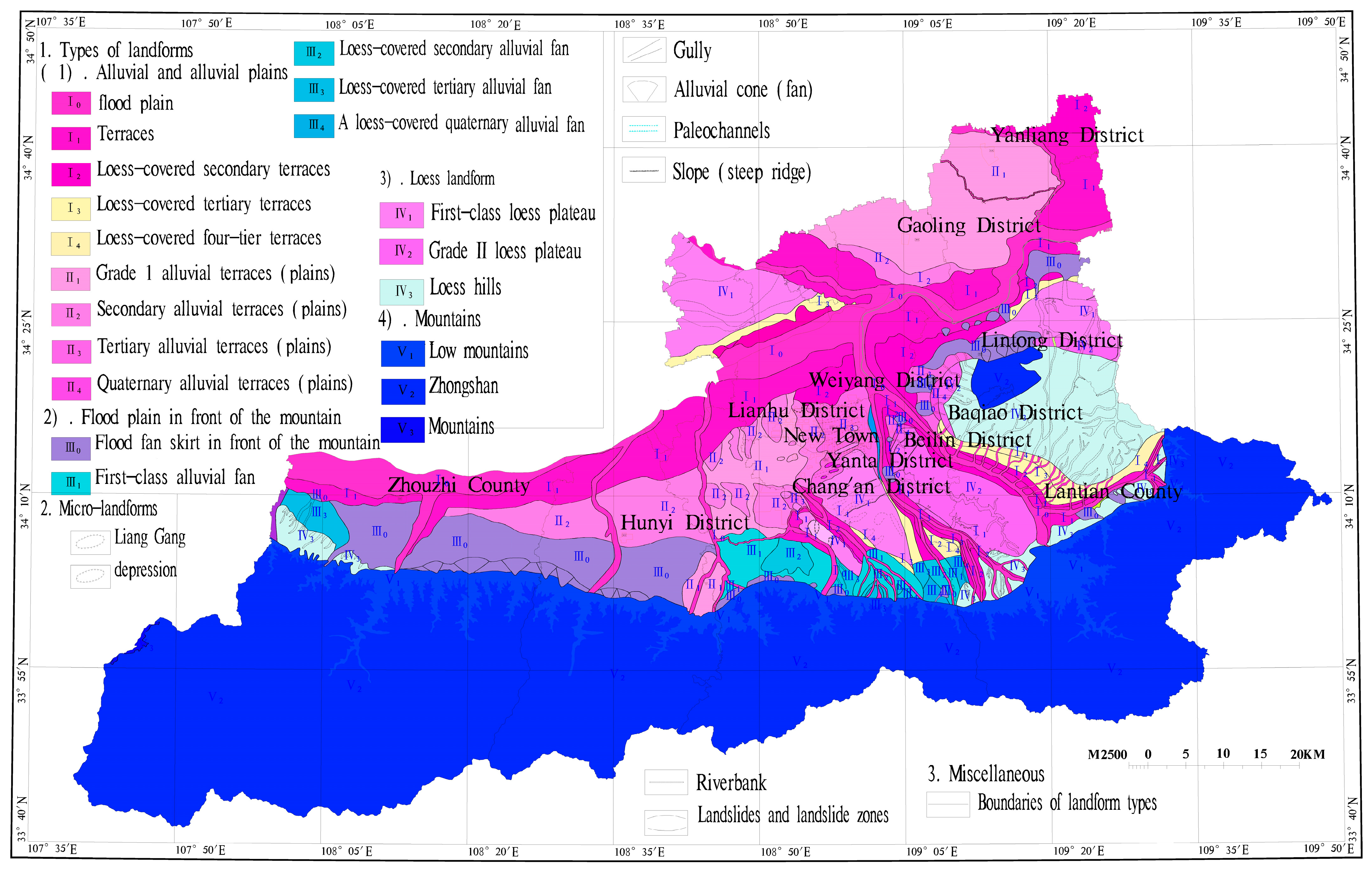
Geosciences 15 00290 g002
Figure 3. A topographic and geomorphological map of the study area.
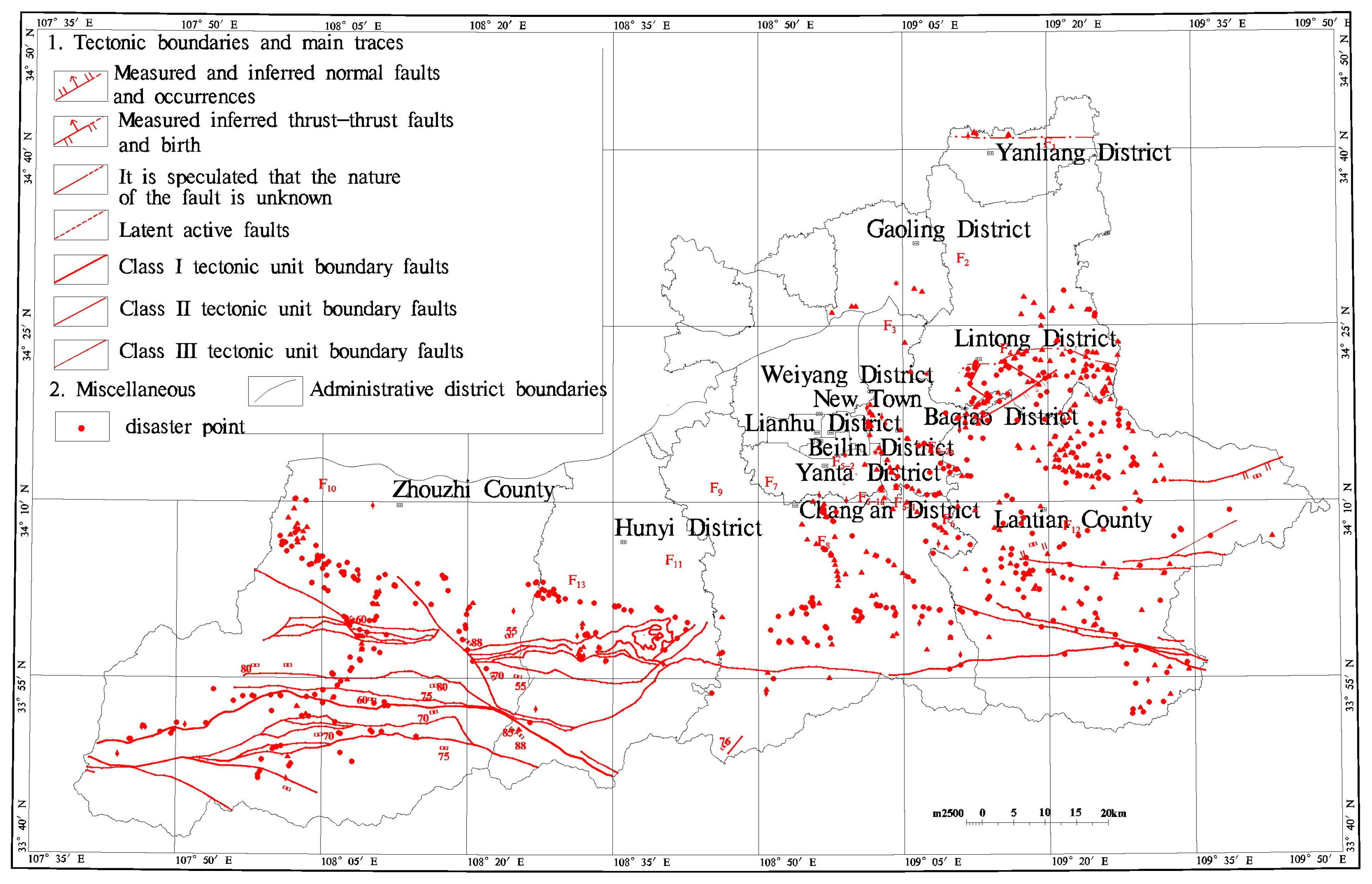
Geosciences 15 00290 g003
Figure 4. A geological structure map of the study area.
Geosciences 15 00290 g004
Figure 5. An engineering geological map of the study area.
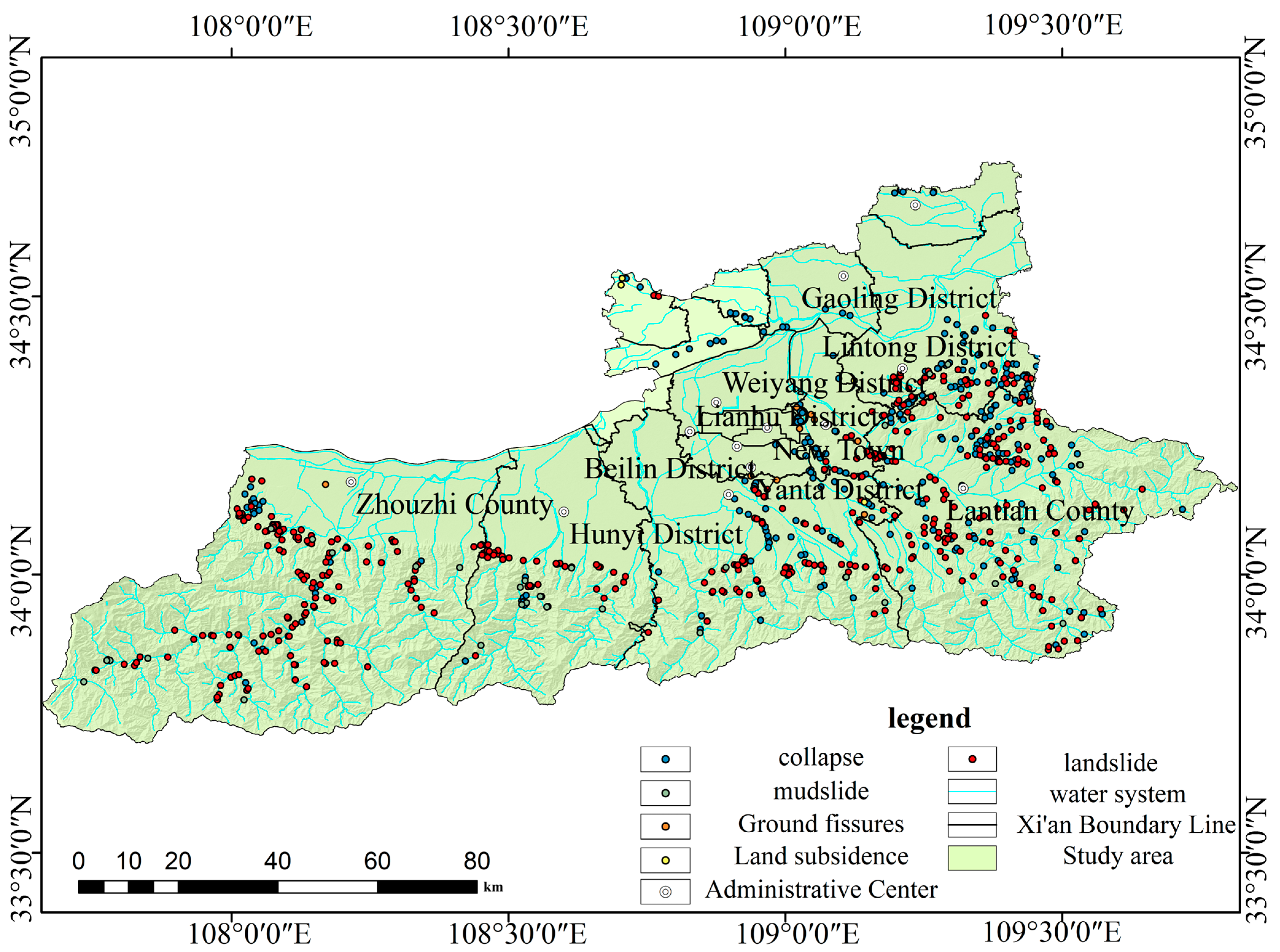
Geosciences 15 00290 g005
Figure 6. The distribution map of geological hazard hidden danger points in the study area.
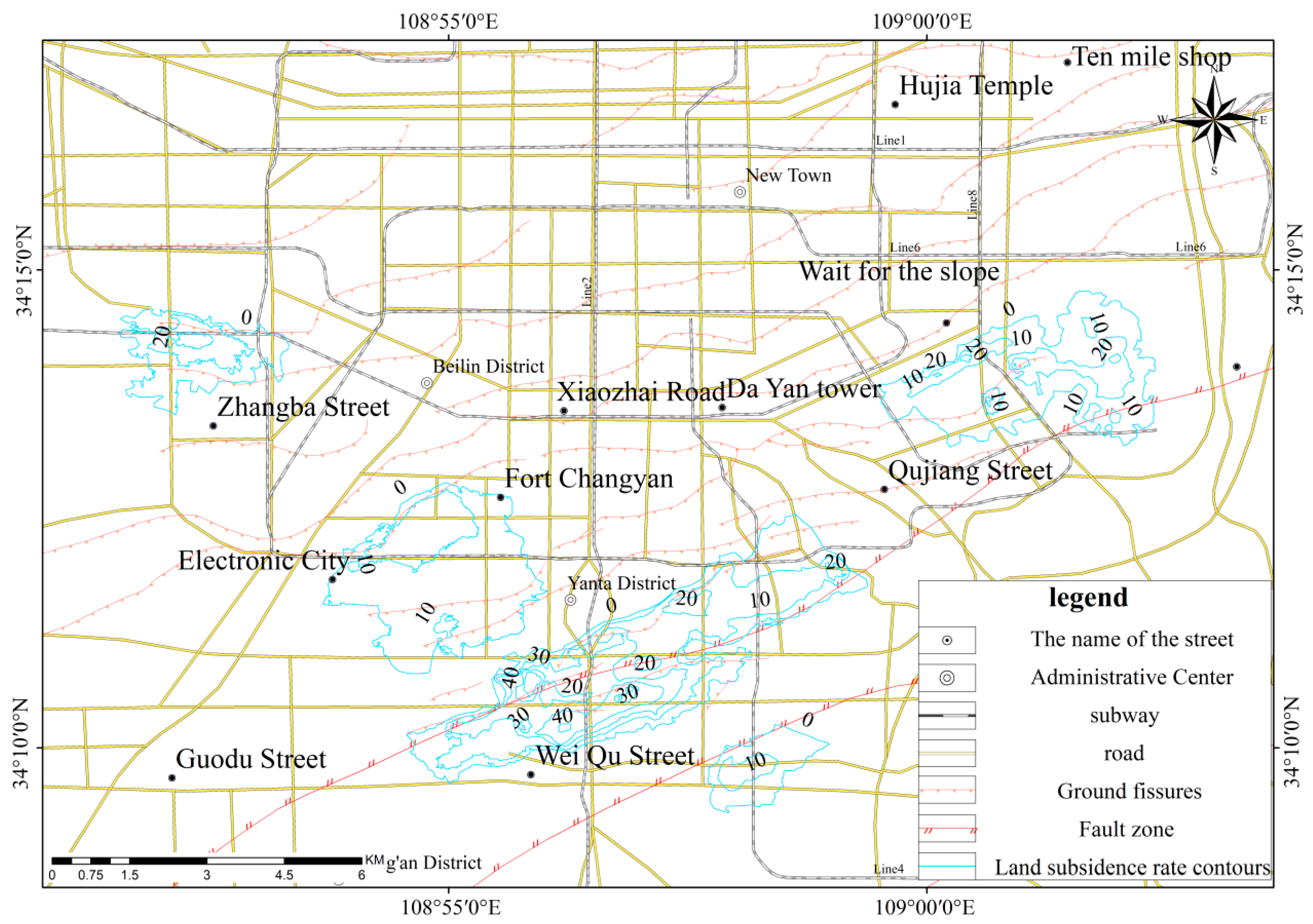
Geosciences 15 00290 g006
Figure 7. The ground subsidence rate contour map of the study area.
Geosciences 15 00290 g007
Figure 8. The cumulative ground subsidence contour map of the study area.
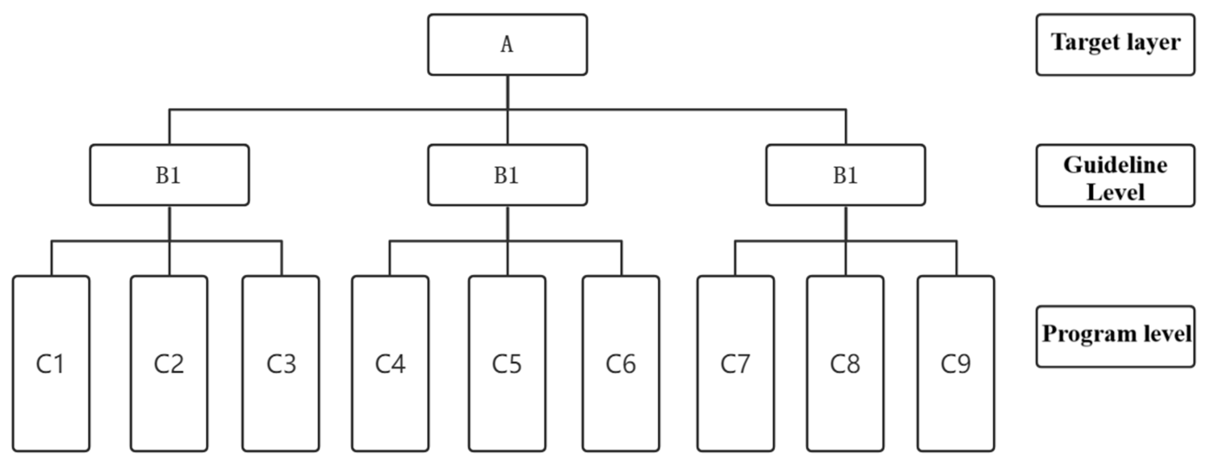
Geosciences 15 00290 g008
Figure 9. A schematic diagram of the analytic hierarchy process model.
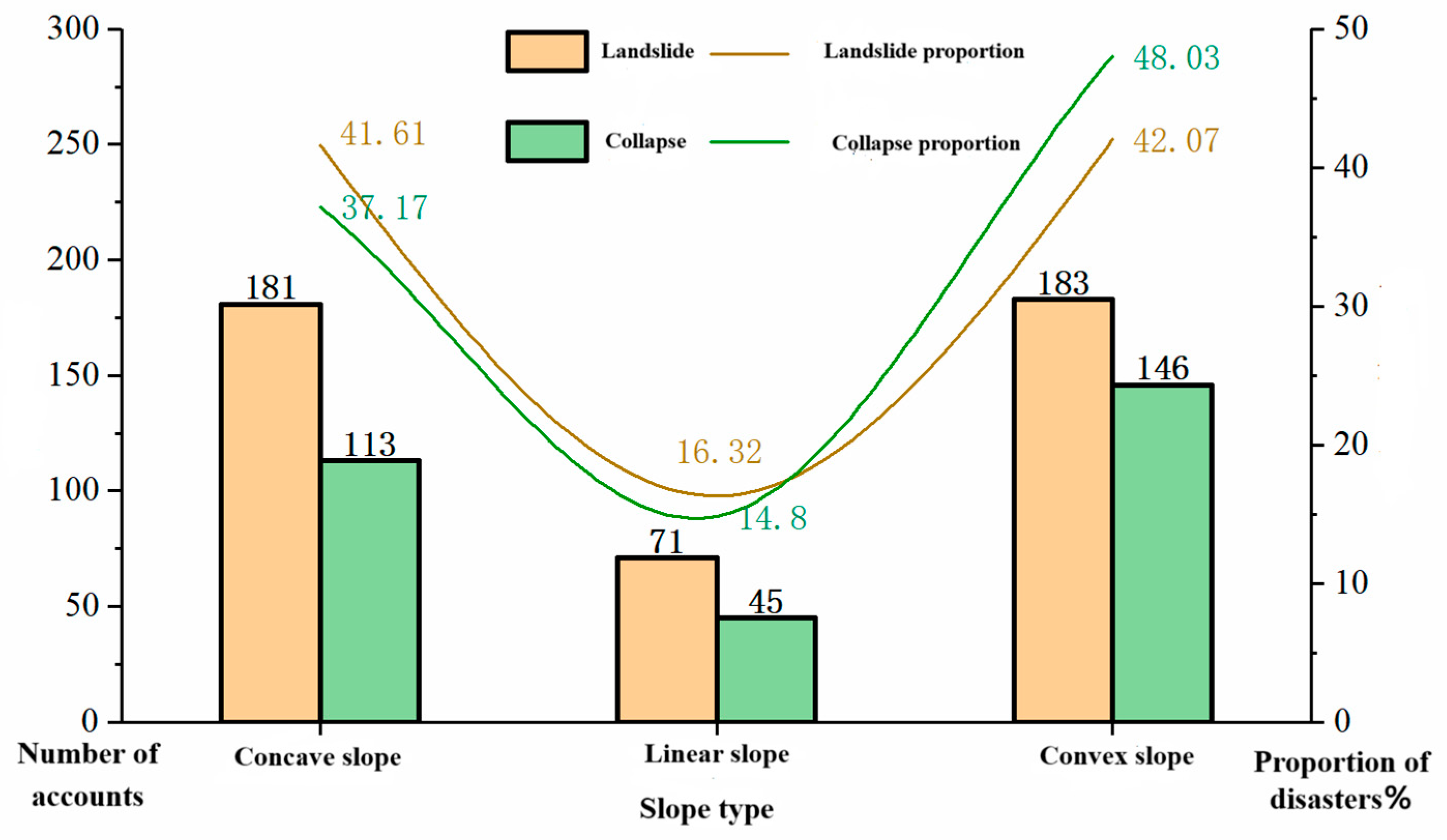
Geosciences 15 00290 g009
Figure 10. A diagram of the relationship between the number of landslides and collapse hazards and slope profile types.
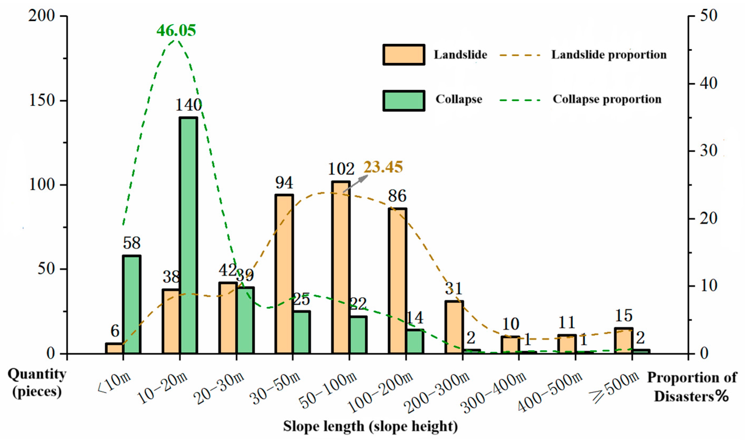
Geosciences 15 00290 g010
Figure 11. A diagram of the relationship between the number of landslides and collapse hazards and slope length.
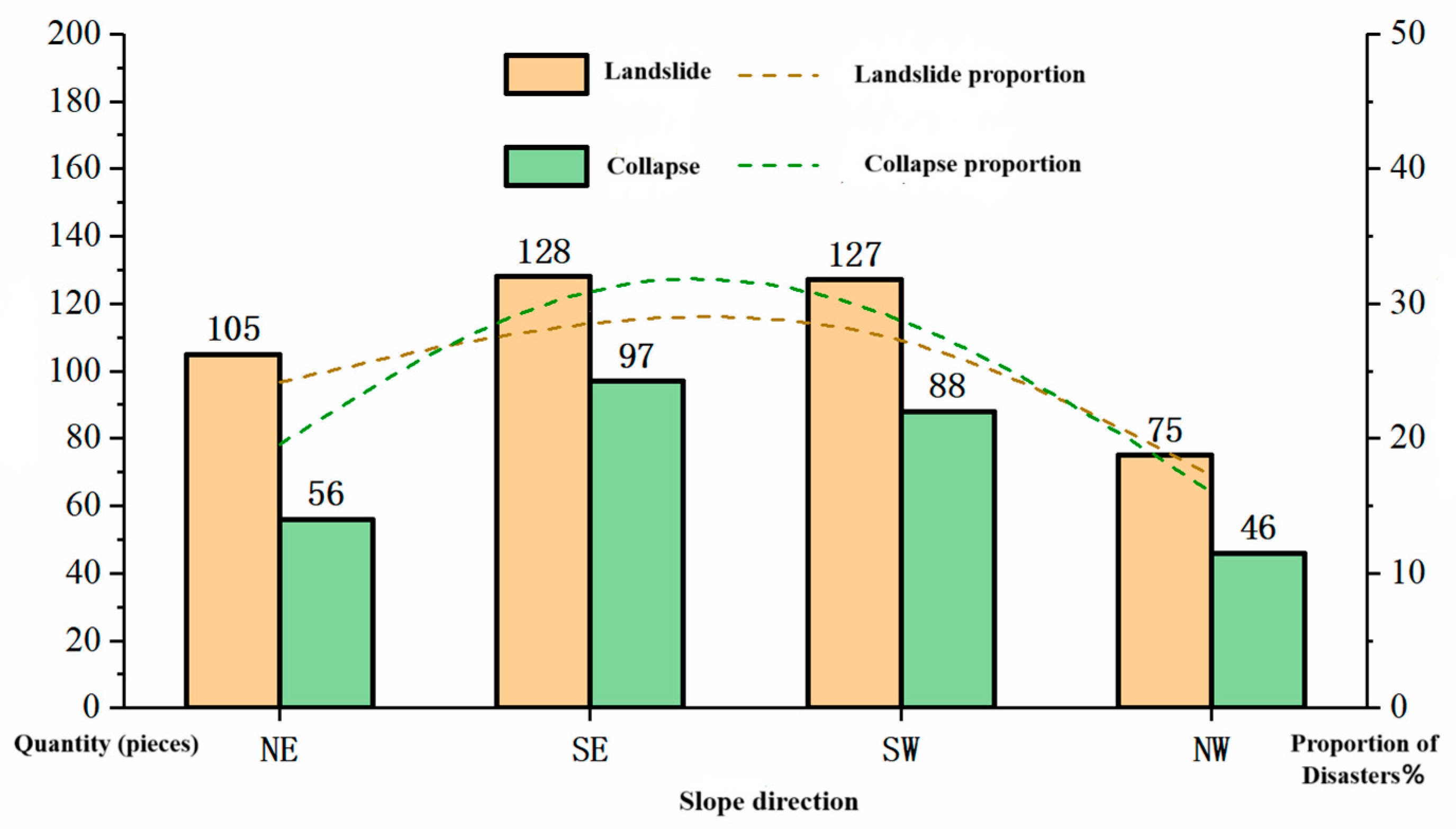
Geosciences 15 00290 g011
Figure 12. A diagram of the relationship between the number of landslides and collapse hazards and slope aspect.
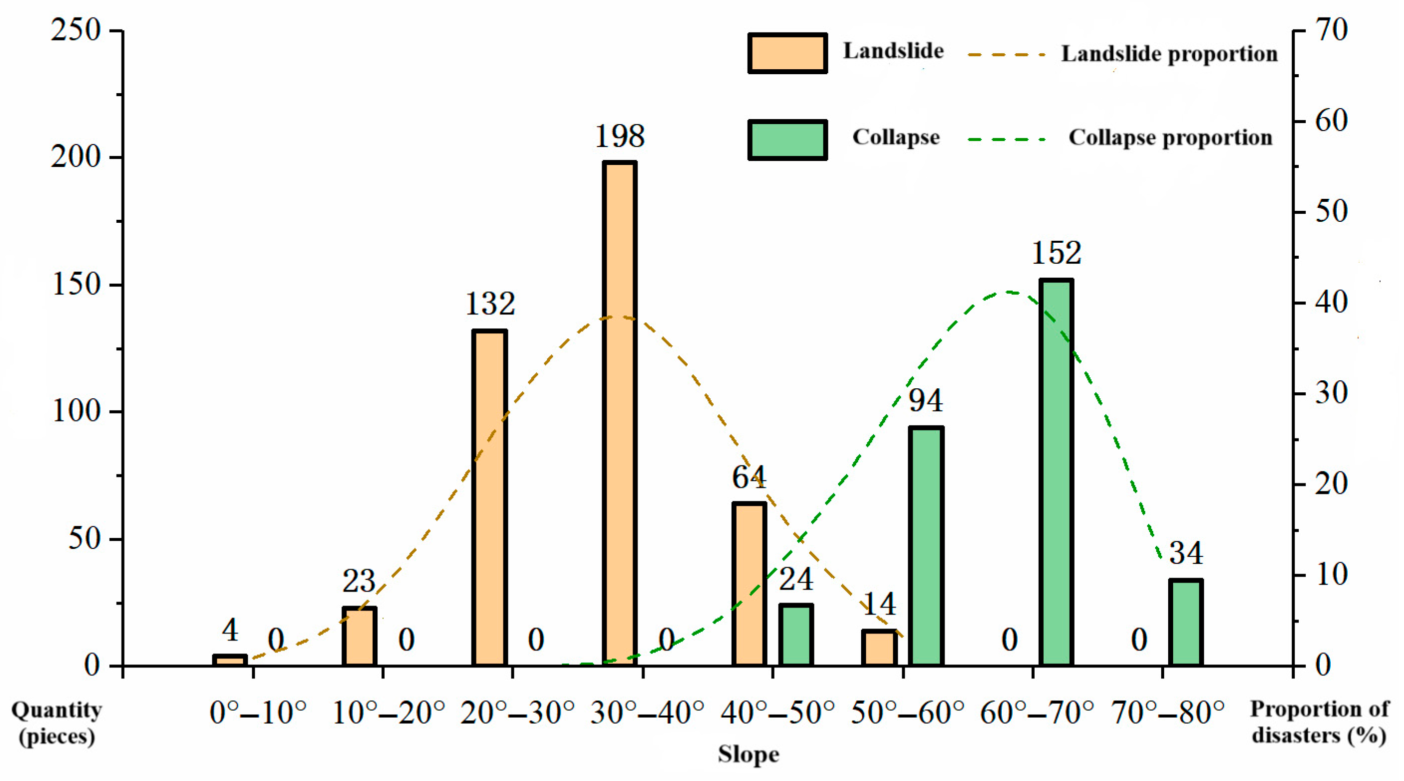
Geosciences 15 00290 g012
Figure 13. A diagram of the relationship between the number of landslides and collapse hazards and slope gradient.
Geosciences 15 00290 g013
Figure 14. A schematic diagram of the relationship between the geological structure and distribution of geological hazards.
Geosciences 15 00290 g014
Figure 15. Slope gradient classification map.
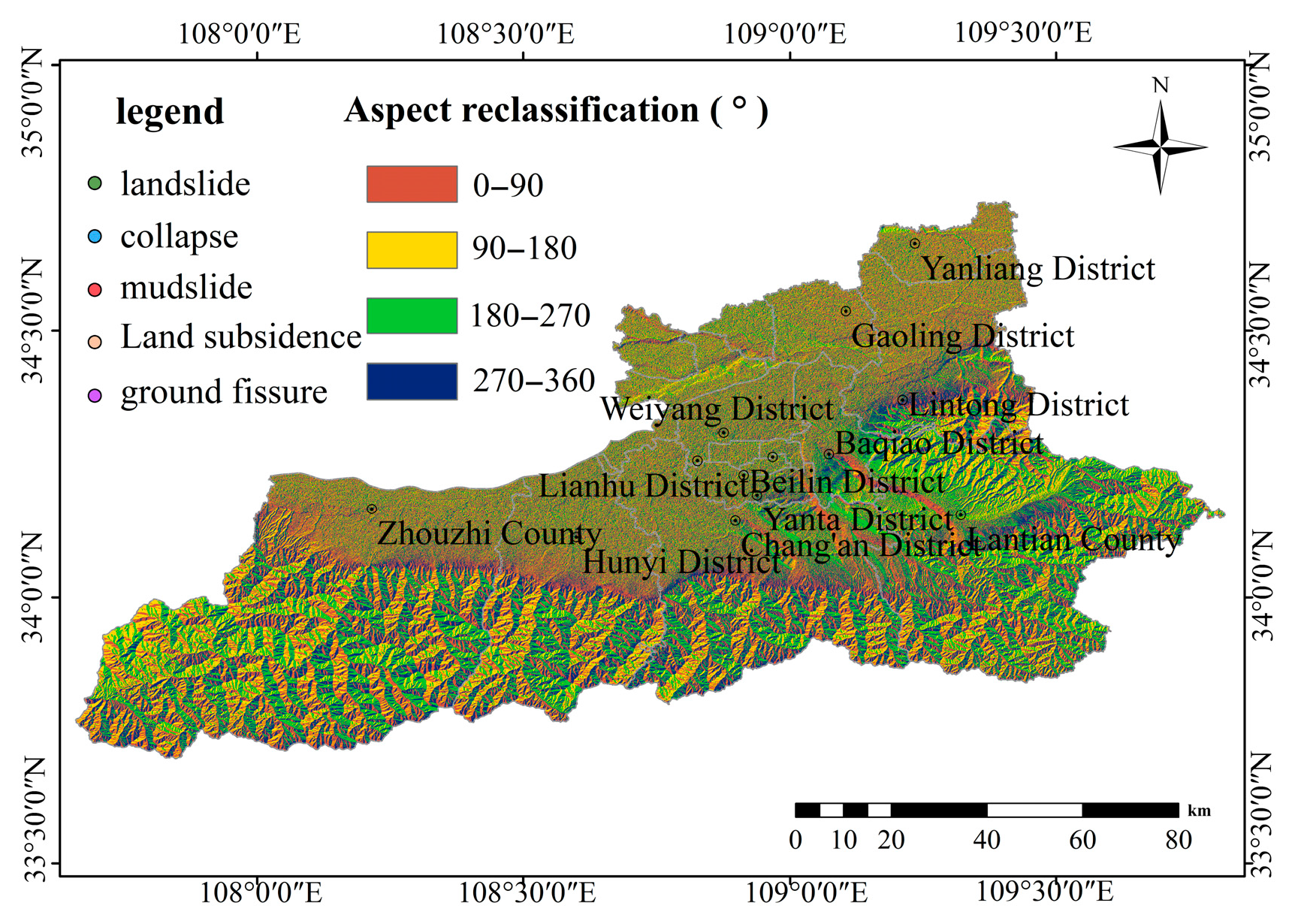
Geosciences 15 00290 g015
Figure 16. Slope aspect classification map.
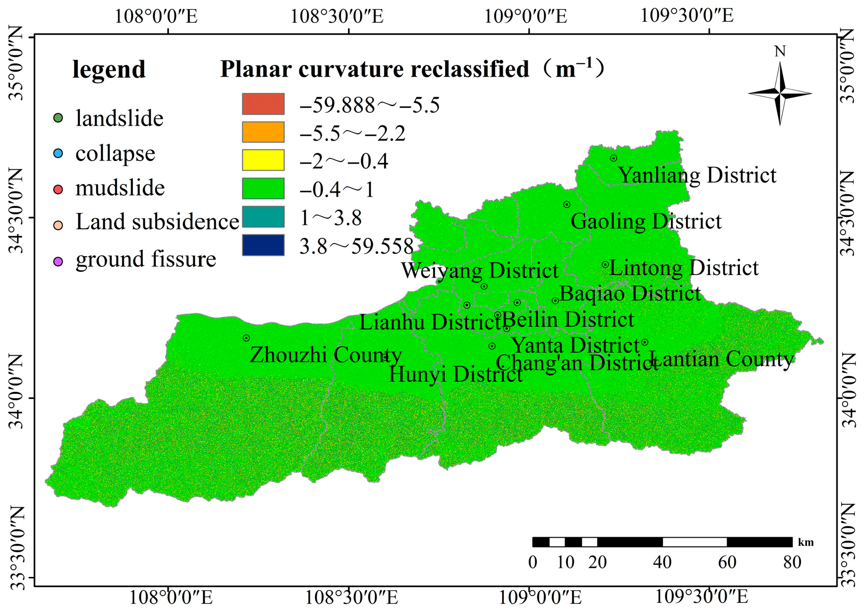
Geosciences 15 00290 g016
Figure 17. Plan curvature classification map.
Geosciences 15 00290 g017
Figure 18. Planar curvature classification map.
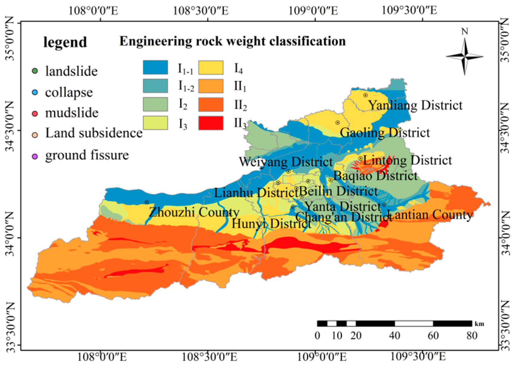
Geosciences 15 00290 g018
Figure 19. Rock and soil mass type classification map.
Geosciences 15 00290 g019
Figure 20. Profile curvature classification map.
Geosciences 15 00290 g020
Figure 21. Distance to fault classification map.
Geosciences 15 00290 g021
Figure 22. Distance to drainage system classification map.
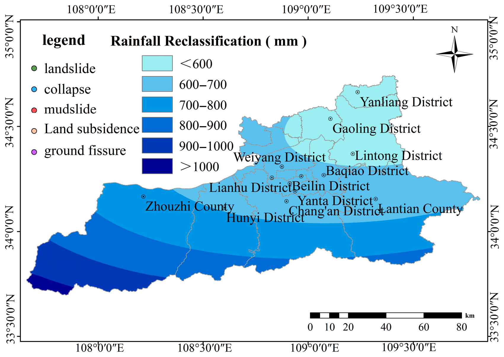
Geosciences 15 00290 g022
Figure 23. Rainfall classification map.
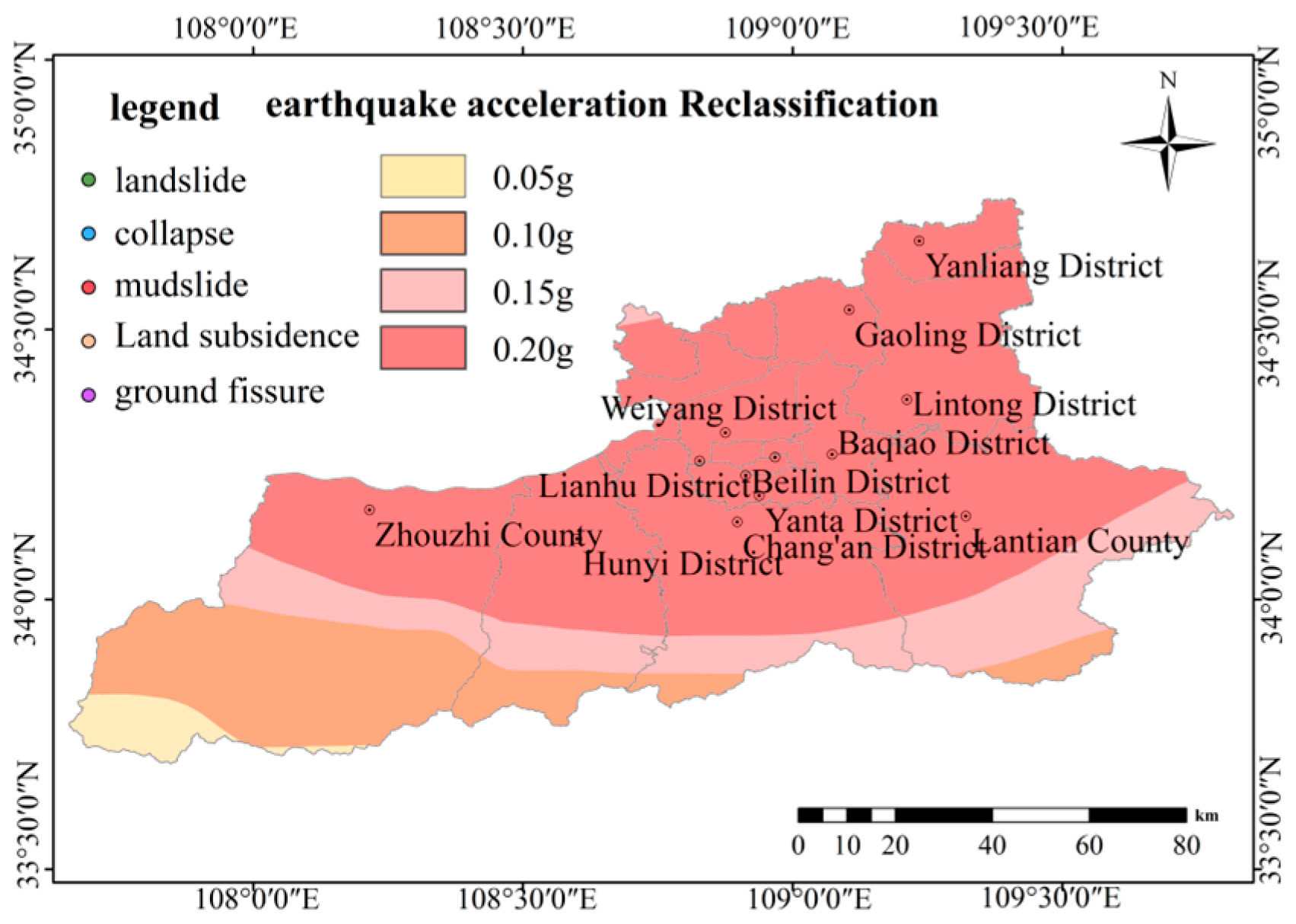
Geosciences 15 00290 g023
Figure 24. Seismic acceleration classification map.
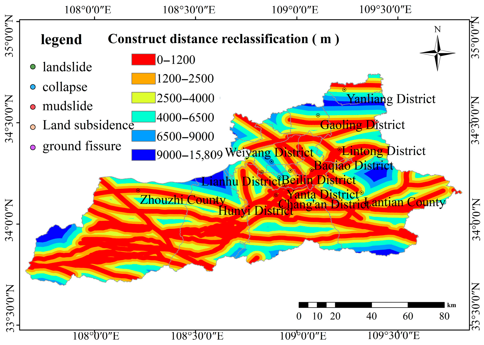
Geosciences 15 00290 g024
Figure 25. Distance to road classification map.
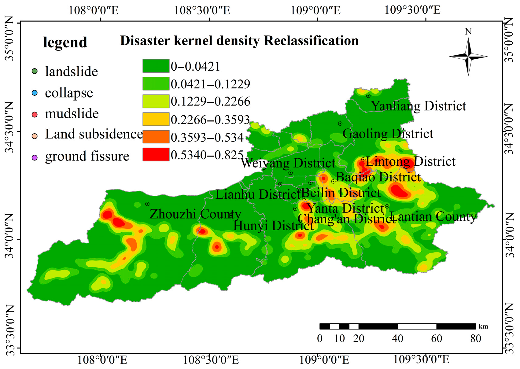
Geosciences 15 00290 g025
Figure 26. Hazard point kernel density classification map.
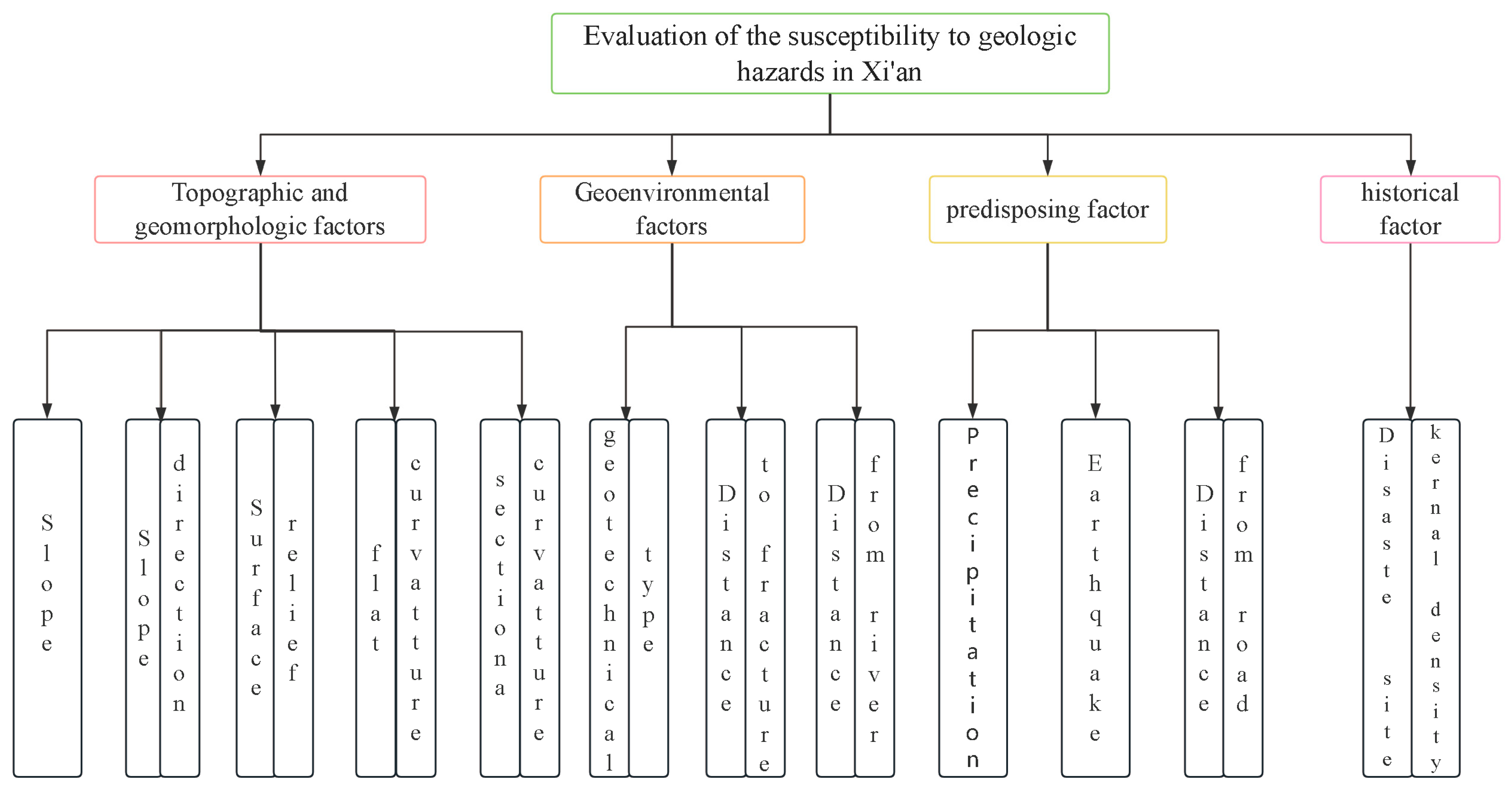
Geosciences 15 00290 g026
Figure 27. A diagram of the analytic hierarchy process system.
Geosciences 15 00290 g027
Figure 28. The evaluation results map generated using the unweighted information value method.
Geosciences 15 00290 g028
Figure 29. The evaluation results map generated using the subjective weighted information value method.
Geosciences 15 00290 g029
Figure 30. The evaluation results map generated using the objective weighted information value method.
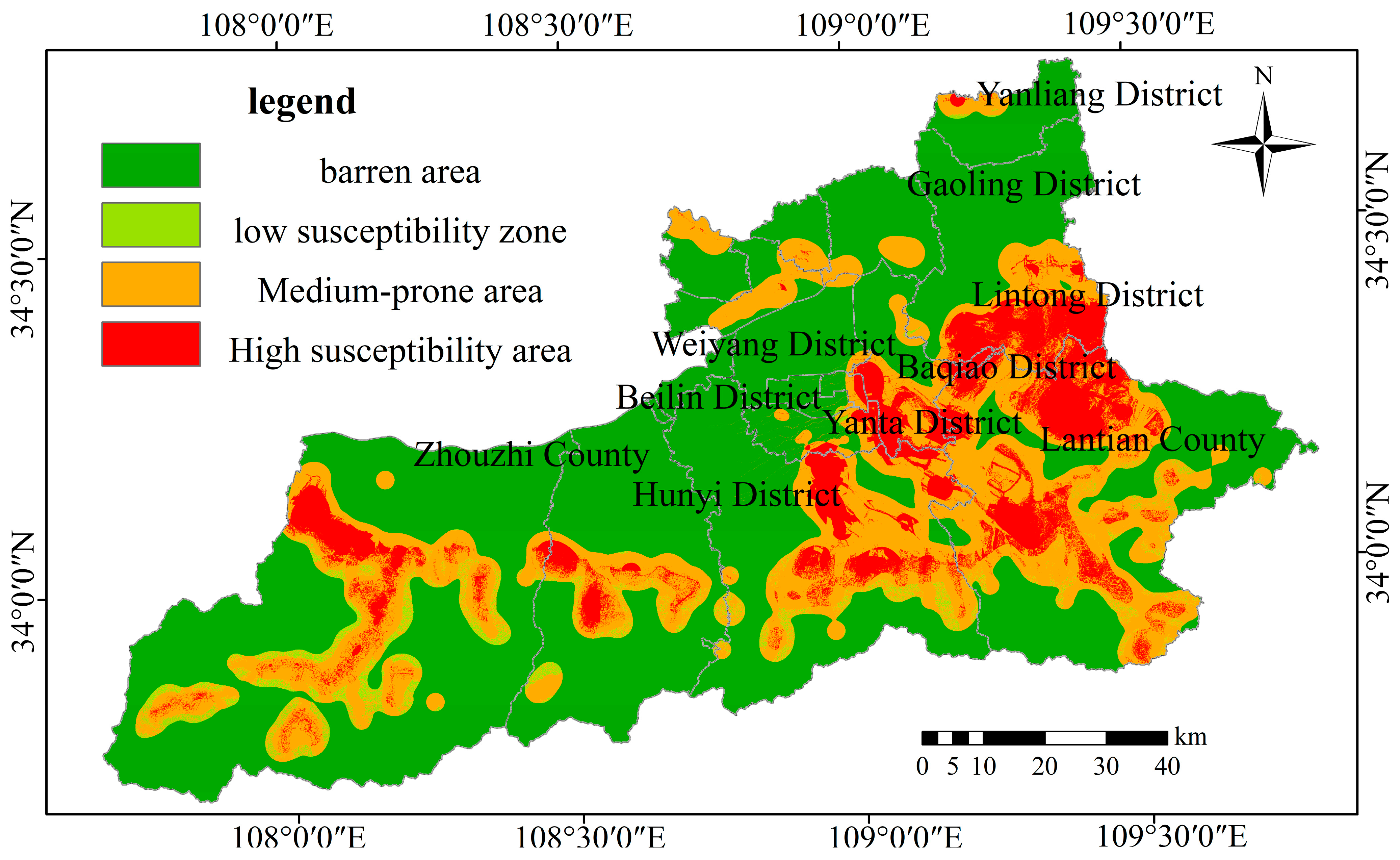
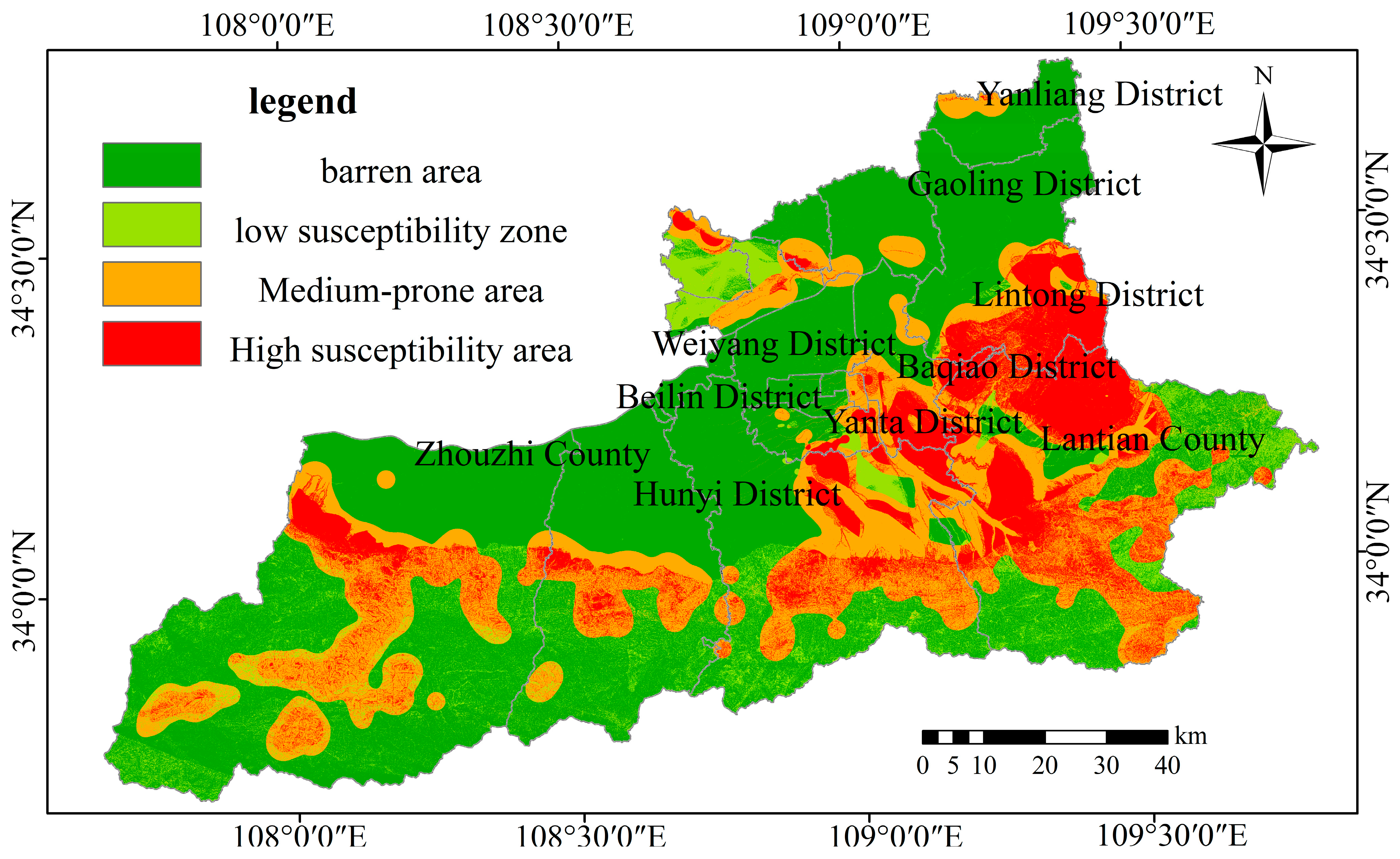
Geosciences 15 00290 g030
Figure 31. The evaluation results map generated using the comprehensive weighted information value method.
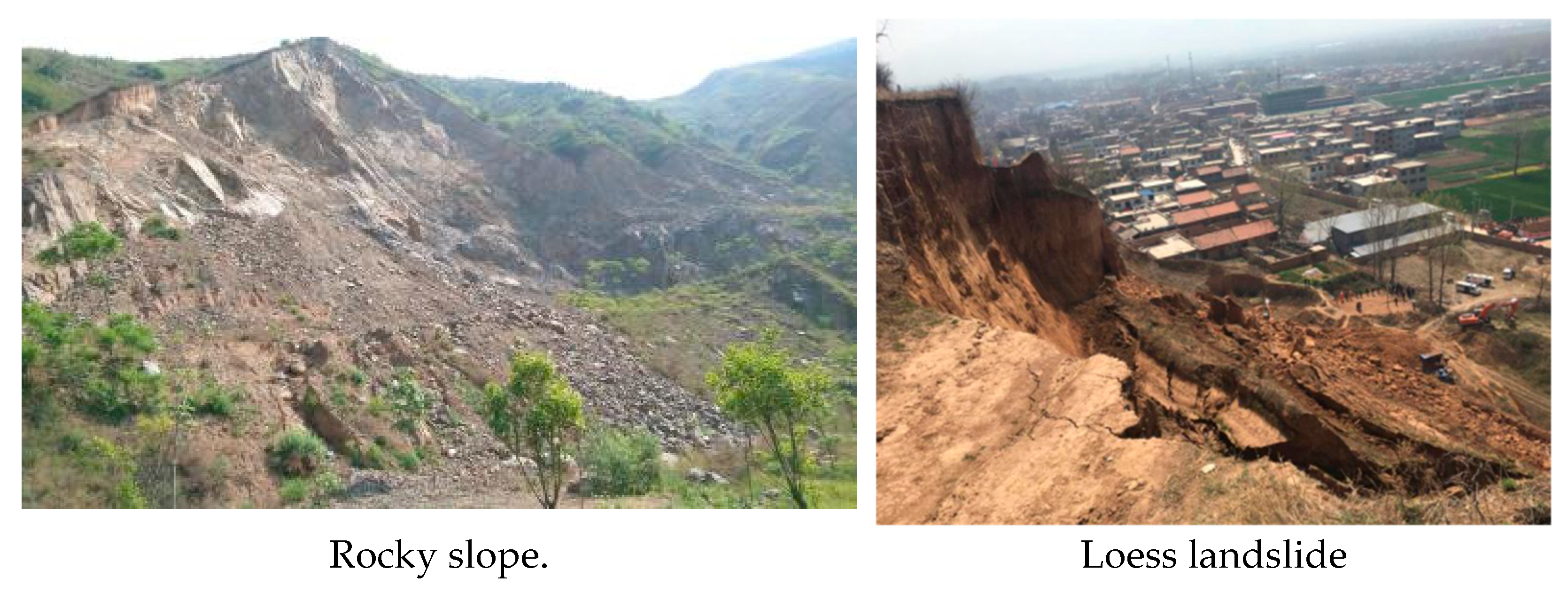
Geosciences 15 00290 g031
Figure 32. Photos of high-risk areas.
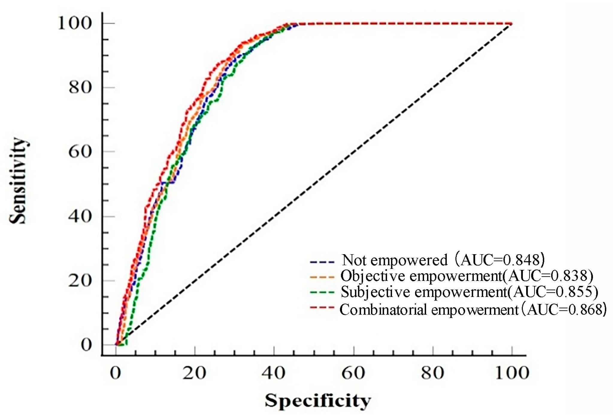
Geosciences 15 00290 g032
Figure 33. A comparison of ROC curves for different weighting models.
Geosciences 15 00290 g033
Table 1. The stratigraphic and lithological characteristics of the study area.
BoundarySystemFormation ComplexDescription
Neoarchean Taihua GroupExposed in Lishan of Lintong and west of Bayuan Town in Lantian County, uplifted to the surface by fault block action. The lithological structure is mainly composed of gneiss.
Paleoproterozoic Tietonggou FormationExposed in Bayuan Town and Lanqiao Town of Lantian County and Lishan area of Lintong District. The lithology is mainly metamorphic clastic rocks.
Guozhuang Rock FormationMainly distributed in the Qinling Mountains, with original rocks mainly composed of terrigenous clastic rocks.
Yanlinggou Rock FormationMainly distributed in Qinggangbian of Huyi District and west of Chenhe Town in Zhouzhi County, with lithology mainly composed of carbonate rocks.
Shangdianfang Rock FormationMainly distributed around Shangdianfang in Taibai County, sporadically distributed with small area, classified as metamorphism of greenschist and amphibolite facies.
Paleoproterozoic Dizhuanggou Rock FormationMainly distributed at the southwestern boundary of Houzhenzi Town in Zhouzhi County, appearing as elongated strips with small area.
Shaba and Heilongtan Formation
Group Combined Layer
Only exposed 9.0–13.9 km south of Houzhenzi Town in Zhouzhi County, comprising small area.
Neoproterozoic Xiong’er FormationDistributed in Bayuan Town of Lantian County, mainly volcanic rocks interbedded with terrigenous clastic rocks.
Guangdongping Rock FormationExposed between Mazhao Town and Chenhe Town in Zhouzhi County, distributed in east–west bands. The lithology is mainly metamorphic volcanic rocks.
Sichakou Rock FormationExposed in Pangguang Town of Huyi District, distributed in east–west bands, representing a suite of volcanic–sedimentary to terrigenous sedimentary clastic rocks.
Songshugou Rock FormationDistributed as remnant blocks south of Huangcaopo in Heihe, Zhouzhi, and north of Wangjihe Town. The rock characteristics are mainly metamorphic basic volcanic rocks interbedded with minor clastic rocks.
Lower Paleozoic Danfeng Rock FormationExtends from Houzhenzi Town to Wangjihe Town in Zhouzhi County in elongated strips, representing a tectonic mélange located in the main plate suture zone.
Luohansi Rock FormationExtends from Houzhenzi Town in Zhouzhi County to Huyi District, with main lithology including sandstone, carbonate rocks, and volcaniclastic rocks.
Erlangping Rock FormationDistributed in all four southern counties in elongated strips. The lithology is mainly volcanic rocks.
Taowan Rock FormationExposed near Lanqiao Town in elongated strips, with lithology mainly comprising metamorphic rocks, containing clastic rocks, clay rocks, and carbonate rocks.
Upper PaleozoicDevonianFenbiigou FormationMainly exposed in Shouyang Mountain of Zhouzhi County. The lithology is mainly metamorphic clastic rocks.
Chigou FormationExposed in Situn Town of Zhouzhi County, elongated strips trending NWW. The lithology is mainly sandstone with minor slate and phyllite.
Qingshiya FormationExposed in Situn Town and Wangjihe Town of Zhouzhi County. The lithology is mainly clay rocks interbedded with carbonate rocks and clastic rocks.
Tongyusi FormationExposed south of Situn Town in Zhouzhi County, with lithology mainly clastic rocks interbedded with clay rocks and minor carbonate rocks.
Dafenggou FormationDistributed around Situn Town in Zhouzhi County, with lithology mainly comprising sandstone in littoral facies.
Gudaoling FormationMainly distributed around Situn Town in Zhouzhi County, with lithology mainly comprising carbonate rocks interbedded with clay rocks and fine clastic rocks.
CarboniferousEryuhe FormationExposed around Xiaowangjian in Zhouzhi. The lithology is mainly carbonaceous slate interbedded with gravel-bearing quartz sandstone and siltstone.
PermianShihezi FormationDistributed in Chenhe Town of Zhouzhi County, extending in east–west bands. The lower lithology is mainly mudstone and sandstone; the upper part consists of fine sandstone and sandy and argillaceous mudstone.
MesozoicTriassicWulichuan FormationDistributed near Liuyehe in Zhouzhi and Pengjiawan in Lantian County. The lower lithology is mainly quartz conglomerate; the upper part consists of sandy slate and quartz sandstone.
CretaceousDonghe FormationDistributed around Situn Town in Zhouzhi County. The lithology is mainly clastic rocks.
CenozoicPaleogeneHonghe FormationExposed in the middle and upper reaches of various gullies in Lishan, with lithology mainly comprising mudstone interbedded with sandstone and siltstone.
Bailuyuan FormationExposed near Bailuyuan, with lithology mainly comprising sandstone interbedded with mudstone and sandstone.
CenozoicPaleogeneGanhe FormationMainly sandstone and sandy conglomerate, interbedded with argillaceous rocks.
NeogeneLengshuigou FormationDistributed around Lantian. The lithology is mainly sandy mudstone interbedded with sandstone, with conglomerate at the bottom.
Koujiagcun FormationMainly exposed in Maodong Village, Baqiao District, Xi’an. The lithology is mainly mudstone and sandy mudstone.
Bahe FormationMainly distributed in Lantian County and Lintong District. The lithology is mainly mudstone and sandy mudstone.
Lantian FormationMainly distributed around Lantian. The lithology is mainly clay rocks and sandy clay rocks.
QuaternaryGlaciofluvial DepositsMainly distributed near Gongwangling in Lantian County and valley exits at the front of the Qinling Mountains. The lithology is mainly sandy gravel.
Eolian DepositsMainly distributed in Bailuyuan, with lithology of loess containing calcareous nodules and multiple paleosol layers.
Eolian DepositsMainly distributed in the northern loess hilly area and tableland area of Lantian County. The lithology is mainly sandy gravel layers and paleosols, containing calcareous nodules and interbedded with multiple paleosol layers.
Proluvial DepositsOnly exposed at the proluvial fan south of Yangzhuang Subdistrict in Chang’an District, with small distribution area. Mainly sandy gravel, boulders, and silty clay layers.
Eolian DepositsLarge distribution area, commonly called “Malan Loess”.
MoraineLocated around Taibai Mountain, formed by accumulation of materials transported in different ways after glacier melting. Composed of clastic materials with extremely poor sorting, poor roundness, and no directional arrangement.
Landslide Gravity DepositsDistributed in Dizhai Subdistrict of Baqiao District, with material composition mainly comprising loess and paleosols containing calcareous nodules.
Alluvial–Proluvial DepositsMainly distributed in Yanliang District and Gaoling District. The material composition is mainly fine- to medium-coarse sand and silty clay layers.
Proluvial DepositsMainly distributed at the front of Qinling Mountains and Lishan, with material composition mainly comprising sandy gravel, boulders, and silty clay layers.
Alluvial DepositsWidely distributed, located at the same position as the first geomorphological terrace, with material composition mainly comprising sand, sandy gravel, and silty clay layers.
Proluvial DepositsMainly distributed at the front of Qinling Mountains and Lishan, with material composition mainly comprising sandy gravel, boulders, and silty clay layers.
Alluvial DepositsWidely distributed, located at the same position as geomorphological floodplains, with material composition mainly comprising sand, sandy gravel, and silty clay layers.
Table 2. A statistical table of sudden-onset geological hazard types.
No.Sudden-Onset Geological HazardsClassification CriteriaQuantity (Locations)Percentage
1LandslidesMaterial CompositionLoess landslides20647.36%
Accumulation layer landslides21048.28%
Rock landslides194.36%
ScaleSmall33476.78%
Medium6314.48%
Large317.13%
Extra-large61.38%
Giant10.23%
Profile MorphologyConvex18141.61%
Concave18342.07%
Linear7116.32%
2CollapsesMaterial CompositionLoess collapses24279.61%
Accumulation layer collapses144.60%
Rock collapses4815.79%
ScaleSmall22875.00%
Medium6421.05%
Large103.29%
Extra-large10.66%
3Ground CollapseScale TypeSmall787.50%
Medium00.00%
Large112.50%
4MudslideBasin MorphologyHillslope-type debris flows1136.67%
Valley-type debris flows1963.33%
Deposit VolumeSmall2170.00%
Medium826.67%
Large00.00%
Extra-large13.33%
Notes: Small landslide: Landslide volume is less than 10 × 104 cubic meters. Medium-sized landslide: Landslide volume is 10 × 104~100 × 104 cubic meters. Large landslide: Landslide volume is 100 × 104~1000 × 104 cubic meters.
Table 3. Scale values and their meanings.
Scale (Cij)Meaning
1Factors i and j are equally important
3Factor i is slightly more important than factor j
5Factor i is obviously more important than factor j
7Factor i is significantly more important than factor j
9Factor i is extremely more important than factor j
2, 4, 6, 8Importance levels are in intermediate states
Reciprocals of the above scale valuesRepresent the degree of importance of factor j compared to factor i
Table 4. Judgment Matrix C.
CC1C2C3……Cn
C1c11c12c13……c1n
C2c21c22c23……c2n
C3c31c32c33……c3n
………………………………
Cncn1cn2cn3……cnn
Table 5. The average randomized consistency indicator RI value.
n123456789101112131415
RI000.520.891.121.261.361.411.461.491.521.541.561.581.59
Table 6. The regional distribution of geological hazard hidden danger points.
RegionNumber of Geological Hazard Hidden Danger PointsPercentage of Total Disaster PointsDisaster Point Quantity Ranking
LandslidesCollapsesMudslideGround CollapseGround FissuresTotal
Lantian County1228630021126.81%1
Zhouzhi County14422100117722.49%2
Chang’an District675861313517.15%3
Lintong District455821010613.47%4
Baqiao District1640014617.75%5
Huyi County378900546.86%6
Xixian New Area413020192.41%7
Yanliang District0600281.02%8
Gaoling District0501060.76%9
Chanba Ecological District0401050.64%10
Yanta District0301040.51%11
International Port District0100010.13%12
Total43530430810787
Table 7. A table of the relationship between geological hazard quantities and geomorphological types.
Hazard TypeNumber of Hazard PointsTotal
Alluvial and Alluvial–Pluvial PlainsPiedmont Pluvial Plain AreasLoess Landform AreasMountainous Regions
Landslides315136263435
Collapses611715076304
Debris Flows-122730
Ground Collapse6-2-8
Ground Fissures8-2-10
Total10623292366787
Table 8. A statistical table of the relationships between geomorphological types and geological hazards.
Geomorphological TypeArea (km2)Geological Hazard Points
NumberPercentage
Alluvial and Alluvial–Pluvial Plain Areas3188.0810613.47%
Piedmont Pluvial Plain Areas873.96232.92%
Loess Landform Areas1279.1029237.10%
Mountainous Regions5248.2036646.51%
Table 9. A statistical table of distribution quantities of geological hazard hidden danger points in different stratigraphic ages.
Stratigraphic AgeLandslidesCollapsesMudslidesGround CollapseGround FissuresTotalPercentage
Quaternary156173581035244.73%
Neogene3223000556.99%
Paleogene32461007910.04%
Upper Paleozoic4114400597.50%
Middle Paleozoic181100202.54%
Lower Paleozoic68199009612.19%
Proterozoic731410009712.33%
Neoarchean1514000293.68%
Total43530430810787
Table 10. A statistical table of geological hazard quantities in different rock and soil mass zones.
Rock and Soil Mass Zone CodeArea (km2)Geological Hazard Types
CollapsesLandslidesDebris FlowsGround CollapseGround Fissures
Silty clay + sandy gravel dual-layer structure zone (I1-1)1721.614012-12
Loess (interbedded with paleosol) + sand, sandy gravel dual-layer structure zone (I1-2)410.782519-12
Loess (interbedded with paleosol) single-layer structure zone (I2)1291.64148139332
Loess, loess-like soil, and sandy gravel multi-layer structure zone (I3)717.93115-32
Sandy gravel, sandy clay multi-layer structure zone (I4)1416.82792-2
Massive hard intrusive rock engineering geological zone (II1)2236.6730808--
Massive hard to moderately hard intermediate to high-grade metamorphic rock engineering geological zone (II2)2451.273514316--
Layered moderately hard to weak sedimentary rock engineering geological zone (II3)342.178281--
Total10,588.930443530108
Table 11. A classification and statistical table of factors influencing geological hazards.
Influencing FactorClassificationArea (km2)Hazard PointsInfluencing FactorClassificationArea (km2)Hazard Points
Slope Gradient (°)0~105231.64Rock and Soil Mass TypesI1-11721.5955
10~201157.6223I1-2410.7847
20~301610.37132I21291.66295
30~401616.81198I3717.9421
40~50794.21588I41416.8320
50~60171.923108II12236.68118
60~7023.43152II22469.88194
70~801.55834II3342.1737
80~900.0060Distance to Faults (m)0~12003638.99388
Slope Aspect (°)0~903390.91771200~25002533.83170
90~1802322.282382500~40001913.1487
180~2702399.082374000~65001586.7277
270~3602495.271356500~9000616.7641
Surface Relief0~75484.4413329000~15,809.26318.0824
7~161916.21324Hazard Point Kernel Density (points/km2)0~0.0426501.61
16~241744.91920.042~0.1231823.7290
24~341079.1270.123~0.2271237.4196
34~50335.071100.227~0.359602.78189
50~24547.79820.359~0.534312.78179
Rainfall (mm)<6003638.991300.534~0.825129.25132
600~7002533.83302Plan Curvature−59.888~−5.571.36022
700~8001913.14260−5.5~−2.2430.26531
800~9001586.7270−2.2~−0.42513.08221
900~1000616.7625−0.4~16170.73426
>1000318.0801~3.81232.895
3.5~59.558189.29612
Distance to Drainage Systems0~3002261.27240Profile Curvature−80.939~−5.3145.6996
300~5001355.63110−5.3~−1.9576.34849
500~10002853.92201−1.9~−0.13547.06235
1000~30003662.43220−0.1~1.55379.03398
3000~5000416.032151.5~5.0791.5991
5000~7574.2158.236615.0~65.145167.8048
Earthquake<0.05264.7961Distance to Roads0~50304.46256
0.05~0.101826.718750~150581.768104
0.10~0.201637.6480150~250511.70483
>0.206878.37619250~5001101156
500~10001641.95169
>10006466.64219
Table 12. Weight coefficient values obtained using the analytic hierarchy process.
IndicatorABCDEFGHIJKL
Weight0.1020.0180.1020.0180.0180.0400.0700.0290.1310.0550.1700.247
Note: A represents slope gradient, B represents slope aspect, C represents surface relief, D represents plan curvature, E represents profile curvature, F represents rock and soil mass types, G represents the distance to faults, H represents the distance to drainage systems, I represents rainfall, J represents earthquake intensity, K represents the distance to roads, and L represents the hazard point kernel density.
Table 13. Weight coefficient values obtained using the entropy weight method.
IndicatorABCDEFGHIJKL
Weight0.1370.1240.1630.0170.0180.1450.0260.0090.1930.0270.0060.135
Note: A represents slope gradient, B represents slope aspect, C represents surface relief, D represents plan curvature, E represents profile curvature, F represents rock and soil mass types, G represents the distance to faults, H represents the distance to drainage systems, I represents rainfall, J represents earthquake intensity, K represents the distance to roads, and L represents the hazard point kernel density.
Table 14. Combined weighting weight coefficient values.
IndicatorABCDEFGHIJKL
Weight0.1160.0610.1270.0180.0180.0820.0520.0210.1560.0440.1040.201
Note: A represents slope gradient, B represents slope aspect, C represents surface relief, D represents plan curvature, E represents profile curvature, F represents rock and soil mass types, G represents the distance to faults, H represents the distance to drainage systems, I represents rainfall, J represents earthquake intensity, K represents the distance to roads, and L represents the hazard point kernel density.
Table 15. The information values of selected assessment indicators.
Factor TypeAssessment FactorValue RangeHazard Point ProportionArea ProportionHazard Point Density RatioInformation Value I
Topography and GeomorphologySlope Gradient (°)0~100.54%49.32%0.64−4.51
10~203.11%10.91%3.35−1.25
20~3017.86%15.18%1.330.16
Slope Aspect (°)0~9022.49%31.97%0.70−0.35
90~18030.24%21.89%1.380.32
Geological EnvironmentRock and Soil Mass TypesI1-16.99%16.23%0.43−0.84
I237.48%12.18%3.081.12
Triggering FactorsRainfall (mm)<60016.52%16.00%1.030.03
600~70038.37%32.77%1.170.16
Table 16. Total variance explained.
ComponentInitial EigenvaluesRotation Sums of Squared Loadings
TotalVarianceCumulativeTotalVarianceCumulative
13.23326.93826.9382.30819.23419.234
21.52312.69339.6312.25218.76938.003
31.35411.28550.9161.49212.43250.435
41.06910.90861.8241.0949.11759.551
51.0468.71670.5401.0798.98868.540
60.9497.91176.450
70.7916.59583.046
80.6905.75488.800
90.5114.26293.062
100.4633.85796.919
110.2642.20499.123
120.1050.877100.000
Table 17. Component matrix.
Component
12345
Slope0.310.71−0.340.13−0.57
Aspect−0.08−0.82−0.110.03−0.16
Relief amplitude0.560.77−0.050.14−0.057
Plan curvature−0.400.43−0.8570.01−0.051
Profile curvature−0.330.23−0.859−0.41−0.080
Engineering geological rock and soil type−0.480.130.610.580.04
Distance to fault structures0.240.190.30−0.890.27
Distance to river systems−0.0116−0.2030.430.130.20
Precipitation0.03980.2980.7980.300.91
Peak ground acceleration−0.36−0.1930.610.0800.34
Distance to roads0.470.06−0.430.760.27
Disaster point kernel density0.930.470.620.300.46
Table 18. Statistical table of hazard point density in different zones of various models.
Susceptibility ZoneUnweighted Information Value Subjective Weighted Information Value Objective Weighted Information Value Comprehensive Weighted Information Value
Number of Hazard PointsProportion (%)Number of Hazard PointsProportion (%)Number of Hazard PointsProportion (%)Number of Hazard PointsProportion (%)
Non-susceptible Area0010.120010.13
Low-Susceptibility Area20.2540.51182.2940.51
Moderate-Susceptibility Area25632.5323229.4826733.9220325.79
High-Susceptibility Area52967.2255069.8950263.7957973.57
Total787100787100787100787100
Disclaimer/Publisher’s Note: The statements, opinions and data contained in all publications are solely those of the individual author(s) and contributor(s) and not of MDPI and/or the editor(s). MDPI and/or the editor(s) disclaim responsibility for any injury to people or property resulting from any ideas, methods, instructions or products referred to in the content.

