Abstract
This study focuses on developing a climate-flood model to investigate and interpret the relationship and impact of climate on runoff/flooding at a sub-regional scale using multiple linear regression (MLR) with 30 years of hydro-climatic data for the Cross River Basin, Nigeria. Data were obtained from Nigerian Meteorological Agency (NIMET) for the following climatic parameters: annual average rainfall, maximum and minimum temperatures, humidity, duration of sunlight (sunshine hours), evaporation, wind speed, soil temperature, cloud cover, solar radiation, and atmospheric pressure. These hydro-meteorological data were analysed and used as parameters input to the climate-flood model. Results from multiple regression analyses were used to develop climate-flood models for all the gauge stations in the basin. The findings suggest that at 95% confidence, the climate-flood model was effective in forecasting the annual runoff at all the stations. The findings also identified the climatic parameters that were responsible for 100% of the runoff variability in Calabar (R2 = 1.000), 100% the runoff in Uyo (R2 = 1.000), 98.8% of the runoff in Ogoja (R2 = 0.988), and 99.9% of the runoff in Eket (R2 = 0.999). Based on the model, rainfall depth is the only climate parameter that significantly predicts runoff at 95% confidence intervals in Calabar, while in Ogoja, rainfall depth, temperature, and evaporation significantly predict runoff. In Eket, rainfall depth, relative humidity, solar radiation, and soil temperatures are significant predictors of runoff. The model also reveals that rainfall depth and evaporation are significant predictors of runoff in Uyo. The outcome of the study suggests that climate change has impacted runoff and flooding within the Cross River Basin.
1. Introduction
There are growing concerns about the impacts of climate change on flooding. The recent 2022 Nigerian floods, which impacted several regions of the country, were attributed to climate change. In response, the Federal Government of Nigeria established a Presidential Committee on Flooding with a task to develop a comprehensive flood management plan for Nigeria within 90 days. Variations in climatic conditions result in significant fluctuations in runoff [1] Although Nigeria is accustomed to seasonal flooding, the 2022 floods were the most severe in the country since the 2012 flood [2]. Incidences of flood disasters are increasing globally, with both regional and sub-regional flood intensities also on the rise. In 2022, persistent flood events reached a peak in Nigeria, affecting 19 states [2].
Flooding is caused by several factors, particularly runoff. Runoff refers to the flow of rainwater over land surface and occurs when there is an excess of precipitation in a given area. This happens when the rainwater exceeds the infiltration capacity of the soil. The relationship between rainfall and runoff is the most critical aspect of any watershed. This relationship is influenced by various factors such as the characteristics of rainfall, runoff, and infiltration. Despite the considerable impact of these factors on the magnitude of runoff, a consistent and more accurate correlation between rainfall and runoff allows for better and confident decision-making by local authorities in a timely manner [3].
Runoff-producing floods cause great damage to communities worldwide and are believed to be one of the most expensive types of natural disasters in human and economic terms [4]. The design of hydraulic and flood control structures is intended to withstand damage from those natural forces that are expected to act on these structures [4]. In some circumstances where considerable risks to life exist and significant potential economic losses on failed public infrastructures (e.g., dams) are envisaged, it is necessary to design hydraulic structures against the worst possible situation of flood [5]. Slight rises in climate extremes are said to have the potential to bring about substantial damage to existing and already built flood control structures [6]). From regional climate models, there is evidence of an increase in flood risk in several regions of the world [7]. The reports of the Intergovernmental Panel on Climate Change (IPCC) indicated increased intensity of rainfall events, particularly the ratio of total rain that falls throughout heavy events, and this ratio is believed to continue to increase in the future. It was also observed by the IPCC that greater rainfall intensity will likely escalate the risk of flooding globally [8].
Sectors that are susceptible to changes in climate conditions, such as the water resources sub-sector, are predicted to suffer greater impacts from extreme climate events. There is general acceptance that changes in climate conditions negatively affect water resources management systems [9]. In most advanced economies, because of climate change, decision-makers have been forced to revise already instituted flood protection plans and to consider the impacts of climate change in future flood control planning [4]. This includes risk assessments, which is a germane requirement to evaluate the impacts on public infrastructure and flood protection plans [10]. In Africa, varying rainfall patterns, rising temperatures, rising sea levels, and more extreme weather are increasing threats to human health and well-being, water and food security, and socioeconomic development [11]. There is a rising effect of climate change on the African continent, which is hardest on the most susceptible communities, leading to food insecurity and population dislodgment due to frequent flooding and stress on water resources [11]. Nigeria, including the Cross River Basin, is no exception from these negative impacts. Climate change is prevalent, rapid, and escalating [12]. The changing climate in Nigeria is mostly evidenced by extreme events like droughts in far northern Nigeria and floods in some parts of southern Nigeria, predominantly in the coastal regions of southern Nigeria.
In view of the observed impacts of climate change and the predicted future effects, especially on flooding, it is believed that Africa is most likely to be more afflicted than other parts of the world, and Nigeria is one of those nations on the continent that suffer such effects [13]. In contemporary Nigeria, there is strong indication to suggest a continual change in the climate. Some of these are variable precipitation, rise in temperature, increase in sea level, intense drought, increasing desertification, land degradation, flooding, depletion of freshwater resources, loss of biodiversity, and, above all, more frequent extreme weather events [14,15].
In Nigeria today, variability in climate conditions has resulted in an increase in the intensities and duration of precipitation, which have led to large runoffs and resultant flooding in many areas [16]. Changes in precipitation in Nigeria are expected to keep rising. It is predicted that in southern Nigeria, rainfall will likely increase with attendant rise in sea levels, resulting in the flooding and consequent submergence of low-altitude lands [15,17]. Different magnitudes of droughts are also being experienced in Nigeria and most likely to continue, especially in northern Nigeria because of decrease in rainfall and increase in surface temperature in the zone [18,19]. As a consequence of the negative impact of climate change in Nigeria, Lake Chad and other lakes in Nigeria are drying up at rates unanticipated and are currently at risk of extinction [14,20]. Since the 1980s, there has been a significant rise in the average annual temperature in Nigeria [16], and the forecast for future years in all ecological and hydrologic zones in the country is a considerable rise in temperature [17].
There are expectations that climate change will result in an amplification of the global hydrological cycle and that these predicted intensifications will likely come with key modifications on regional water resources [21]. Precipitation pattern and the changes in its intensity, frequency, and total amount have some correlations with the extent and timing of runoff and intensity of floods and droughts. However, at present, specific sub-regional effects are uncertain [22].
An increase in global temperature will give rise to a warmer climate with a resultant effect of increase in the probability of flood risk [23]. So far, only a few studies (e.g., [24]) have, on a global scale, predicted variations in floods. Multiple climate models were not applied to nor relied upon over the years. On a global scale, some researchers (e.g., [25]) have begun looking at the potential risk and vulnerability of people exposed to flooding, but further attempts at relating climate parameters, warming, and flooding are still in progress. Yukiko et al. [23] analysed 11 climate models to predict the universal flood risk in this century. In their study, the river discharge in the flood-prone area was measured using a global river-routing model. The results showed a significant upward rise in the frequency of flooding in eastern Africa, northern half of the Andes, Peninsular India, and Southeast Asia. The study, however, projected a reduction in the frequency of floods in some parts of the world [23]. The most significant sectoral concern from climate change is widely acknowledged to be the increased danger of flooding and other extreme weather occurrences. This has created a public debate on the observed rise in rainfall intensities and the apparent increase in the frequency of extreme events [26]. Odekunle [27] and Ologunorisa [28,29] concurred that there was an increase in flooding owing to climate change and identified three flood risk zones from their assessment of flood vulnerability zones in the Niger Delta region of Nigeria: high flood risk areas, moderate flood risk areas, and low flood risk areas.
Ekwueme and Agunwamba [30] investigated the influence of meteorological variables on runoff in a tropical watershed. They developed a climate-flood model for the Adada River at Enugu State, Nigeria, where runoff was linked with climatic conditions. It was concluded that the climate had an effect on runoff in the catchment area.
The most up-to-date information on the variability and trends in climatic variables like rainfall, runoff/flooding, drought, and temperature is vital for ensuring proper planning and sustainable management of a sub-region’s water resources, particularly with regard to climate change, economic growth, and population increase [31]. By regularly analysing hydro-meteorological data, strategies for effective water management, agricultural productivity, and ideal environmental protection can be developed. This is the main motivation for this study.
There has been inadequate basin-based information relating runoff to major climatic parameters and the attendant effects on flooding at the sub-regional level of the Cross River Basin. This study intends to fill this gap.
Apart from the MLR modelling technique, other models have been used to simulate and analyse hydrological events. These include models such as artificial neural networks (ANNs) (e.g., [32,33]), the Soil and Water Assessment Tool (SWAT) (e.g., [33,34,35,36]), Hydrologic Engineering Centre–Hydrologic Modelling System (HEC–HMS) (e.g., [32]), and long short-term memory (LSTM) (e.g., [34,35]). ANN models can be used for a wide range of hydrology-based applications, including the modelling of rainfall–runoff relationships, flooding, streamflow, groundwater and water quality, erosion, and sediment transport. They are effective where there are substantial nonlinear relationships but are data-driven and based on machine learning. This implies a requirement for an extensive set of data, which can be a challenge to obtain in hydrology, where high-quality data are not readily available. SWAT is mainly designed to model the effect of land management practices on soil and water resources, such as sediment transport, water quality, and land contamination. It can also be used to model the impact of weather patterns on soil and water conditions. It requires a wide range of detailed input data pertaining to, for instance, soil and climatic conditions, and so are not usually ideal where there is limited data. MLR models can also be used to simulate all forms of hydrological processes, including rainfall–runoff relationships, flooding, flood risk assessment, streamflow, groundwater flow, water quality, erosion and sediment transport, and evapotranspiration. It is less data-intensive and computationally undemanding in comparison to other models, but the rationale for applying this statistical technique in this study lies in its interpretability and its ability to determine clear relationships between each dependent variable and the independent variables. The beta coefficients are useful formulations that reveal how each dependent variable is affected within the system. Furthermore, unlike other techniques such as SWAT, MLR models do not rely on the physical characteristics of the catchment and therefore less cumbersome to implement without in-depth understanding of the geographical features of the watershed. LSTM is a recurrent neural network (RNN) technique that is architecturally like ANN but applicable to sequential data such as time series. These are analogous in form to climatic data; however, as with ANN, RNN-based models are data-driven and data-intensive and, thus, dependent on big data for accurate predictions and analyses.
This study is based on the presumption that variation in runoff is predominantly based on climatic changes, which overlooks the possible contributions from land use, soil conditions, and human activities. The future direction of research should incorporate these factors to ascertain the extent of their individual and overall influence on runoff events within Cross River Basin.
As a statistical approach, the multiple linear regression (MLR) model is proven to be very reliable for climate-runoff modelling [37,38]. In many studies, emphasis has been on the temporal relationship between runoff and the climate. Arora et al. [39] developed a multiple linear regression model for hourly runoff in the Waingang River sub-basin, China. Their findings showed that as the lead time increased across all three models developed, the accuracy of the models decreased, except for the four-hourly forecast. Also, when Singh et al. [40] applied an MLR model in a highly glacierized Himalayan basin to examine the correlation between runoff and meteorological variables, the results showed that, between June and September, discharge was more strongly correlated with precipitation in July (r = 0.402), followed by August (r = 0.350), with the weakest correlation observed in June (r = 0.041).
The aim of this research is to examine the impact of climate change on runoff and subsequent flooding at the basin scale, specifically in the Cross River Basin catchment. A multiple regression approach is used to model the influence of climatic parameters on runoff. The term runoff, herein, is used interchangeably with streamflow because of the direct relationship between the two parameters. The same assertion has been made by a number of other studies (e.g., [30,32,41]). There are two types of runoffs: surface runoff, which is the unabsorbed flow that moves toward streams, and channel runoff, which is streamflow. The latter is implied in this study. Surface runoff is a major component of channel runoff (streamflow), and often, there is a direct relationship between the two processes. In the strict sense, runoff in this study refers to channel runoff.
2. Materials and Methods
2.1. Description of Study Area
The study area for this work lies within the catchment area of the Cross River Basin Development Authority (CRBDA), which encompasses both Akwa Ibom and Cross River states. Both states are located in the south-south geopolitical region of Nigeria. The Cross River Basin is located between latitudes 4°00′ N and 6°50′ N and longitudes 7°40′ E and 9°40′ E. The region experiences a tropical wet climate, with considerable precipitation levels (ranging from 1250 mm to 4000 mm per annum, depending on the specific location), elevated temperatures (ranging from 22 to 30° Celsius), and high relative humidity (between 80 and 100%) [42]. Also, the region shares boundaries to the west with Anambra-Imo Basin, to the east with Republic of Cameroun, to the north with Lower Benue Basin, and to the south with Niger Delta Basin. The geographical area is estimated at 28,620 km2 [43]. Two of the hydro stations (Eket and Uyo) are located in Akwa Ibom State, while the others (Calabar and Ogoja) are in Cross River State.
The river basin has witnessed some devastating flooding events [44]. According to Nkpa et al. [45], floods within the upper Cross River Basin (UCRB) have resulted in the loss of lives and property over the years. The Sun newspaper of 19 August 2022 reported that six people were likely dead with over 400 houses and 700 farms submerged, following a flood that wreaked havoc in 15 Cross River Basin communities [46]. In 2021, the Premium Times newspaper reported that, according to NEMA (Nigerian Emergency Management Agency), 10 local government areas were prone to flooding in Cross River State [47]. The economy of the Cross River Basin is primarily agricultural. According to Okoji [48], it is estimated that more than 80% of the population in the basin are engaged in the production of food and industrial crops, ornamental plants, medicinal plants, and animal husbandry. Agricultural activities in this basin are heavily influenced by the seasons, which were a key factor in the establishment of CRBDA. Figure 1 and Table 1 show the location of the Cross River Basin and the gauge stations.
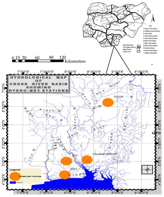
Figure 1.
Hydrological map of the Cross River Basin showing the hydromet stations (Cross River Basin Development Authority).

Table 1.
Basic information on the weather stations in the basin.
The Eket hydro station is sited in Eket local government area (LGA), which is one of the 31 local government areas in Akwa Ibom State. Eket LGA lies within latitudes 7°55 N and 8°00 N and longitudes 4°35 E and 4°40 E [49]. It is industrial city and a hub for the oil and gas industry, with so many companies providing support services for the exploration of hydrocarbons. Eket is also known for palm oil production, with the vegetation mostly populated with palm trees. The area is generally flat, with some marshy river-washed soils around the banks of the Qua Iboe River. It is located at the southern end of Akwa Ibom State and near the Atlantic Ocean, approximately 30 km southeast of Uyo, the state capital. The area covers a land area of approximately 1075 km2. It is part of the coastal plain that is characteristic of the Niger Delta and laden with wetlands, many streams, and mangrove forests. It has a low topography with an average elevation of 30 m above mean sea level (msl). The geology of the area comprises the Benin and Agbada formations [50]. The former consists of coastal plain sands, while the latter is made up of sedimentary hydrocarbon-bearing rock layers (sandstone, shale, and clay deposits). The soil is predominantly sandy, with coastal plain sands being the most common type. The land use involves subsistence farming, fishing, and hunting, with some areas also used for palm oil cultivation and tourism.
The Uyo hydro station is sited in Uyo local government area (LGA), Akwa Ibom State. Uyo LGA is located within the bounds of latitudes 5°05 N and 5°09 N and longitudes 7°41 E and 8°10 E [51]. The geology of Uyo is similar to Eket; however, it consists of the Benin formation (comprising coastal plain sands) underlain by a paralic form of the Agbada formation characterized by inter-fringing sediments from continental and marine origins [51,52]. This part of the formation is not hydrocarbon-bearing. Unlike Eket, Uyo is an inland area and is located centrally within the state. It is higher in topography than Eket, having an average elevation of 50 m. The topography is also undulating, with prominent deep ravines with slopes up to 6°8′ in some areas [53]. Uyo covers an approximate area of 188.024 km2, with an estimated population of 305,961. It was a district headquarters during the colonial era and was later upgraded to a local government headquarters. In 1987, it was further upgraded to the status of a state capital. Land use is mostly residential with decreasing vegetated areas due to the recent upsurge in economic activities [54].
Temperature regimes of Uyo correspond with that of the tropical humid climate and ranges between 26.2 °C and 35 °C, with mean annual temperature of 28.4 °C [55]. Uyo is characterized by a gentle, undulating terrain. According to [56], sandstone hills and ravine are attributed to parts of Uruan and Uyo local government areas, while other sections of the study area are filled with low-lying, undulating sandy plains terrain. The area is a low-lying terrain and is susceptible to flooding from extreme rainfall. Uyo is mainly drained by the Iba Oku stream network, which flows northwards into Ikpa River at the middle segment and empties into the Cross River Estuary. The Iba Oku drainage system drains settlements, including Anua, Eniong, Ewet, Afaha Oku, Ikot Ntuen Oku, Ndueotong and Iba Oku, and so forth. Agricultural and urban land uses are the most common found in the area. For agriculture, intensive farming without fallowing is commonly practiced in the urban and suburban areas. Urban land use includes built-up areas for various purposes. This, however, covers over 75% percent of the city and therefore suggests a clustered or high concentration of human population in the area. Intensive urban development and integrated drainage systems have rendered the surface impervious to infiltration, thereby increasing the volume of surface runoff. Besides, the urban drainage system in Uyo is channeled into the Iba Oku stream at Afaha Oku. Flooding has been a major problem affecting most parts of the study area.
Calabar and Ogoja hydro stations are both situated in Cross River State, Nigeria, adjoining Akwa Ibom State. The Calabar hydro station is in Calabar LGA, which lies between longitudes 8°15 E and 8°25 E and latitudes 4°50 N and 5°06 N [57]. Based on Köppen’s climatic classification, the area falls within the tropical rainforest climate. The original vegetation of the entire Calabar River catchment was tropical rainforest. However, most of the original vegetation in the study area has been replaced by agricultural, road construction, tree logging, and industrial and residential activities. Though the catchment can still be classified as tropical rainforest, this is clearly observed only in a few locations [58]. The Calabar metropolis is sandwiched between the Great Kwa River to the east and the Calabar River to the west. The urban area is at the eastern bank of Calabar River. Urban development of the southern part is hindered by the mangrove swamps.
Calabar covers an estimated land area of 274.593 km2. There is a shift in land use toward the northern part of the city, with built-up areas increasing at the expense of agricultural land. The topography is characterized by a mostly flat landscape with valleys, creeks, and swamps, influenced by the Atlantic Ocean and Cross River. The dominant soil type in the Calabar area, specifically in the Odukpani area of Cross River State, is shale soil, with coastal and wetland soils being predominantly sandy. The subsurface geology comprises Benin, Agbada, and Akata formations, which are covered by quaternary deposits. The Benin formation share the same characteristics as in Eket and Uyo LGAs, consisting mostly of different types of sands with interspatial deposits of clay and silt. Calabar is a coastal area and, as such, has a low-lying topography with elevations that are generally below 100 m but hilly [58]. The elevation can be as low as 10 m toward the south of the region [59]. The hills are the sources of the streams, and flow is generally in the NW-SE direction with drainage facilitated at the western part of the region by the Calabar River and to the east by the Aka River [58].
Ogoja station is in Ogoja LGA, which lies between longitudes 8°25 E and 9°00 E and latitudes 6°20 N and 6°45 N [60]. Ogoja is in the northern part of Cross River State and about 300 km from Calabar. The land use is primarily focused on subsistence agriculture, with crops like yams, cassava, and rice being cultivated, along with fishing and hunting. The soils around Ogoja station, Nigeria, are primarily alfisols and inceptisols, with some areas featuring utisols, which are derived from diverse parent rocks like sandstone, shale, and basalt. The soils are well drained with few poorly drained soils (loamy sand to sandy clay). The vegetation is characterized as forest–grassland–savanna (transitional vegetation type).
The geology of Ogoja is composed of a basement complex overlain by a sedimentary formation (Figure 2). The sedimentary formation comprises the Asu River Group (composed of shales and pyroclastics interbedded with sandstone and siltstone) directly overlying the basement complex and overlain by the Eze–Aku Group, consisting of shales with intercalations of sandstones [61,62].
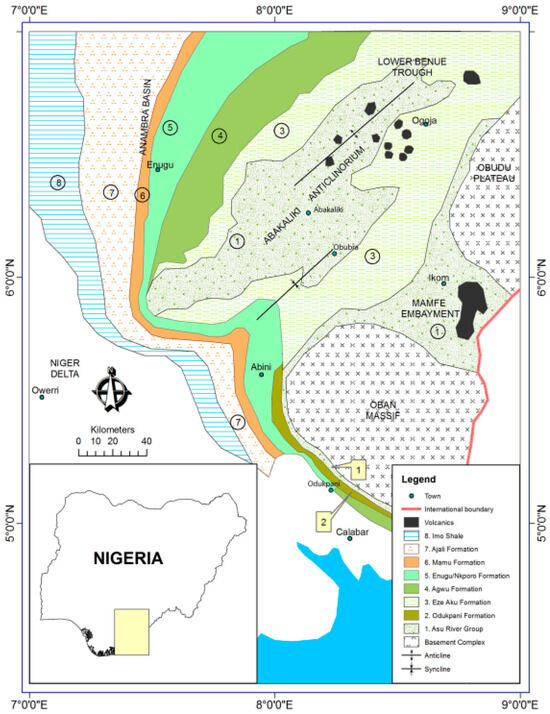
Figure 2.
Description of the geology of the Cross River Basin (From [63] N).
2.2. Methodology
The long-term effect of climate change on runoff was quantified by a climate-flood model developed based on a multiple linear regression model. Hydro-meteorological data (annual average rainfall, maximum and minimum temperatures, humidity, duration of sunlight (sunshine hours), evaporation, wind speed, soil temperature, cloud cover, solar radiation, and atmospheric pressure) for 30 years from 1992 to 2021 in four stations in the Cross River Basin were obtained from Nigerian Metrological Agency (NIMET), Abuja. To address missing data and data inconsistencies, data quality assessment was carried out by applying metadata inspection to identify visible changing points. Time series graphs were plotted on a linear scale and inspected for inconsistencies, which were screened out. Microsoft Excel was used to carry out the data quality assessment.
The selected climatic parameters used in the investigation represent the key factors that affect river discharge and runoff. These are essential climatic variables that are commonly measured at gauges and weather stations and used either singularly or jointly to describe the climatic condition of a given area and to investigate, for instance, the impact of climatic factors on agriculture (e.g., [64]) and on the flow characteristics in watersheds (e.g., [30]).
2.2.1. Multiple Linear Regression Model
Multiple linear regression, an extension of linear regression [65], is a statistical method used for modeling the linear relationship between a target variable and one or more independent explanatory variables, otherwise known as predictors. It is a type of regression analysis where the aim is to model the relationship between multiple predictors and a target, with the purpose of making predictions about the target based on new data of the predictors. Multiple linear regression determines the values of the coefficients that best fit the data, in the sense that they minimize the residual sum of squares (the difference between the observed values and the predicted values).
However, it is important to keep in mind that multiple linear regression assumes that the relationship between the target variable and explanatory variables is linear and that there is no multicollinearity between the predictors.
Montgomery and Runger [66] define a multiple regression model as shown in Equation (1):
where represents the dependent or predicted variable and is the y-intercept, i.e., the value of when and is 0. and are the regression (slope) coefficients representing the change in y in relation to a unit change in and respectively. That means that is the slope coefficient for each independent variable, . is the model random error (residual) term. and are the explanatory variables (regressors) for the ith observation.
Assuming that n observations of the variables and … are available, which are indexed by i, where i is given as 1,n. then the n realizations of the interactions can be written in matrix form, as shown in Equation (2).
εi ~iid N(0, 2), , , … are the residuals for all observations such that represents the residual for the ith observation. Each error term is a function of both the response variable and explanatory variable for that data point. If these values are IID, then this means that the deviations from the conditional mean are independent and identically distributed. The term , therefore, implies that is distributed identically and independently according to a normal distribution, with mean 0 and variance . β0 is the intercept (multi-dimensionally), β1, β2, … βk−1 are the regression coefficients for the explanatory variables, and gives the kth explanatory variable value for the ith case.
In matrix form, the multiple linear regression model for multiple observations is given as Equation (3).
and are matrices, is an () matrix, and is a () matrix. Thus, the matrices corresponding to each variable in Equation (3) are given as the
Dependent Variable matrix, and the Design matrix, X (Equation (4))
The Coefficient matrix, β and Residual matrix, are
Considering the case of only two dependent variables as it agrees with the nature of the data, Equation (1) reduces to Equation (6).
The dependent variable is the estimated monthly runoff, Y. According to Montgomery and Runger [66], are estimates of the true parameters of the regression equation. is the mean change for Y when there is a unit increase in X1 while holding X2 constant (partial regression coefficient).
2.2.2. Assumptions of the Multiple Linear Regression Model
The first assumption regarding the errors is that they have an expected value of 0
where is the error term or disturbance, the error between the observed and what the model predicts. This model describes the relation between Xi and Yi using an intercept and a slope parameter, as in Equation (1).
It is assumed that the errors are mutually uncorrelated and that they have a common variance. or, equivalently, where I is the unit matrix.
E is the error term, which is also known as the residual, disturbance, or remainder term, and is variously represented in models by the letters e, ε, or u.
σ2 is the variance.
The concept of homoscedasticity is generally referred to as “same variance” and is an important concept in linear regression because it describes how the error term (the noise or disturbance between independent and dependent variables) is the same all through the values of the independent variables.
2.2.3. Least Squares Estimation
According to Montgomery and Runger [66], the coefficient selected by least squares factor is termed the least squares predictions of the correlation variables (Equation (1)). The coefficients are comparable in the form that they generate predicted (fitted) average responses, the sum of which would be as low as possible.
The residuals are the errors in the model and are derived as the differences between the predicted and measured values.
Based on Equation (3), the multiple linear regression model for a range of observations can be rewritten as follows:
where is the vector of random errors, also known as the notation for the residual matrix. Similarly, is measured as the difference between the measured and the predicted values.
The least squares function in matrix notation is then given as
The identity is used, which comes from the fact that the transpose of a scalar, which may be constructed as a matrix of order 1 × 1, is the scalar itself. Equations (11) and (12) then become the following:
In order to minimize L with respect to , 1, and 2, the least squares estimates of , 1, and 2 must satisfy the following condition:
The first-order conditions for optimization are calculated by differentiating the function with respect to the β vector and by limiting that outcome to 0 (Equation (14)). The formulation has an exact solution and is the vector of ordinary least squares estimator, .
The vector of the least squares estimators, (estimates of , 1, and 2,), is given as the solution to Equation (14) and expressed below:
where
2.2.4. Formulation of Climate-Flood Model
The climate-flood model was formulated using discharge Q at the gauging stations as a function of measured climatic variables. The variables include annual rainfall depth R (mm), evaporation, E (mL), solar radiation, SR (w/m2), sunshine hours, SH (hours), maximum and minimum temperatures, T (C), relative humidity, RH (%), wind speed, W (Knots), soil temperature, Ts (C), cloud cover, C (oktas), atmospheric pressure, P (millibars), runoff, and Q (m3/s) for the Cross River Basin. The formulation was achieved with the observed discharge at each of the stations as a function of the various climatic variables at each station (e.g., [30]) as follows:
The values of input variables of the climate-flood model of the four stations in the basin were substituted into Equation (20). The climate parameters used were all yearly averages, which include hydro-meteorological data for annual average rainfall, maximum temperature, humidity, duration of sunlight (sunshine hours), evaporation, wind speed, soil temperature, solar radiation, and atmospheric pressure, from four stations (Eket, Calabar, Uyo, and Ogoja) in the Cross River Basin.
2.2.5. Calibration of Climate-Flood Model
In ensuring that the assumptions of the multiple linear regression model as shown in Equations (7)–(9) were achieved, the logarithm to base 10 of the left-hand side (LHS) and right-hand side (RHS) of Equation (20) was applied to linearize the function as shown in Equation (21).
Additionally, the R statistical software (Version 4.3.1) was used to estimate the least squares estimates of the regression parameters.
From our first round of data analysis, contributions from cloud cover (C) were insignificant; therefore, the cloud cover parameter was eliminated, giving rise to Equation (22) below:
If the logarithmic term on the left-hand side in Equation (22) is substituted by the dependent (predicted) variable of Equation (1), , and each logarithmic term on the right-hand side in Equation (22) is substituted by regressor (independent) variables (), Equation (22) is transformed to Equation (23).
That is,
To obtain () using the least squares method [67,68], Equation (24) is transformed into its matrix form. The least squares estimate of the regression parameters, is then calculated from Equation (19). After the coefficients are determined, they are substituted in Equation (22). The climate-flood model, which in this case is the regression model, is used to forecast the annual runoff for each catchment under investigation. Data for the predictors were taken as the annual records of the climatic variables from each of the four gauge stations (Calabar, Ogoja, Uyo, and Eket). It is crucial to note that Equation (22) only provides the runoff generated by the climatic variables studied in this work and does not consider other factors such as soil saturation, human activities, land use, and drainage systems.
3. Results and Discussion
3.1. Climate-Flood Model for Calabar
The estimates of regression coefficients were substituted in Equation (20) to obtain the fitted climate-flood model of the Calabar River, given as
where R is rainfall, S is sunshine hours, T is temperature, E is evaporation, RH is relative humidity, SR is solar radiation, Ts is soil temperature, and W is wind speed.
Q = 0.2590R1.000S−0.001T0.002E−0.001RH−0.004SR−0.0020TS−0.001W0.001
The parameter estimates of the model specified for the Calabar River are given in Table 2, along with their standard error and 95% confidence intervals. Based on the information in the table and Equation (25), the regression coefficient for annual rainfall depth has the highest estimated value of 1.000. Our model, therefore, indicates that among the climatic parameters, only annual rainfall has a significant impact on runoff at 95% confidence intervals in the Calabar River Basin. It also shows that as rainfall increases, runoff increases. Additionally, the model indicates that a change in evaporation by a value −0.001, sunshine hours by a value of −0.001, relative humidity by a value of −0.004, solar radiation by a value of −0.002, and soil temperature by a value of −0.001 leads to significant increases in runoff/flows/discharge in the Calabar River.
Table 2.
Parameter estimates with associated standard errors and confidence intervals for Calabar station.
Table 3 explains the adequacy of the model for the Calabar station, with an R2 value of 1.000, meaning the model was able to explain 100% of the variation in the dependent variable.
Table 3.
Analysis of variance (ANOVA) for the regression model for Calabar station.
The study of the Cross River Basin also revealed that climatic variables accounted for 100% of the yearly changes in runoff. This shows that the climate has a major impact on runoff and flooding in Calabar and that changes in climate can lead to changes in runoff and flooding.
The ANOVA table is used to assess the model adequacy of a multiple regression analysis. In this context, it helps to determine whether the regression model is a good fit for the data and whether the independent variables collectively explain a significant amount of the variance in the dependent variable. The ANOVA table is explained as follows:
- Source: This column indicates the sources of variance in the analysis. In a typical ANOVA table for regression, you will usually find three sources:
- (a)
- Model: This source represents the variance explained by the regression model, which includes all the independent variables. In Table 3, the sum of squares of the variabilities is given as 3782.633.
- (b)
- Residual: This source represents the unexplained or error variance. It is the variance that the model does not account for, and it includes random noise in the data. This is given as 0.000127 in Table 3 for the sum of squares of the variabilities.
- (c)
- Uncorrected Total: This is the total variance in the dependent variable before any modeling. It is the sum of the model and residual sources, which is 3782.633 in Table 3 for the sum of squares of the variabilities.
- Sum of Squares (SS): This is a measure of the variation of the independent variables, which is crucial because of the impact these have on the trend of the dependent variable.
- Degrees of Freedom (DF): DF indicates the number of degrees of freedom associated with each source. In regression analysis, the DF for the model is typically the number of independent variables (including the intercept) minus 1, and the DF for residual is the total number of data points minus the number of parameters in the model. In Table 3, DF for the model is 10, DF for the residuals is 14, and the uncorrected total is 24.
- Mean Squares (MS): Mean squares are obtained by dividing the sum of squares by the degrees of freedom. It represents the variance explained or unexplained per degrees of freedom. In Table 3, MS is 378.263 (3782.633/10) for the model, and MS is 9.07143 × 10⁻⁶ (0.000127/14) for the residuals.
- R2 (R-squared): R2, often called the coefficient of determination, represents the proportion of variance in the dependent variable that is explained by the independent variables in the model. In Table 3, R2 is 1.0, which means that approximately 100% of the variance in the dependent variable is explained by the independent variables.
Interpretation:
The high R2 value (1.0) suggests that the regression model is a very good fit for the data. It explains almost 100% of the variance in the dependent variable.
The model’s sum of squares (3782.633) is much larger than the residual sum of squares (0.000127), indicating that the model explains a significant amount of the variance in the dependent variable.
The F-statistic can be calculated by dividing the model MS by the residual MS. If the F-statistic is significantly larger than 1, it suggests that the model is a good fit for the data. You would typically perform a hypothesis test using the F-statistic to determine if the model is statistically significant.
In summary, this ANOVA table provides evidence that the regression model is a good fit for the data and that the independent variables have a significant impact on explaining the variance in the dependent variable.
The R-squared (R2) value, which represents the proportion of variance in the dependent variable explained by the independent variables in a regression model, is computed using the values from the ANOVA table (Table 3). From Table 3, R2 is given as 1.000, which indicates that approximately 100% of the variance in the dependent variable is explained by the independent variables in the model.
R2 can be calculated manually as the ratio of the model sum of squares (SS) to the uncorrected total sum of squares (SS).
R2 = Model SS/Uncorrected Total SS
From the ANOVA table, model SS is 3782.633, uncorrected total is 3782.633, and R2 is 3782.633/3782.633 ≈ 1.000. This matches the value in the ANOVA table and means that approximately 100% of the variance in the dependent variable is explained by the independent variables in the multiple regression model.
Values of the coefficient of determination R2 are given at the bottom of each ANOVA table. These were determined at a 5% significance level (p = 0.05). The p-value for all tests is lower than 0.05, suggesting that the observed results, including the F-statistic, are unlikely to have occurred by chance.
3.2. Climate-Flood Model for Uyo
The estimates of regression coefficients were substituted into Equation (20) to obtain the fitted climate-flood model of the Uyo River as
Q = 0.263R0.995S0.002T−0.069E−0.011RH0.018SR−0.011Ts0.011W0.001
The strongest predictor of runoff variability in the Uyo region, as revealed by the climate-flood model (Equation (27)), is rainfall with a value of 0.995. The parameter estimates of the model specified for the Uyo River, presented in Table 4, include their standard errors at 95% confidence intervals. This result implies that as rainfall increases, runoff also increases. Furthermore, the table shows that as temperature, evaporation, and solar radiation decreases, there is a significant increase in runoff. A decrease in evaporation, indicated by a value of −0.011, predicts an increase in runoff in Uyo.
Table 4.
Parameter estimates with associated standard errors and confidence intervals for Uyo station.
The model’s ability to explain the variation in the dependent variable for the Uyo River is shown in Table 5 with an R2 value of 1.000. This means that the model was successful in explaining 100% of the variation.
Table 5.
Analysis of variance (ANOVA) for the regression model for Uyo station.
Furthermore, the results of the study of the Uyo station showed that the climatic variables accounted for 100% of the annual variation in runoff. This indicates that a change in the climate conditions influences runoff and flooding in Uyo.
3.3. Climate-Flood Model for Ogoja
The estimates of regression coefficients were substituted into Equation (20) to obtain the fitted climate-flood model of the Ogoja River as
Q = 0.0040R0.896S0.506T−1.571E0.371RH0.503SR−0.530Ts0.788W0.087
According to the climate-flood model for Ogoja (Equation (28) and Table 6), rainfall depth, with a value of 0.896, is the most significant climatic variable in predicting the variability of runoff for Ogoja. In this study, the parameter estimates for the model specified for the Ogoja station, as presented in Table 6, were calculated with standard errors at 95% confidence intervals. The most significant predictor of increased flooding in Ogoja is the increase in rainfall depth. According to the analysis, a decrease in temperature with a value of −1.571 and solar radiation with a value of −0.530 increases runoff in this station.
Table 6.
Parameter estimates with associated standard errors and confidence intervals for Ogoja station.
As shown in Table 7, the results of the study of the Ogoja station revealed that climatic variables accounted for 98.8% of the yearly changes in runoff, while non-climatic variables accounted for only 1.2%. This shows that the climate has a significant impact on runoff and flooding in Ogoja.
Table 7.
Analysis of variance (ANOVA) for the regression model for Ogoja station.
3.4. Climate-Flood Model for Eket
The estimates of regression coefficients were substituted into Equation (20) to obtain the fitted climate-flood model of the Eket River as
Q = 0.052R0.988S0.0001T−0.308E−0.041RH−0.031SR−0.049Ts0.063W0.018
The climate-flood model for Eket (Equation (29) and Table 8) indicates that rainfall, with a value of 0.988, is the dominant factor in determining runoff variability. The parameter estimates of the Eket station model, with standard error at 95% confidence intervals, demonstrate that an increase in rainfall leads to a corresponding increase in flooding. The study also found that a decrease in evaporation, with a value of −0.041 and temperature with a value of −0.308, has a significant effect on increasing runoff in Eket. Additionally, relative humidity and solar radiation were found to play a significant role in influencing runoff in the Eket region.
Table 8.
Parameter estimates with associated standard errors and confidence intervals for Eket station.
The results of the study of the Eket station (Table 9) indicate that the climatic variables accounted for 99.9% of the annual variation in runoff, whereas the non-climatic variables accounted for 0.1%. This demonstrates that the climate influences runoff and flooding in Eket.
Table 9.
Analysis of variance (ANOVA) for the regression model for Eket station.
In summary, the model output in this study suggests that changes in climate have an impact on the runoff and flooding. This aligns with the results from Babatola and Akinnnubi [41], where 54.4% of the annual runoff variation in River Niger was attributed to climatic factors. This is also in line with the previous studies of Ekwueme and Agunwamba [30] on the influence of meteorological variables on runoff in a tropical watershed, where climatic variables accounted for 66.1% of the runoff variation in Adada River.
The effect of precipitation (rainfall) on flow in catchments is so large because, from the analyzed models, precipitation has the most significant impact on flow/runoff. For instance, from the analysis for Calabar station, the regression coefficient for annual rainfall depth has the highest estimated value of 1.000. The model, therefore, indicates that among the climatic parameters, only annual rainfall has a significant impact on runoff at 95% confidence intervals in the Calabar River station. It also shows that as rainfall increases, runoff increases.
From the climate flood model, a rise in temperature reduces runoff by a factor of −0.069 in Uyo station. In Eket, increases in temperature reduce runoff/flooding by a factor of −0.308 and, in Ogoja, reduce runoff by −1.571. It is only in Calabar that the reverse is the case, with a factor of 0.002. However, this value is trivial and is considered to have negligible impact on runoff. It is insignificant in comparison to the effect of rainfall in the Calabar catchment area. The implication of this investigation is that changes in rainfall believed to be governed by climate change are the major determinant of flooding in the entire study area.
3.5. Multicollinearity Test for Model Adequacy
Multicollinearity is a statistical phenomenon that happens when there is a strong correlation between two or more independent variables in a regression model. That is, multicollinearity shows whether the predictor variables have a strong linear relationship. If there is collinearity, it may be difficult to precisely ascertain the unique effects of each independent variable on the dependent variable when performing a regression analysis. It may be challenging to interpret the findings and derive meaningful inferences from the model due to unstable and incorrect estimations of coefficients because of multicollinearity.
For regression models to be reliable and valid, multicollinearity must be identified and resolved. Multicollinearity occurs when two or more independent variables in a data frame have a strong association with one another in a regression model [69].
VIF are the variance inflation factors. The strength of correlation between the independent variables is assessed using VIF. By regressing a variable against every other variable, VIF is predicted. It measures how much collinearity has inflated the variance (or standard error) of the calculated regression coefficient. The variance inflation factor is expressed as , where R2 is the coefficient of determination.
Examining the range of R2 (0 ≤ R2 ≤ 1), R2 = 0 implies that the model is unable to explain the variance in the dependent variable, while R2 = 1 suggests the opposite. That is, the model explains the variance in the dependent variable. In other words, there is goodness of fit.
3.5.1. Multicollinearity Test for Uyo Station
Table 10 above presents the multiple linear regression analysis results for Uyo for test of multicollinearity using all the variables. From the analysis (Table 10), the VIF values are all less than 5. This shows that there is no multicollinearity problem in the variables at Uyo station.
Table 10.
Multiple linear regression analysis results for Uyo using all the variables.
3.5.2. Multicollinearity Test for Calabar Station
Table 11 above presents the multiple linear regression analysis results for Calabar station for test of multicollinearity using all the variables. From the analysis (Table 11), the VIF values are all less than 5. This shows that there is no multicollinearity problem in the variables at Calabar station.
Table 11.
Multiple linear regression analysis results for Calabar station using all the variables.
3.5.3. Multicollinearity Test for Eket Station
Table 12 above presents the multiple linear regression analysis results for Eket station for test of multicollinearity using all the variables. From the analysis (Table 12), the VIF values are all less than 5. This shows that there is no multicollinearity problem in the variables at Eket station.
Table 12.
Multiple linear regression analysis results for Eket using all the variables.
3.5.4. Multicollinearity Test for Ogoja
Table 13 represents the multicollinearity test for the linear regression model for Ogoja station. From our results, a unit increase in rainfall will result in the same quantity of runoff. Increase in rainfall by 0.0030 produces runoff and flooding by a value equal to 0.0030 in Ogoja, given that R2 = 1.00 in Ogoja. Rainfall and maximum temperature with VIF (variance inflation factors) greater than 5 are the parameters we can eliminate in Ogoja because of multicollinearity. The model’s assumption of the problem of multicollinearity in the entire Cross River Basin catchment is only in Ogoja station, although it does not invalidate the model.
Table 13.
Multiple linear regression analysis results for Ogoja using all the variables.
To overcome the effect of multicollinearity in Ogoja station, a multiple linear regression analysis was carried out using composite variables (variables that did not show multicollinearity, e.g., minimum temperature, solar radiation, sunshine hours, relative humidity, wind speed, soil temperature, and evaporation) (Table 14 and Table 15). This is similar to the approach adopted by Chinelo and Ozlem [70], where the effect of multicollinearity on climate variables was investigated. In their work, the result of the multiple linear regression analysis revealed a strong effect of multicollinearity among the variables used with VIF > 5. To overcome this effect of multicollinearity, a principal component regression analysis was introduced. The result obtained from the principal component regression analysis of the retained variables yielded a preferable result with a VIF value of 1.039, which was much lower in comparison to when all the variables were applied.
Table 14.
Multiple linear regression analysis results excluding variables with VIF > 5 for Ogoja.
Table 15.
Predicted and observed runoff between 2016 and 2021, inclusive, at the gauge stations of Cross River Basin: (a) Discharge rates at Calabar, (b) Discharge rates at Eket, (c) Discharge rates at Uyo, (d) Discharge rates at Ogoja.
Table 14 is the multiple linear regression analysis results for Ogoja station, excluding variables with VIF > 5. In this analysis, rainfall and maximum temperature are isolated to account for multicollinearity. By eliminating rainfall and maximum temperature, R2 reduces to 0.597. This implies a reduction in the model adequacy.
In Figure 3a, standardized coefficients were used to plot the feature importance for Calabar station using all the variables. The VIF values indicate no multicollinearity. In Figure 3b, standardized coefficients were used to plot the feature importance for Eket station using all the variables. There is no multicollinearity in Eket station based on the VIF values. In Figure 3c, standardized coefficients were used to plot the feature importance for Uyo station using all the variables. There is no multicollinearity in Uyo station based on the VIF values. Likewise, in Figure 3d, the standard coefficients were used to plot the feature importance for Ogoja station using all the variables. The multicollinearity assumption failed in Ogoja station based on the VIFs.
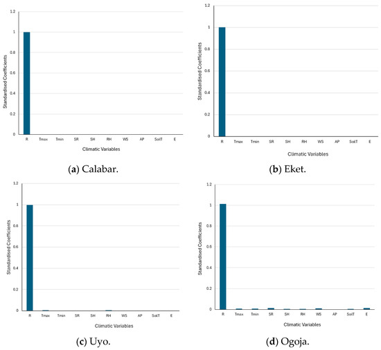
Figure 3.
Feature importance of all variables for the regions within the Cross River basin: (a) Feature importance of all variables for Calabar, (b) Feature importance of all variables for Eket, (c) Feature importance of all variables for Uyo, (d) Feature importance of all variables for Ogoja.
For Ogoja, there is a considerable change in the feature importance when all variables with VIF > 5.0 are excluded (Figure 4), indicating an increase in dominance of variables that were previously less consequential.
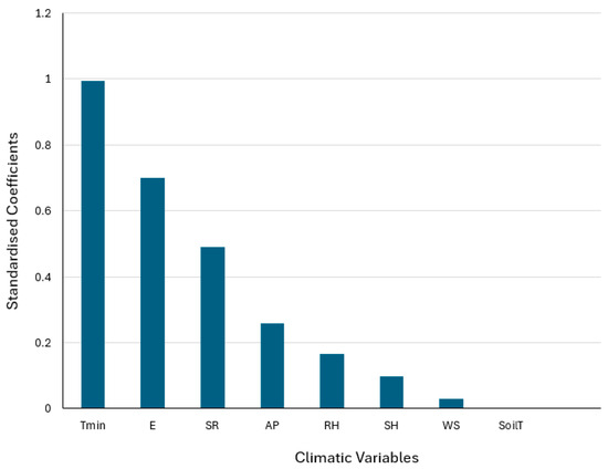
Figure 4.
Feature importance for Ogoja, excluding the variables with VIF > 5.
3.6. Model Validation
As mentioned in Section 3.1, the coefficient of determination, R2, is a measure of the portion of variance in the runoff that is explained by the predictor (climatic) variables incorporated in the models. High R2 values are recorded based on the ANOVAs, which is an indication of the extent of the collective influence of the climatic variables on streamflow (channel runoff). The set of high R2 values also shows that the flood models are a good fit for the recorded data, with minimal impingement from other factors outside the boundaries of the model. Large magnitudes of R2 and R for calibrated and validated flood models are indications of the high precision in their ability to reproduce and/or predict discharge values. High values of R2 and R, above 0.900, which denote the accuracy of flood models, are realizable. These have been achieved by others while constructing other flood models, as shown for instance by Addison-Atkinson et al. [71] and Zarei et al. [72]. The former evaluated the performance of flood models by simulating surface flood events, including surface runoff, and their interactions with underground sewer flow systems, while the latter compared the capabilities of the Hydrologic Engineering Center’s Hydrologic Modelling System (HEC–HMS) used in conjunction with machine learning models. On one hand, HEC–HMS was combined with a long short-term memory (LSTM) network model (HEC–HMS–LSTM), while on the other hand, it was linked with a gated recurrent unit (GRU) model (HEC–HMS–GRU). Both hybrid models were used to examine the effect of climate change on flood events.
Whereas R2 shows the percentage of the overall variance described by the regression model (including how much of the linear variation in the observed values is explained by the variation in the projected values) [73], model validation is a vital stage in assessing its performance on unseen data to ensure its reliability and accuracy. One of the most popular methods for assessing the accuracy of model predictions is the scatter plot of predicted versus observed (or vice versa) values. Indices for evaluating—and increasing confidence in—model performance are provided through the slope and the intercept of the line fitted to the data. The slope and intercept reflect the consistency and the model bias. An alternative approach is to determine the coefficient of correlation (R), which is an indicator of the intensity and direction of the linear relationship between the predicted and observed values. R ranges from −1 to +1. Values closer to |1| suggest a strong correlation between two variables. Positive values imply a direct and linear relationship and vice versa for negative values. The concept of R is adopted herein to test the validity of the models developed in this study.
In total, 80% of the data (1992–2015) were used to train the models and were therefore not used in the main validation process. Model validation was carried out using 20% of the dataset (2016–2021). The four models were tested by comparing the observed discharge flows with those predicted within the same time frame (2016–2021). Coefficients of correlation were calculated at 95% confidence intervals (p = 0.05) (Table 15 and Figure 5). The high correlation coefficient (R) is an indication of how close the predicted and observed flows are.
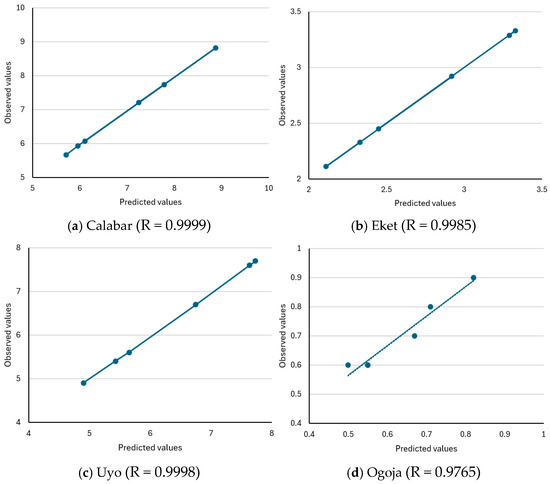
Figure 5.
Plot of predicted versus observed values for all stations. (a) Predicted versus observed flows for Calabar and the coefficient of correlation (R = 0.9999), (b) Predicted versus observed flows for Eket and the coefficient of correlation (R = 0.9985), (c) Predicted versus observed flows for Uyo and the coefficient of correlation (R = 0.9998), (d) Predicted versus observed flows for Ogoja and the coefficient of correlation (R = 0.9765).
A visual inspection of the scatter plots is also necessary. From Figure 5a, the prediction of the multiple linear regression model (climate-flood model) for Calabar (Equation (25)) is accurate because almost all the points are in a straight line. The closer the points to the straight line, the more accurate the prediction is. Predicted values are the runoff predicted using the model (Equation (25)). Equation (25) and Figure 5a, therefore, confirm that an increase in rainfall depth increases runoff by a value of 1.000 in Calabar station and its environs. Figure 5b shows that the prediction of our multiple linear regression model (climate-flood model) for Eket station (Equation (29)) is accurate because almost all the points are on the straight line. The closer the points are to the straight line, the more accurate the prediction is. The predicted values are those determined by the model. The same pattern is depicted in Figure 5c, which is the plot of residuals versus predicted values for Uyo station. The points are in a straight line, indicating that the model (Equation (27)) fit is adequate. Figure 5d shows a slight disparity between the predicted and observed values for Ogoja, as indicated by the offsets of the data points. This does not undermine the accuracy of the model (Equation (28)) since the differences between the predicted and observed values, as shown in Table 15, are trivial.
In addition, a set of one-way ANOVA was included to complement the model validation process (Table 16, Table 17, Table 18 and Table 19). These were conducted using the predicted and observed runoff values from 2016 to 2021 (Table 15). Results for the four catchment areas are given in Table 16, Table 17, Table 18 and Table 19. In this context, ANOVA serves as a way of assessing the fitness of the model to the observed unseen data and to determine if the differences or similarities are statistically significant. The F-statistic values for all gauge stations are many folds larger than 1, which suggests that the model results closely match the observed unseen data. In other words, the model can reproduce the observed data with minimal errors. At a 95% confidence interval (significance level, = 0.05), DF = 1, and DF = 4, the critical F-value is 7.71. The calculated F-statistic values for all gauge stations are greater than the critical value. Therefore, at the 0.05% significant level, there is no difference between the predicted and observed values.
Table 16.
One-way ANOVA results comparing observed and predicted values for Calabar station.
Table 17.
One-way ANOVA results comparing observed and predicted values for Uyo station.
Table 18.
One-way ANOVA results comparing observed and predicted values for Ogoja station.
Table 19.
One-way ANOVA results comparing observed and predicted values for Eket station.
In summary, multicollinearity tests were used to check the presence of any significant correlation between the predictor variables used in the model. In this case, the variance inflation factor (VIF) is used as an indicator. A VIF greater than 5 is considered large enough to suggest collinearity between predictor variables, while a VIF less than 5 indicates the contrary. Multicollinearity was only observed in Ogoja station; however, this did not compromise the accuracy of the model built with the climatic variables from that station.
There may be a relationship between sunshine hours and solar radiation and evaporation and temperature or sunshine hours, but these are not considered high enough to affect the measurements of their unique effects on the dependent variable when performing the regression analysis. Other forms of correlation analysis were not included because it is considered outside the scope of this article. This is recommended for future investigations, which will include correlation analyses to determine the strength of association between predictor climatic variables.
The primary aim of the study is to investigate the impact of climatic variables on runoff flow over a given time frame, which was carried out using a 30-year data set. The models have been verified for goodness of fit and checked against multicollinearity. To verify the model, its performance was evaluated using the coefficient of determination as an indicator to determine the extent to which the variance in the dependent variable is accounted for by the predictor variables. The model validation was successful, wherein predicted values were shown to match actual values observed at all hydro stations (Ogoja, Uyo, Calabar, and Eket).
3.7. Summary of Model Findings and Implications
The least squares estimate of the regression parameters, , are calculated from Equation (19). After finding the coefficients, they are substituted back into the original equation (Equation (22)) to determine the regression model, also referred to as the climate-flood model. The yearly runoff for each of the stations is predicted with the climate-flood model using data from the average annual climatic variables for each of the four stations as predictors. Importantly, it should be noted that Equation (22) yields runoff produced by only climatic variables as established in this work without other variables such as soil saturation, anthropogenic activities, land use, and changes in lifestyle. There are changes in climate in the catchment area, and these are impacting fluctuations in flooding at the different stations. For instance, at the Calabar station, the regression coefficient for annual rainfall depth has the highest estimated value of 1.000. Our model, therefore, indicates that among the climatic parameters, only annual rainfall has a significant impact on runoff at 95% confidence intervals in the Calabar River basin. It also shows that as rainfall increases, runoff increases.
Following our analysis, a new set of climate-flood models (Equations (25) and (27)–(29)) were developed for Calabar, Ogoja, Uyo, and Eket, which is a fair representation of the catchment of Cross River Basin (Akwa Ibom State and Cross River State). The findings suggest that at 95% confidence interval, the climate-flood model was effective in forecasting the annual runoff at all the stations. The findings also identified the climatic parameters that were responsible for 100% of the runoff variability in Calabar (R2 = 1.000), 100% of the runoff in Uyo (R2 = 1.000), 98.8% of the runoff in Ogoja (R2 = 0.988), and 99% of the runoff in Eket (R2 = 0.999). From the model, annual rainfall depth is the only climate parameter that significantly predicts runoff at 95% confidence intervals in Calabar station, while in Ogoja, rainfall depth, temperature, and evaporation significantly predict runoff. In Eket, rainfall depth, relative humidity, solar radiation, and soil temperatures are significant predictors of runoff. The model also reveals that rainfall depth and evaporation are significant predictors of runoff in Uyo. The implications of the model findings are as follows:
- Calabar:
Climate parameters are responsible for 100% runoff variability in Calabar and its environs. This result agrees with the findings of Ekweme and Agunwamba [30], where climatic variables were responsible for 64.73% of annual variability of runoff at Adada River in Enugu State, Nigeria. Specifically, rainfall was modelled to be the only positive climatic parameter that significantly increases runoff. From the model in this study, a rise in rainfall increases runoff by a factor of 1.000. The implication is that changes in rainfall are the major determinant of flooding in the Calabar catchment. With respect to the impact of climate change, this study shows that a decline in rainfall will ultimately lead to less runoff and a consequent reduction in flooding in Calabar. Additionally, the model indicates that a change in sunshine hours by a value of 0.001, evaporation by a value of −0.001, relative humidity by a value of −0.004, soil temperature by a value of −0.001, and solar radiation by a value of −0.002 leads to a significant reduction in runoff.
- 2.
- Uyo:
From our results, climate parameters were responsible for 100% of the runoff variation in Uyo and its environs. This means that non-climate predictors do not contribute to runoff. It, therefore, implies that climate change has an overriding impact on flooding in Uyo. This is consistent with the findings of Babatolu and Akinnubi [41], where 54.4% of the annual runoff variation in Niger River was attributed to climatic factors. In Uyo, results from this study indicate that an increase in rainfall will increase runoff by a factor of 0.995, while reductions in temperature, evaporation, and solar radiation will increase runoff and flooding in Uyo and its environs.
- 3.
- Eket:
The climate-flood model for Eket shows that at 95% confidence interval, climatic variables account for 99.9% of runoff variation in Eket and its environs, while non-climatic factor contribute 0.1% to the runoff and flooding in the station. This aligns with the studies by Xu et al. [74], where impacts of climate change and variations in climatic variables accounted for 26.9% decrease in runoff. Due to the dynamics of climate change around Eket station, an increase in rainfall, by a factor of 0.988, contributes to the same rise in runoff and flooding, while decrease in temperature, evaporation, relative humidity, and solar radiation increases runoff/flooding by the corresponding factors of −0.308, −0.041, −0.031, and −0.049, respectively.
Findings from our validated model show that at Ogoja, climatic variables are responsible for runoff variation by 98.8%, while non-climatic factors account for 1.2%. The climatic parameters that significantly predict runoff are mainly rainfall, which increases runoff by a factor of 0.896. Decrease in solar radiation by a factor of −0.530 and temperature by −1.571 increases runoff.
The outcome of the study suggests that climate change has impacted runoff and flooding within the Cross River Basin. Average annual flow or channel runoff (streamflow) is a key component for flood hazard assessment. Although complex, there is a relationship between average annual flow and flood hazard. This is so because the average annual flow can be used to determine the probability of the occurrence of a flood event and its severity. This can be understood through concepts like the return period (recurrence interval) and the annual exceedance probability (AEP). The return period is the average time in years it takes for the reoccurrence of a flood of a given magnitude, whereas the AEP is the probability of a given magnitude of flood occurring in a specified year. Generally, a higher average annual flow increases the potential for a flood event because of the likelihood of the flow to overrun the river channel banks. When the relationship between flood frequency and average annual flow is established, the information can then be used to carry out flood risk assessment, which would help identify areas that are most vulnerable. An illustration of the application of average annual flow in flood risk assessments is shown in Ibrahim et al. [75].
This study presents protocols that can be applied to predict average annual runoff (streamflow) within the defined catchment areas, thus providing one of the vital information necessary for flood hazard identification and management. Basin-scale empirical relationships between influencing climatic parameters and flow are derived. Previous research by Agbiji et al. [76] shows that trends in climatic variables are determined by climate change. It is the assertion in this study that if climatic parameters are invariably affected by climate change, then flow will be affected as well based on the relationships that have been established. It is, hence, possible to predict fluctuations in flow, which is a useful resource in water resource planning, including flood risk management.
4. Conclusions
In this study, the influence of climate change on flooding in the Cross River Basin sub-region was modeled by examining the effects of climatic variables such as rainfall, evaporation, solar radiation, wind speed, relative humidity, and sunshine hours. The results of the study showed that these climatic variables at 95% confidence accounted for 98.8% of the annual variation in runoff in Ogoja, 99.9% in Eket, 100% in Uyo, 100% in Calabar, and subsequent flooding in the Cross River Basin. The climate-flood model of the Calabar, Uyo, Ogoja, and Eket stations proved statistically significant in predicting yearly runoff and flooding in the basin, according to the multiple regression analysis. The statistical significance results equally demonstrated that the impacts of soil temperature, relative humidity, evaporation, and temperature on yearly runoff were significant. However, because they were not statistically significant, solar radiation, sunshine hour, and wind speed had only minimal effects on annual runoff/flooding.
These findings provide valuable insights for the Presidential Panel on Climate Change, the Presidential Committee on Flooding, private investors, policymakers, civil engineers, and all other stakeholders in the water sector in developing a basin- or sub-regional-level approach to mitigating the impact of climate change. They demonstrate the potential for runoff alterations brought on by climate change that would necessitate large-scale planning responses. The study also reveals the importance of studies on floods and the hydrological effects they have on water supplies, which are crucial when weighing the costs and other implications of projected climate change.
The selected parameters represent a broad range of influencing climatic variables that are generally observed at hydro stations, and a key objective of the study was to investigate the predominance of these variables in the runoff process. The set of climatic variables used in this research have been the subject of inquiry in other related studies (e.g., [30,32,33,34,36,41,77,78]) either individually or collectively and have been shown to affect runoff to various extent, thereby forming the basis for their inclusion in this study. The outcome of this research reveals that although a number of climatic variables contribute to runoff in the designated catchment areas, rainfall is by far the most impactful. This study can be extended to cover other input parameters and catchment properties like land use, topography, infiltration, and soil type to further calibrate the climate-flood model. This is a potential area for future research.
Author Contributions
Conceptualization, N.M.A., J.C.A. and K.I.-I.I.E.; Methodology, N.M.A., J.C.A. and K.I.-I.I.E.; Software, N.M.A., J.C.A. and K.I.-I.I.E.; Validation, N.M.A. and K.I.-I.I.E.; Formal analysis, N.M.A., J.C.A. and K.I.-I.I.E.; Investigation, N.M.A. and K.I.-I.I.E.; Resources, N.M.A., J.C.A. and K.I.-I.I.E.; Data curation, N.M.A.; Writing—original draft, N.M.A.; Writing—review and editing, J.C.A. and K.I.-I.I.E.; Visualization, K.I.-I.I.E.; Supervision, J.C.A. and K.I.-I.I.E.; Project administration, J.C.A.; Funding acquisition, N.M.A. All authors have read and agreed to the published version of the manuscript.
Funding
This research received no external funding.
Data Availability Statement
Datasets for the period analysed in this study were obtained from Nigerian Meteorological Agency (NiMet). Data archiving is underway with Centre for Environmental Data Analysis (CEDA). CEDA is part of the Natural Environment Research Council (NERC) Environmental Data Service (EDS) and manages research data derived from atmospheric and earth observations.
Conflicts of Interest
The authors declare that they have no known competing financial interests or personal relationships that could have appeared to influence the work reported in this paper.
Abbreviations
| Symbol | Definition |
| ANOVA | Analysis of variance |
| CRBDA | Cross River Basin Development Authority |
| NIMET | Nigerian Meteorological Agency |
| MLR | Multiple linear regression |
| Error term | |
| Variance | |
| Q | Discharge |
| Change in discharge plus discharge | |
| R | Rainfall depth |
| S | Sunshine hours |
| T | Temperature |
| E | Evaporation |
| RH | Relative humidity |
| SR | Solar radiation |
| Ts | Soil temperature |
| W | Wind speed |
| VIF | Variance inflation factors |
| Regression coefficients | |
| R2 | Coefficient of determination |
| X1 | Composite variable based on the standardized z scores of R, Tmin, and Tmax |
| X2 | Composite variable based on the standardized z scores of Tmax and Tmin |
| X3 | Composite variable based on the standardized z scores of Tmin, Ts, and E |
| X4 | Composite variable based on the standardized z scores of SR, RH, and Ts |
| X5 | Composite variable based on the standardized z scores of SH and E |
References
- Salami, A.W.; Mohammed, A.A.; Adeyemo, J.A.; Olanlokun, O.K. Assessment of Impact of Climate Change on Runoff in the Kainji Lake Basin Using Statistical Methods. Int. J. Water Resour. Environ. Eng. 2015, 7, 7–16. [Google Scholar] [CrossRef]
- The New York Times. Nigeria Floods Kill Hundreds and Displace Over a Million. 2022. Available online: https://www.nytimes.com/2022/10/17/world/africa/nigeria-floods.html (accessed on 4 November 2023).
- Kumari, R.; Mayoor, M.; Mahapatra, S.; Parhi, P.K.; Singh, H.P. Estimation of Rainfall-Runoff Relationship and Correlation of Runoff with Infiltration Capacity and Temperature over East Singhbhum District of Jharkhand. Int. J. Eng. Adv. Technol. 2019, 9, 461. [Google Scholar] [CrossRef]
- Tofiq, F.A.; Güven, A. Potential Changes in Inflow Design Flood under Future Climate Projections for Darbandikhan. Dam. J. Hydrol. 2015, 528, 45–51. [Google Scholar] [CrossRef]
- Xu, Z.X.; Takeuchi, K.; Ishidaira, H. Monotonic Trend and Step Changes in Japanese Precipitation. J. Hydrol. 2003, 279, 1–4. [Google Scholar] [CrossRef]
- Auld, H.; Maclver, D. Changing Weather Patterns, Uncertainty and Infrastructure Risks: Emerging Adaptation Requirements. In Proceedings of the EIC Climate Change Technology, Ottawa, ON, Canada, 10–12 May 2006; IEEE: Ottawa, ON, Canada, 2006; pp. 1–10. [Google Scholar]
- Kundzewicz, Z.W. Flood Risk and Vulnerability in the Changing Climate. Ann. Wars. Univ. Life Sci.–SGGW 2008, 39, 21–31. [Google Scholar] [CrossRef]
- Parry, M.L.; Canziani, O.F.; Palutik, J.P.; van der Linden, P.J.; Hanson, C.E. Climate Change 2007: Impacts, Adaptation and Vulnerability. Contribution of Working Group II to the Fourth Assessment Report of the Intergovernmental Panel on Climate Change IPCC.; Cambridge University Press: Cambridge, UK, 2007. [Google Scholar]
- IPCC. Managing the Risks of Extreme Events and Disasters to Advance Climate Change Adaptation; Field, C.B., Barros, V., Stocker, T.F., Qin, D., Dokken, D.J., Ebi, K.L., Mastrandrea, M.D., Mach, K.J., Plattner, G.-K., Allen, S.K., et al., Eds.; Cambridge University Press: Cambridge, UK, 2012. [Google Scholar]
- Das, T.D.; Cayan, D.R.; Hidalgo, H.G. Potential Increase in Floods in Californian Sierra Nevada under Future Climate Projections. Clim. Chang. 2011, 109, 71–94. [Google Scholar] [CrossRef]
- United Nations Climate Change News. Climate Change Is an Increasing Threat to Africa. 2020. Available online: https://unfccc.int/news (accessed on 4 May 2023).
- IPCC. Climate Change 2021: The Physical Science Basis. In Working Group I Contribution to the Sixth Assessment Report of the Intergovernmental Panel on Climate Change; Masson-Delmotte, V., Zhai, P., Pirani, A., Connors, S.L., Péan, C., Chen, Y., Goldfarb, L., Gomis, M.I., Mathews, J.B.R., Berger, S., et al., Eds.; Cambridge University Press: Cambridge, UK, 2021. [Google Scholar]
- Collier, P.; Conway, G.; Venables, T. Climate Change in Africa; Oxford University Press: London, UK, 2008; Volume 24. [Google Scholar]
- Elisha, I.; Sawa, B.A.; Ejeh, U.L. Evidence of Climate Change and Adaptation Strategies among Grain Farmers in Sokoto State, Nigeria. IOSR J. Environ. Sci. Toxicol. Food Technol. (IOSR-JESTFT) 2017, 11, 1–7. [Google Scholar] [CrossRef]
- Ebele, N.E.; Emodi, N.V. Climate Change and Its Impact in Nigerian Economy. J. Sci. Res. Rep. 2016, 10, 1–13. [Google Scholar] [CrossRef]
- Enete, I.C. Impacts of Climate Change on Agricultural Production in Enugu State, Nigeria. J. Earth Sci. Clim. Chang. 2014, 5, 234. [Google Scholar] [CrossRef]
- Akande, A.; Henriques, R.; Mateu, J.; Costa, A.C. Geospatial Analysis of Extreme Weather Events in Nigeria (1985–2015) Using Self-Organizing Maps. Adv. Meteorol. 2017, 2017, 8576150. [Google Scholar] [CrossRef]
- Amanchukwu, R.N.; Ololube, N.P.; Amadi-Ali, T.G. Climate Change Education in Nigeria: The Role of Curriculum Review. Education 2015, 5, 71–79. [Google Scholar]
- Oladipo, E. Towards Enhancing the Adaptive Capacity of Nigeria: A Review of the Country’s State of Preparedness for Climate Change Adaptation; Heinrich Böll Stiftung: Berlin, Germany, 2010. [Google Scholar]
- Dioha, M.O.; Emodi, N.V. Energy-Climate Dilemma in Nigeria: Options for the Future. 2018. Available online: https://www.iaee.org/en/publications/newsletterdl.aspx?id=465. (accessed on 4 November 2023).
- Buchdahl, J.; Twigg, R.; Cresswell, L. Global Warming: Fact Sheet Series for Key Stages 2 and 3. Atmosphere, Climate & En-vironment Information Programme, Aric; Manchester M1 5GD. 2002. Available online: https://pages.ipb.pt/~hn2r/index_files/Global_Warming.pdf (accessed on 5 January 2025).
- IPCC. Climate Change 2001: The Scientific Basis, Contribution of the Working Group I to the Third Assessment Report of the Intergovernmental Panel on Climate Change; Hougthon, J.T., Ding, Y., Griggs, D.J., Noguer, M., van der Linden, P.J., Dai, X., Maskell, K., Johnson, C.A., Eds.; Cambridge University Press: Cambridge, UK, 2001. [Google Scholar]
- Yukiko, H.; Mahendran, R.; Koirala, S.; Konoshima, L.; Yamazaki, D.; Watanabe, S.; Kim, H.; Kanae, S. Global Flood Risk under Climate Change. Nat. Clim. Chang. 2013, 3, 816–821. [Google Scholar] [CrossRef]
- Milly, P.; Wetherald, R.; Dunne, K.; Delworth, T. Increasing Risk of Great Floods in a Changing Climate. Nature 2002, 415, 514–517. [Google Scholar] [CrossRef]
- Jongman, B.; Ward, P.J.; Aerts, J.C. Global Exposure to River and Coastal Flooding: Long Term Trends and Changes. Glob. Environ. Chang. 2012, 22, 823–835. [Google Scholar] [CrossRef]
- Dyson, L.L. The Heavy Rainfall and Flood of February 2000: A Synoptic Overview of Southern Africa Floods of February 2000. J. Sci. 2000, 97, 80–86. [Google Scholar]
- Odekunle, T.O. The Magnitude—Frequency Characteristic of Rainfall in Ondo, Southwestern Nigeria. Ife Res. Publ. Geogr. 2001, 8, 36–41. [Google Scholar]
- Ologunorisa, E.T. An Assessment of Flood Risk in the Niger Delta, Nigeria. Ph.D. Thesis, Department of Ge-Ography and Environmental Management, University of Port Harcourt, Port Harcourt, Nigeria, 2001. [Google Scholar]
- Ologunorisa, E.T. Rainfall Flood Prediction in the Niger Delta, Nigeria (Abstract). In Proceedings of the International Conference in Hydrology: Science and Practice for the 21st Century, London, England, 12–16 July 2004; British Hydrological Society: London, UK, 2004. [Google Scholar]
- Ekwueme, B.N.; Agunwamba, J.C. Modeling the Influence of Meteorological Variables on Runoff in a Tropical Watershed. Civ. Eng. J. 2020, 6, 2344–2351. [Google Scholar] [CrossRef]
- Cannarozzo, M. Spatial Distribution of Rainfall Trends in Sicily (1921–2000). Phys. Chem. Earth 2006, 31, 1201–1211. [Google Scholar] [CrossRef]
- Deulkar, A.M.; Londhe, S.N.; Jain, R.K.; Dixit, P.R. Rainfall-Runoff Modelling—A Comparison of Artificial Neural Networks (ANNs) and Hydrologic Engineering Centre-Hydrologic Modelling System (HEC-HMS). ISH J. Hydraul. Eng. 2024, 30, 478–488. [Google Scholar] [CrossRef]
- Rao, J.G.; Sharma, G.; Kumar, S. Application of Three Models for Estimating Daily Streamflow Simulation in Pulichinthala Sub-Basin. In Proceedings of the 25th International Conference on Hydraulics, Water Resources and Coastal Engineering, Rourkela, India, 16–18 December 2020. [Google Scholar]
- Shekar, P.R.; Mathew, A.; Pandey, A.; Bhosale, A. A Comparison of the Performance of SWAT and Artificial Intelligence Models for Monthly Rainfall–Runoff Analysis in the Peddavagu River Basin, India. AQUA—Water Infrastruct. Ecosyst. Soc. 2023, 72, 1707. [Google Scholar] [CrossRef]
- Jiang, Z.; Lu, B.; Zhou, Z.; Zhao, Y. Comparison of Process Driven SWAT Model and Data-Driven Machine Learning Tech-Niques in Simulating Streamflow: A Case Study in the Fenhe River Basin. Sustainability 2024, 16, 6074. [Google Scholar] [CrossRef]
- Kassem, A.A.; Raheem, A.M.; Khidir, K.M.; Alkattan, M. Predicting of Daily Khazir Basin Flow Using SWAT and Hybrid SWAT-ANN Models. Ain Shams Eng. J. 2020, 11, 435–443. [Google Scholar] [CrossRef]
- Jacob, X.K.; Bisht, D.S.; Chatterjee, C.; Raghuwanshi, N.S. Hydrodynamic Modeling for Flood Hazard Assessment in a Data Scarce Region: A Case Study of Bharathapuzha River Basin. Environ. Model. Assess. 2020, 25, 97–114. [Google Scholar] [CrossRef]
- Al-Mansori, N.J.H.; Al-Zubaidi, L.S.A.; Ashoor, A.Z.L.S. One-Dimensional Hydrodynamic Modeling of the Euphrates River and Prediction of Hydraulic Parameters. Civ. Eng. J. 2020, 6, 1074–1090. [Google Scholar] [CrossRef]
- Arora, M.; Kumar, R.; Malhotra, J.; Kumar, N. Correlations of Stream Flow and Climatic Variables for a Large Glacierized Himalayan Basin. J. Water Resour. Prot. 2014, 6, 1326–1334. [Google Scholar] [CrossRef]
- Singh, P.; Ramasastri, K.S.; Kumar, N.; Arora, M. Correlations between Discharge and Meteorological Parameters and Runoff Forecasting from a Highly Glacierized Himalayan Basin. Hydrol. Sci. J. 2000, 45, 637–652. [Google Scholar] [CrossRef]
- Babatolu, J.S.; Akinnubi, R.T. Influence of Climate Change in Niger River Basin Development Authority Area on Niger Runoff, Nigeria. J. Earth Sci. Clim. Chang. 2014, 5, 230. [Google Scholar]
- Petters, S.W.; (DFRRI, Cross River State, Nigeria). A Regional Hydrogeological Study of Rural Water Supply Options for Planning and Implementations of Phase II Rural Water Programme of Cross River State. Unpublished Work. 1989. [Google Scholar]
- Akpabio, E.M.; Watson, N.M.; Ite, U.E.; Ukpong, I.E. Integrated Water Resources Management in the Cross River Basin, Nigeria. Water Resour. Dev. 2007, 23, 691–708. [Google Scholar] [CrossRef]
- BBC News Pidgin. Flooding Don Affect 25000 People for Cross River; BBC News Pidgin: Lagos, Nigeria, 2017. [Google Scholar]
- Ogarekpe, N.M.; Obio, E.A.; Tenebe, I.; Emenike, P.C.; Nnaji, C.C. Flood Vulnerability Assessment of the Upper Cross River Basin Using Morphometric Analysis. Geomat. Nat. Hazards Risk 2020, 11, 1378–1403. [Google Scholar] [CrossRef]
- The Sun Nigeria. Flood Kills 6, Submerges 400 houses, 700 farms in Cross River Communities. 2022. Available online: https://sunnewsonline.com (accessed on 23 April 2023).
- Premium Times Nigeria. 10 LGA Prone to Flood in Cross River; Premium Times Nigeria: Abuja, Nigeria, 2021. [Google Scholar]
- Okoji, M.A. Depletion of Forest Resources in South-Eastern Nigeria: Who Loses? Environmentalist 2001, 21, 197–203. [Google Scholar] [CrossRef]
- Umoh, J.A.; Agbasia, O.E.; George, N.J.; Mbong, E.; Aka, M.U. Hydrogeological Assessment and Aquifer Potential of a Coastal Area, South Nigeria: Insights from VES Surveys and Spatial Analysis. Water Pract. Technol. 2024, 19, 3373. [Google Scholar] [CrossRef]
- Udosen, N.I.; Ekanem, A.N.; George, N.J. Geophysical Exploration to Assess Leachate Percolation and Aquifer Protectivity within Hydrogeological Units at a Major Open Dump in Eket, Nigeria. Results Earth Sci. 2024, 2, 100022. [Google Scholar] [CrossRef]
- Ibuot, J.C.; Obiora, D.N.; George, N.J. Evaluation of Geohydraulic Response Properties of Hydrogeological Units in Littoral Hydro-Lithofacies in Uyo, Southern Nigeria. Appl. Water Sci. 2024, 14, 9. [Google Scholar] [CrossRef]
- Ibuot, J.C.; Okeke, F.N.; Obiora, D.N.; George, N.J. Assessment of Impact of Leachate on Hydrogeological Repositories in Uyo, Southern Nigeria. J. Environ. Eng. Sci. 2019, 14, 97–107. [Google Scholar] [CrossRef]
- Akpan-Ebe, I.N.; Udotong, I.R.; Ekpenyong, R.E. Ecological Consequences of Urbanization of Uyo Capital City, Akwa Ibom State, Nigeria. J. Agric. Ecol. Res. Int. 2016, 7–12. [Google Scholar] [CrossRef]
- Ituen, U.; Udoh, J. A GIS Based Analysis of Urban Encroachment into Agricultural Land in Uyo, Southeastern Nigeria. In Cartography, GIS and Agricultural Development; Ekpenyong, R.E., Uluocha, N.O., Eds.; Abaams Publishers: Uyo, Nigeria, 2004. [Google Scholar]
- Ukpong, I.E. Perspectives on Environmental Management; Environmental Systems Club Inc.: Uyo, Nigeria, 2009. [Google Scholar]
- Usoro, E.J.; Akpan, A.P. Akwa Ibom State: A Geographical Perspective; Immaculate Publications Ltd.: Enugu, Nigeria, 2010. [Google Scholar]
- Amah, E.A.; Esu, E.O.; Kanu, E.O. Hydrogeological and Geotechnical Investigations of Gully Erosion Sites in Calabar Area, Southeastern Nigeria. J. Pure Appl. Sci. 2008, 14, 423–431. [Google Scholar] [CrossRef]
- Harry, T.A.; Etim, I.U.; Etim, C.E. Sedimentology and Palynology Models of Sedimentary Sections along Lemna Section of the Benin Formation, Cross River- Southern Nigeria. Pak. J. Geol. PJG 2022, 6, 24–28. [Google Scholar][Green Version]
- Edet, A.; Kudamnya, E.A.; Ekwere, A.S. Geoelectrical, Hydrogeological and Hydrochemical Investigations of the University of Calabar Campus (SE Nigeria): Implications for Sustainable Groundwater Development. Solid Earth Sci. 2023, 8, 86–101. [Google Scholar] [CrossRef]
- Akiang, F.B.; George, A.M.; Ibeneme, S.I.; Agoha, C.C. Application of Electrical Resistivity Method in Delineating Brine Contaminated Aquifer in Abakpa Area, Lower Benue Trough, Nigeria. Int. J. Innov. Sci. Res. Technol. 2020, 5, 247–258. [Google Scholar]
- Haruna, K.A.; Ojo, O.J. Reservoir Characterization of the Eze-Aku Formation, Lower Benue Trough, South-Eastern, Nigeria. J. Appl. Geol. Geophys. IOSR-JAGG 2020, 8, 10–16. [Google Scholar]
- Tijani, M.N.; Loehnert, E.P.; Uma, K.O. Origin of Saline Groundwaters in the Ogoja Area, Lower Benue Trough, Nigeria. J. Afr. Earth Sci. 1996, 23, 237–252. [Google Scholar] [CrossRef]
- Nganje, T.N.; Hursthouse, A.S.; Edet, A.; Stirling, D.; Adamu, C.I. Hydrochemistry of Surface Water and Groundwater in the Shale Bedrock, Cross River Basin and Niger Delta Region, Nigeria. Appl. Water Sci. 2017, 7, 961–985. [Google Scholar] [CrossRef]
- Shahzad, L.; Waheed, A.; Sharif, F.; Ghafoor, G.Z.; Rafique, A. Understanding Role of Climatic Parameters and Adaptation Strategies in Agriculture Productivity of South Asian Countries. Sustain. Environ. 2024, 10, 2345453. [Google Scholar] [CrossRef]
- Stanton, J.M. Galton, Pearson, and the Peas: A Brief History of Linear Regression for Statistics Instructors. J. Stat. Educ. 2001, 9, 1–12. [Google Scholar] [CrossRef]
- Montgomery, D.C.; Runger, G.C. Applied Statistics and Probability for Engineers; John Wiley & Sons: Hoboken, NJ, USA, 2010. [Google Scholar]
- Stigler, S.M. Gauss and the Invention of Least Squares. Ann. Statist. 1981, 9, 465–474. [Google Scholar] [CrossRef]
- Agunwamba, J.C. Engineering Mathematical Analysis; De-Adroit Innovation: Enugu, Nigeria, 2007. [Google Scholar]
- Bhandari, A. What is Multicollinearity? Understand Causes, Effects and Detection Using VIF. Available online: https://www.analyticsvidhya.com/blog/2020/03/what-is-multicollinearity/ (accessed on 9 October 2023).
- Chinelo, M.I.; Ozlem, G.A. On the Effect of Multicolinearity on Climate Variables. IJSAR J. Math. Stat. IJSAR-JMS 2014, 1, 1–13. [Google Scholar]
- Addison-Atkinson, W.; Chen, A.S.; Rubinato, M.; Memon, F.A.; Shucksmith, J.D. Quantifying Flood Model Accuracy under Varying Surface Complexities. J. Hydrol. 2023, 620 Pt B, 129511. [Google Scholar] [CrossRef]
- Zarei, E.; Dalir, A.N.; Saleh, F.N. Assessment of Climate Change Impacts on Floods with a Hybrid Data-Driven and Conceptual Model across a Data-Scarce Region. J. Water Clim. Change 2025, 16, 1422. [Google Scholar] [CrossRef]
- Gervasio, P.; Susana, P.; Juan, P.; Guerschman, J.P. How to Evaluate Models: Observed vs. Predicted or Predicted vs. Observed? Ecol. Model. 2008, 316–322. [Google Scholar] [CrossRef]
- Xu, X.; Yang, D.; Yang, H.; Lei, H. Attribution Analysis Based on the Budyko Hypothesis for Detecting the Dominant Cause of Runoff Decline in Haihe Basin. J. Hydrol. 2014, 510, 530–540. [Google Scholar] [CrossRef]
- Ibrahim, M.; Huo, A.; Ullah, W.; Ullah, S.; Xuantao, Z. An Integrated Approach to Flood Risk Assessment Using Multi-Criteria Decision Analysis and Geographic Information System. A Case Study from a Flood-Prone Region of Pakistan. Front. Environ. Sci. 2025, 12, 1476761. [Google Scholar] [CrossRef]
- Agbiji, N.M.; Agunwamba, J.C.; Eshiet, K.I.-I.I. Trend Analysis of Climatic Variables in the Cross River Basin, Nigeria. Geosciences 2024, 14, 172. [Google Scholar] [CrossRef]
- Chapanov, Y. Solar Influence on River Streamflow. In Proceedings of the Space, Ecology, Safety (SES) Conference, Sofia, Bulgaria, 6–8 November 2019; Space Research and Technology Institute—Bulgarian Academy of Sciences: Sofia, Bulgaria, 2019. [Google Scholar]
- Thodsen, H. The Influence of Climate Change on Stream Flow in Danish Rivers. J. Hydrol. 2007, 333, 226–238. [Google Scholar] [CrossRef]
Disclaimer/Publisher’s Note: The statements, opinions and data contained in all publications are solely those of the individual author(s) and contributor(s) and not of MDPI and/or the editor(s). MDPI and/or the editor(s) disclaim responsibility for any injury to people or property resulting from any ideas, methods, instructions or products referred to in the content. |
© 2025 by the authors. Licensee MDPI, Basel, Switzerland. This article is an open access article distributed under the terms and conditions of the Creative Commons Attribution (CC BY) license (https://creativecommons.org/licenses/by/4.0/).