Machine Learning-Based Soft Data Checking for Subsurface Modeling

Abstract

Soft data, such as seismic imagery, plays a critical role in subsurface modeling by providing indirect constraints away from hard data locations. However, validating whether subsurface model realizations honor this type of data remains a challenge due to the lack of robust quantitative tools. This study introduces a machine learning-based workflow for soft data checking that uses an autoencoder (AE) to encode 2D seismic slices into a latent space. Subsurface model realizations are transformed into the same domain and projected into this latent space, enabling both visual and quantitative comparisons using principal component analysis and Euclidean distances. We demonstrate the workflow on rule-based models and their associated synthetic seismic data (soft data), showing that models with similar Markov chain parameters to the reference soft data score higher in proximity metrics. This approach provides a scalable, quantitative, and interpretable framework for evaluating the consistency between soft data and subsurface models, supporting better decision-making in reservoir characterization and other geoscience applications.

1. Introduction

Subsurface modeling is essential for characterizing underground resources such as hydrocarbon reservoirs [1], mineral accumulations [2], groundwater aquifers [3], and carbon sequestration sites [4]. Multiple realizations of subsurface models are calculated from a set of geostatistical methodologies (e.g., variogram-based, object-based, multipoint-based, and rules-based), constrained by input parameters and conditioning data [1]. Model parameters for subsurface models include histograms, variograms, correlation coefficients, and training images, while conditioning data includes both hard data (e.g., boreholes) and soft data (e.g., geophysical data). Checking the ability of a subsurface model to match both input model parameters and hard data is well established with standard workflows and diagnostic plots, including scatter plots of truth vs. predicted models, residual histograms and location maps, and global summary statistics like mean square error (MSE). Model parameter checks involve comparing input histogram and variograms with experimental histograms and variograms [5], as well as assessing multiple-point patterns from training images averaged over realizations [6].

Soft data checking or assessing the ability of a subsurface model to honor less precise conditioning data information is critical to ensure good estimation and uncertainty models away from hard data locations, often critical for optimum decision-making process [1,7]. This process requires multiscale analysis, which integrates fine-scale heterogeneities with broader geological trends. Soft data, if unchecked or improperly used, can introduce bias, reduce the accuracy of predictions, or lead to poor decision-making [8]. This challenge soft data checking can be addressed by framing the problem as one of image similarity evaluation, where the goal is to quantify how well images informed by soft data, such as 2D seismic slices align with the subsurface model 2D slices.

A simple metric for assessing image similarity is the by-pixel mean squared error (MSE) [9], which calculates the average of the squared differences in pixel intensities between the ground truth image and another image Equation (1),

$$MSE={\displaystyle \frac{1}{m·n}}{\sum }_{i=1}^m{\sum }_{j=1}^n{(I_1\left(i,j\right)-I_2(i,j\left)\right)}^2,$$

(1)

where $I_1(i,j)$ and $I_2(i,j)$ represent the intensity values of corresponding pixels in the two images being compared at position $i,j$. The dimensions of the images are denoted by $m$ (number of rows) and $n$ (number of columns). While the by-pixel MSE is appealing due to its mathematical simplicity and ease of implementation, it is shown that it performs poorly for pattern recognition tasks [9,10,11]. The by-pixel MSE treats all pixel differences equally and independently, without considering spatial relationships or the structural patterns that are critical in geological contexts. As a result, the by-pixel MSE is sensitive to translation, rotation and flipping image transformations.

The Structural Similarity Index Measure (SSIM) is a widely applied metric for assessing the similarity between two images by comparing their structural content, offering a perceptual evaluation that correlates well with human visual perception. The SSIM works by breaking down the comparison into three main components, luminance, contrast, and structure [9,12]. The equation for the SSIM between two images $I_1$ and $I_2$,

$$SSIM\left(I_1, I_2\right)={\displaystyle \frac{(2{\mu }_{I1}{\mu }_{I_2}+C_1)(2{\sigma }_{I_1{I}_2}+C_2)}{({\mu }_{I_1}^2+{\mu }_{I_2}^2+C_1)({\sigma }_{I_1}^2+{\sigma }_{I_2}^2+C_2)}}$$

(2)

where ${\mu }_{I_1}$ and ${\mu }_{I_2}$ are pixel averages, ${\sigma }_{I_1}$ and ${\sigma }_{I_2}$ are pixel variances, ${\sigma }_{I_1{I}_2}$ is covariance and $C_1={\left(K_{1}L\right)}^2$ and $C_2= {\left(K_{2}L\right) }^2$, where $L$ is the dynamic range of pixel values (e.g., 255 for 8-bit images) and $K_1$ and $K_2$ are small constants typically $K_1$ = 0.01 and $K_2$ = 0.03. This formula integrates luminance, that measures brightness similarity using means,

$$l\left(I_1,I_2\right)={\displaystyle \frac{2{\mu }_{I1}{\mu }_{I2}+C_1}{{\mu }_{I1}^2+{\mu }_{I2}^2+C_1}}$$

(3)

evaluates contrast differences using standard deviations,

$$c\left(I_1,I_2\right)={\displaystyle \frac{2{\sigma }_{I1}{\sigma }_{I2}+C_2}{{\sigma }_{I1}^2+{\sigma }_{I2}^2+C_2}}$$

(4)

and assesses correlation (structure comparison) between covariance,

$$s\left(x,y\right)={\displaystyle \frac{{\sigma }_{I_1{I}_2}+C_3}{{\sigma }_{I_1}{\sigma }_{I_2}+C_3}}$$

(5)

where $C_3=C_2/2$.

This combination of luminance, contrast, and structure allows the SSIM to more comprehensively evaluate image similarity compared to traditional by-pixel metrics like MSE, that measures pixel-level intensity differences and may overlook perceptually significant variations [12]. Yet, SSIM is still sensitive to translation, rotation and flipping image transformations through the covariance component.

The sensitivity of the above image comparison methods to translation, rotation and flipping image transformations pose challenges for the soft data checking problem, as soft data like seismic images often represent subsurface structures that may not align perfectly with the large-scale transitions in the subsurface models, e.g., the boundaries of facies regions or fault blocks. Even slight differences in angle or scale of these boundaries between geological features in the soft data and the subsurface models can lead SSIM to assign a significant lower similarity score, despite the underlying geological framework similarity.

The Feature Similarity Indexing Method (FSIM) is a metric designed to assess image similarity by focusing on key visual features that are perceptually important, such as edges and textures. FSIM evaluates these features by comparing the phase congruency (PC) and gradient magnitude (GM) between images, elements that are critical in defining human visual perception of structure [13]. Phase congruency captures the alignment of local frequencies, indicating structural features like edges, while gradient magnitude assesses the intensity variations around these edges. By combining these factors, FSIM provides an image comparison similarity metric that aligns well with how human visual perception prioritizes edges and patterns. For example, edges, distortions in high-phase-congruency regions, are more noticeable than flat areas. This makes FSIM particularly effective in scenarios where edges, corners and textures play a critical role in image quality assessment, leading to a robust and reliable evaluation of image similarity [13].

While FSIM effectively captures edges, it may fail to fully account for higher-level perceptual aspects beyond structural and contrast changes. Additionally, FSIM relies on two constants $T_1$ and $T_2$, $T_1$ stabilizes PC similarity and $T_2$ stabilizes GM similarity, these constants are derived from the dynamic ranges of PC and GM values in standard benchmark datasets such as LIVE and TID13 [14]. This reliance on fixed parameters, tuned to specific benchmark datasets, can reduce adaptability to other datasets or to unseen or non-standard forms of image degradation, such as noise, blurring, or compression artifacts [13].

Efforts to develop effective similarity indices for soft data like seismic data is a subject of considerable research. For instance, the method of seismic adaptive curves employs the adaptive curvelet transform to evaluate structural similarities between seismic images by decomposing them into components at various scales and orientations. This enables the method to capture detailed structural features, allowing comparisons that are sensitive to directional variations and multiple scales [15]. However, this approach is primarily effective in matching seismic images containing a single geological feature, such as faults or domes, limiting its use in more complex scenarios with overlapping geological formations or variations in formation processes that is seen in Subsurface models.

A structural similarity model (SDSS) inspired by the human visual system was developed to evaluate seismic sections [16]. This methodology allows for the quantitative comparison and analysis of two seismic sections based on energy intensity, contrast, and seismic reflection configuration similarity measures. This framework is applied to compare seismic sections before and after processing. However, this approach has notable limitations when applied to soft data checking. The SDSS model does not perform multiscale analysis, as it primarily focuses on localized features and may fail to capture the larger-scale patterns that are critical in subsurface modeling.

Advances in machine learning, particularly in generative AI (GenAI), offer new opportunities in subsurface modeling applications. For example, Autoencoders (AE) are a type of artificial neural network designed for unsupervised learning, particularly useful for feature extraction and dimensionality reduction [17,18]. An AE consists of an encoder that compresses input data into a lower-dimensional representation, known as an embedding or latent representation, and a decoder that reconstructs the original data from this compressed form. During training, the AE learns to minimize the difference between the input and the reconstructed output. The quality of the reconstruction depends in large part on the quality of the learned embedding, which serves as a feature-rich summary of the original data. The space in which these embeddings exist is referred to as the latent space, a structured, continuous domain where similar inputs are mapped closer together based on their essential features. By learning a compact, feature-rich representation, AE captures the most salient structural and spatial characteristics of images while filtering out redundant or noisy information [19,20].

We propose a GenAI-supported workflow that uses an AE for quantitative soft data checking. This method does not rely on by-pixel statistics and is robust for comparing high-level structures when subsurface models contain geological patterns of varying scale and location variant. Our workflow transforms 2D slices from soft data and subsurface model realizations into latent representations, enabling their comparison in latent space. By computing the principal components of these embeddings, we can visualize the relative positioning of soft data and subsurface model realizations. A distance metric is computed in this low-dimensional space to provide a quantitative measure of the similarity between subsurface models and soft data, complementing the visual analysis.

In the next section, we provide a detailed explanation of our proposed workflow. Following this, we present a study case in which soft data (seismic 3D data) is compared to different subsurface models to demonstrate the soft data check with visualization and distance metric.

2. Methodology

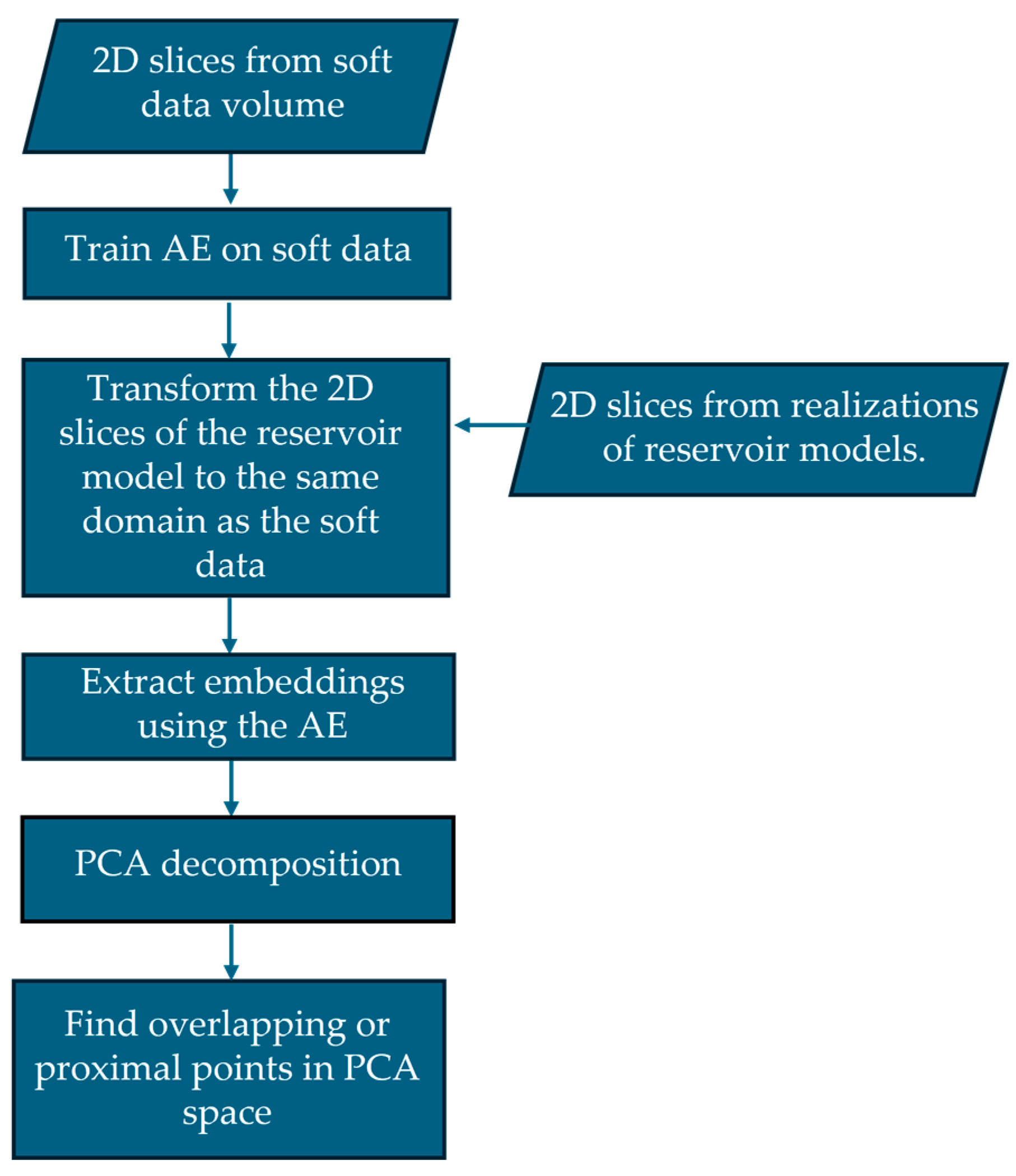
In this section, we describe our proposed workflow and its steps (in Figure 1).

• Extract 2D slices from the soft data 3D volume. If your data is already 2D, this step is not necessary;
• Train the AE on the soft data 2D slices, to calculate the mapping from soft data to latent space;
• Extract 2D slices from subsurface model realizations;
• Transform the 2D slices of the subsurface model to the same domain as the soft data, e.g., post-stack seismic, distribution transformations, etc.;
• Apply AE encoder to calculate latent space embeddings of both the soft data and the subsurface model;
• Perform PCA decomposition on the latent space embeddings of both the soft data and the subsurface model realizations.
• Find overlapping or proximal points in PCA space.

Depending on the source, soft data may already be available in a 2D format, for example, 2D seismic data, 2D gravimetric data, geological interpretations such as facies maps, remote sensing images, or outcrop photographs, which we refer to as 2D soft data slices. Multiple 2D soft data slices are required for effective AE training; therefore, image augmentation or additional analog images may be included.

If the soft data is provided in a 3D format, the volume is segmented into 2D soft data slices for effective AE training. It is advisable to orient these slices along the direction exhibiting the greatest heterogeneity, thereby enabling the AE to learn from the most informative variations. Additionally, the slicing should be dense and systematic to maximize the number of available training images.

Then the AE trains on 2D soft data slices to learn an efficient latent space representation. Training the AE on 2D slices instead of the full 3D soft data volume offers three key advantages. First, it dramatically reduces the computational complexity in computation and storage for training the AE model. Second, it increases the flexibility of the workflow, as soft data can already exist in a 2D format. Third, the AE requires a large number of training images to learn meaningful lower-dimensional embeddings. If the soft data consists of only a single 3D volume, the number of training samples is insufficient to properly train the AE. The 2D slices are a form of image augmentation, which improves the model’s ability to capture patterns and generalize effectively. Additionally, the AE is trained only on the soft data, and not the subsurface model realizations, to ensure that the generated latent space is tailored to the characteristics of the soft data. This allows the model to learn feature representations that accurately reflect the patterns and structures present in the soft data.

After training the AE, the 2D soft data slices used in training are encoded into a lower-dimensional latent representation. The size of these embeddings is described by an x-dimensional vector (i.e., a vector comprising x rows) based on the predefined latent space dimension, that is selected based on a balance between capturing sufficient geological features and avoiding redundant information and overfit. A smaller latent space may lose critical details, while a larger one may retain unnecessary noise. The size of the latent space is tuned with reconstruction error for the original soft data and inspection of the structure of the latent space.

The inspection of the latent structure within the latent space process involves evaluating the model’s ability to reconstruct the original data while preserving meaningful relationships among latent features, ensuring that similar soft data points remain close together. It is recommended to implement a feedback or iterative process to refine the selection of the latent space dimension. Additionally, this approach helps optimize computational efficiency by preventing the selection of an unnecessarily large latent space.

The 2D soft data slices are transformed to the same domain as the soft data (referred to as 2D transformed slices). This guarantees the subsurface model data to reside in the same domain as the soft data, facilitating effective encoding to the latent space of the autoencoder. This step enhances consistency between the soft data and the subsurface models. For example, the image distribution may be transformed to the soft data distribution, or a physics-based forward model may be applied, for example, in the case of seismic-based soft data as forward seismic transform is applied.

The trained AE is applied to the subsurface model 2D transformed slices. The embeddings extracted in this step summarize the most significant attributes of the 2D slices from the subsurface models’ realizations in the latent space of the soft data.

The dimensionality of the latent space is further reduced with Principal Component Analysis (PCA) to facilitate the comparison of the latent space representations of 2D soft data slices and the 2D transformed slices. PCA is a dimensionality reduction technique that applies an orthogonal transformation high-dimensional data into a smaller number of dimensions while preserving as much of the original variance as possible. The AE generated embeddings are reduced to two dimensions using PCA. This reduction allows for clear visualization and intuitive representation of the latent space. An additional advantage of PCA is that it allows new model realizations to be added dynamically. Once the autoencoder and PCA projection are trained, embeddings from any new model slices can be extracted and projected into the same PCA space without retraining or recomputing the entire dataset. This flexibility makes PCA particularly well suited for workflows that require iterative model evaluation. In contrast, other techniques such as Multidimensional Scaling (MDS) rely on pairwise similarity matrices that must be recalculated when new data are introduced, limiting their adaptability in this context.

The resulting two-dimensional projections of latent space embeddings are plotted to visualize the relative positions of the embeddings. For clarity, the projections of the 2D soft data slices are referred to as soft data points, while the projections of the 2D transformed slices corresponding to the subsurface models are referred to as model points. Soft data points are expected to lie close to or among the model points that better honor the soft data. This spatial proximity reflects greater similarity in their latent representations and helps assess how well a model aligns with the seismic data, as PCA organizes data points based on shared variance and underlying patterns.

The visual analysis of the latent space serves as an initial step in soft data checking, providing an intuitive way to assess the relationship between soft data slices and subsurface model slices. However, soft data volumes may consist of hundreds of slices, and subsurface models may include hundreds of realizations that are similarly divided into hundreds of slices, making it challenging to effectively visualize the proximity and alignment between the soft data and models in the 2D latent space, because the volume of data points can result in visual clutter, hindering the ability to draw clear conclusions.

To identify overlapping or proximal points in the PCA-transformed latent space using a quantitative method, the Euclidean distance between soft data points and model points for each subsurface model realization is calculated. This approach quantifies the similarity between the seismic and synthetic seismic embeddings by measuring their spatial proximity in the 2D PCA-transformed latent space.

The soft data points are denoted as $S_i=(x_{1,i},y_{1,i})$ for $i=1, \dots , N_s$, and the model points as $M_j=(x_{2,j},y_{2,j})$ for $j=1, \dots ,N_m$. The Euclidean distance is computed for each pair of points,

$$d_{ij}=\sqrt{{(x_{2,j}-x_{1,j})}^2+{(y_{2,j}-y_{1,j})}^2}$$

(6)

This distance calculation is applied across all soft data-model pairs. In addition, an indicator transform is employed to identify pairs of points that satisfy a predefined proximity criterion, defined by an indicator function $I_{ij}$ defined as

$$I_{ij}=\left\{\begin{array}{c}1, if d_{i,j}<threshold\\ 0, otherwise\hfill \end{array}\right.$$

(7)

where 1 indicates proximate and 0 not. For each subsurface model realization, the number of proximate or overlapping points—denoted as $n$—is determined by counting all soft data–model point pairs that satisfy the proximity condition $d_{ij}<threshold$ (i.e., where $I_{ij}=1$). This count serves as a quantitative measure of similarity; a higher $n$ indicates a greater alignment between the soft data and the subsurface models, since more soft data points are in close proximity to the model points in the PCA-transformed latent space. This analysis enables both visual and quantitative evaluation of the degree that subsurface models honor the soft data.

3. Results and Discussion

In this section, we introduce the datasets used to demonstrate our proposed workflow. These datasets are derived from rule-based models of deep marine environments and synthetic seismic data generated from these models to represent soft data. Then we describe the specific AE architecture employed and finally present the results and discussions of our proposed workflow.

3.1. Rule-Based Modeling and Synthetic Seismic Generation

Rule-based models are subsurface modeling techniques that simulate geological features by following predefined rules that mimic natural depositional processes. Unlike purely statistical models, rule-based approaches incorporate geological knowledge to generate realistic representations of geological formations. In deep marine environments, these models are particularly effective in capturing the hierarchical structure of depositional systems, where sediment bodies are arranged in layers or sequences that follow specific stacking patterns based on sedimentary processes [1,21].

GeoRulesLobePy [version 0.1.0] is a Python package designed to generate rule-based models of deep marine lobe systems [22]. These deepwater systems exhibit hierarchical structures, where the primary building block is the avulsion-bound sediment body. The largest scale in this hierarchy is called the lobe complex, which is made up of smaller, nested units. In GeoRulesLobePy, both lobes (as defined by [23]) or lobe elements (as described by [24]) are modeled as distinct avulsion-bound bodies that stack in a compensational manner to form these complexes. This architectural framework is based on the concept that avulsion-bound components aggregate to create progressively larger structures within the hierarchy [23,25].

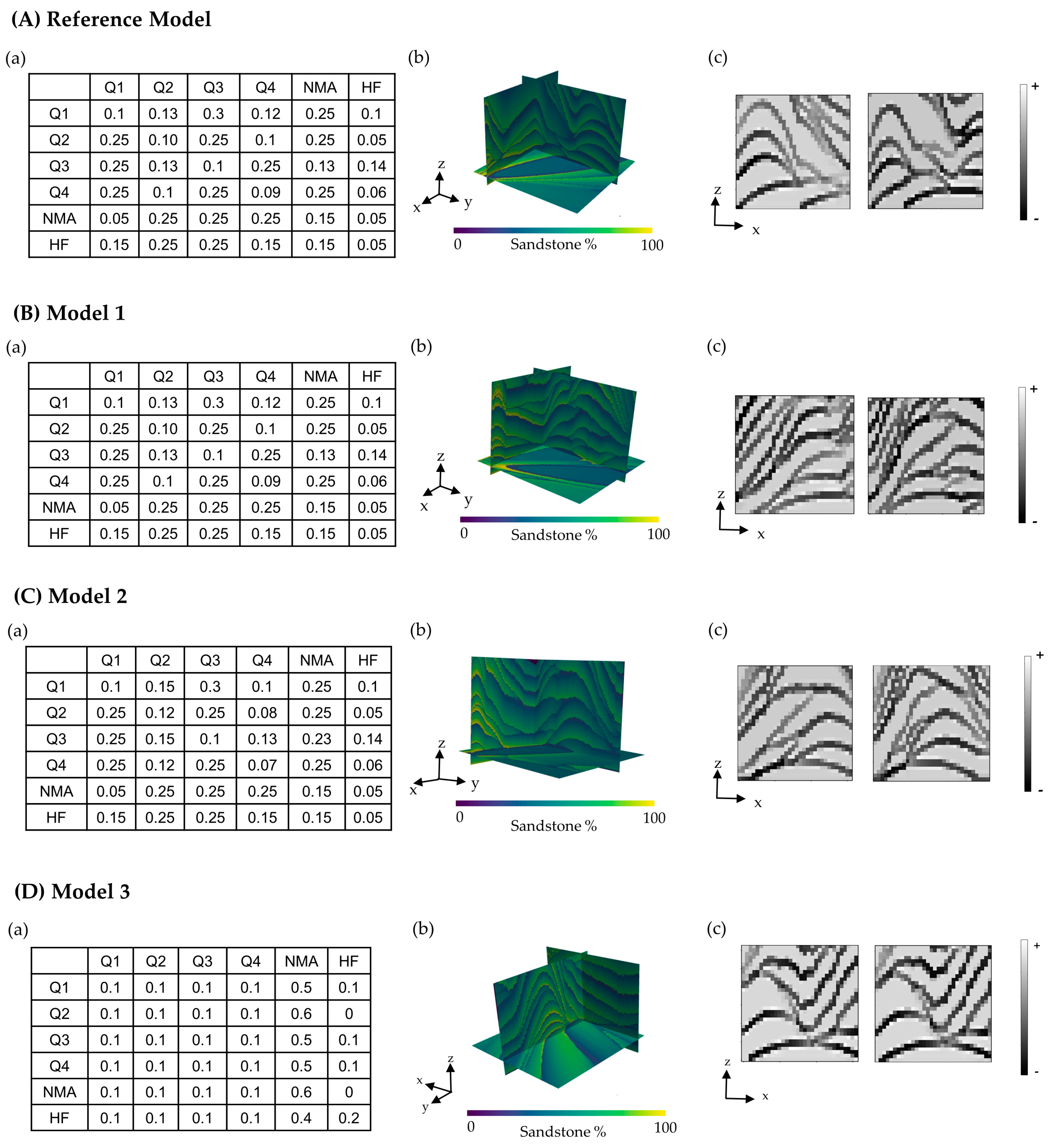
The rule-based model starts with an initial bathymetric surface. In each simulation step, a lobe element (sensu [24]) is added to the surface from the previous iteration. The placement of each lobe element is determined by a probability map and Markov chains transition probability. The placement of each lobe is guided by a probability map and Markov chain transition probabilities. The probability map is inversely related to the topography, filling depressions, following the principle of compensational stacking [24,25,26,27]. GeoRulesLobePy employs Markov chains where states represent different stacking patterns and transition probabilities represent the likelihood of moving between them. The Markov transition probabilities are the probabilities assigned to transitioning from one state to another or remaining in the same state. The six states are: Q1 (regression), Q3 (transgression), Q2 and Q4 (lateral offset), NMA (major avulsion), and HF (hiatus marked by fine-grained deposition; see [22] for more information). After each lobe is added, the topography is updated, altering the probability map for subsequent lobe placement. This sequential process continues until the user-defined number of lobe elements is achieved.

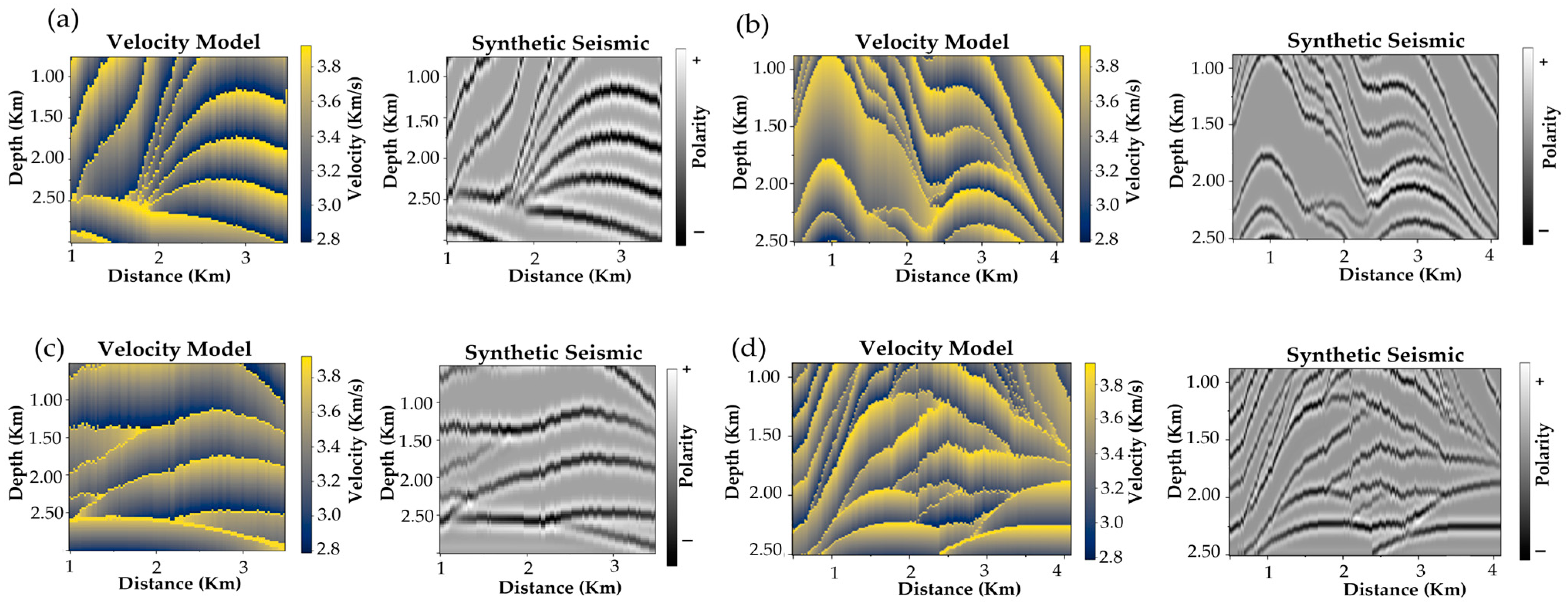
For this application, GeoRulesLobePy generates 3D velocity models of the resultant rule-based models, which are sliced along the x–z axis to produce 2D velocity models. We generate synthetic data from the output velocity models using the PostastackLinearModelling operator, from the PyLops Python package, which models post-stack seismic data [28] (Figure 2). A Ricker wavelet of is employed to simulate the seismic source wavelet, 10 Hz–25 Hz were used in the modeling as this range of frequencies provide enough resolution to identify the lobe elements in the synthetic seismic. Gaussian noise was added to the synthetic seismic to mimic real-world seismic data conditions.

3.2. AE Architecture

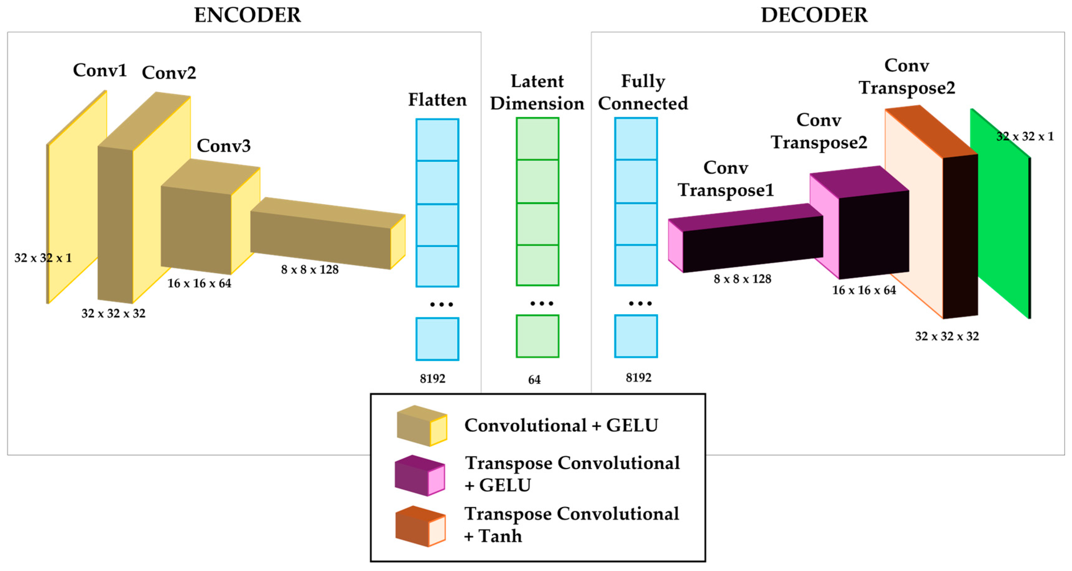
The AE (Figure 3) input is a 32 × 32 × 1 array, representing a grayscale image with pixel values normalized to the range [−1,1]. The encoder compresses this input through three convolutional layers, each followed by a Gaussian Error Linear Unit (GELU) activation function, progressively downsizing the array to 8 × 8 × 128. This array is then flattened into a one-dimensional vector of size 8192 × 1, from which the latent representation is extracted. The latent dimension, which is set to 64 × 1 in this study. The decoder reconstructs the input by first mapping the latent representation back to 8192 × 1 through a fully connected layer, followed by three transpose convolutional layers. The first two transpose convolutional layers use GELU activation functions to progressively up-sample the data, and the final transpose convolutional layer employs a hyperbolic tangent (Tanh) activation function to ensure that the reconstructed output matches the input’s range of [−1, 1].

The model was implemented in PyTorch Lightning [version 1.8.0] and trained using the Adam optimizer with a learning rate of 1 × 10⁻³, a batch size of 64, and a maximum of 500 epochs. A ReduceLROnPlateau scheduler was used to reduce the learning rate by a factor 0.2 after 20 epochs without improvement, with a minimum learning rate of 5 × 10⁻⁵. The mean square error (MSE) was used as the reconstruction loss, summed over all pixels and averaged over the batch. Batch normalization was intentionally omitted to avoid introducing dependencies across images, ensuring that each slice’s encoding remained independent. Model selection was based on validation loss, with the best-performing model retained. Training was conducted on a single GPU. Visual reconstructions were logged during training using TensorBoard to monitor convergence and reconstruction quality. The full implementation and training scripts are available in the Supplementary Material Section.

3.3. Workflow Demonstration

To demonstrate the proposed workflow, a single reference, truth rule-based model is used (see Figure 4), with its associated synthetic 2D seismic slices serving as the soft data, while the reservoir model scenarios include models 1, 2 and 3. Model 1 (see Figure 4) shares the same Markov chain conditional probabilities as the reference rule-based model. In contrast, model 2 (see Figure 4) has some different conditional probabilities from model 1’s Markov chain, while Model 3 (see Figure 4) features a completely different Markov chain compared to the other models. The AE is trained using the 200 2D soft data slices to generate a latent space informed by the soft data. The trained AE is then applied to each of the 200 slices from Model 1, Model 2, and Model 3 to extract their corresponding embeddings.

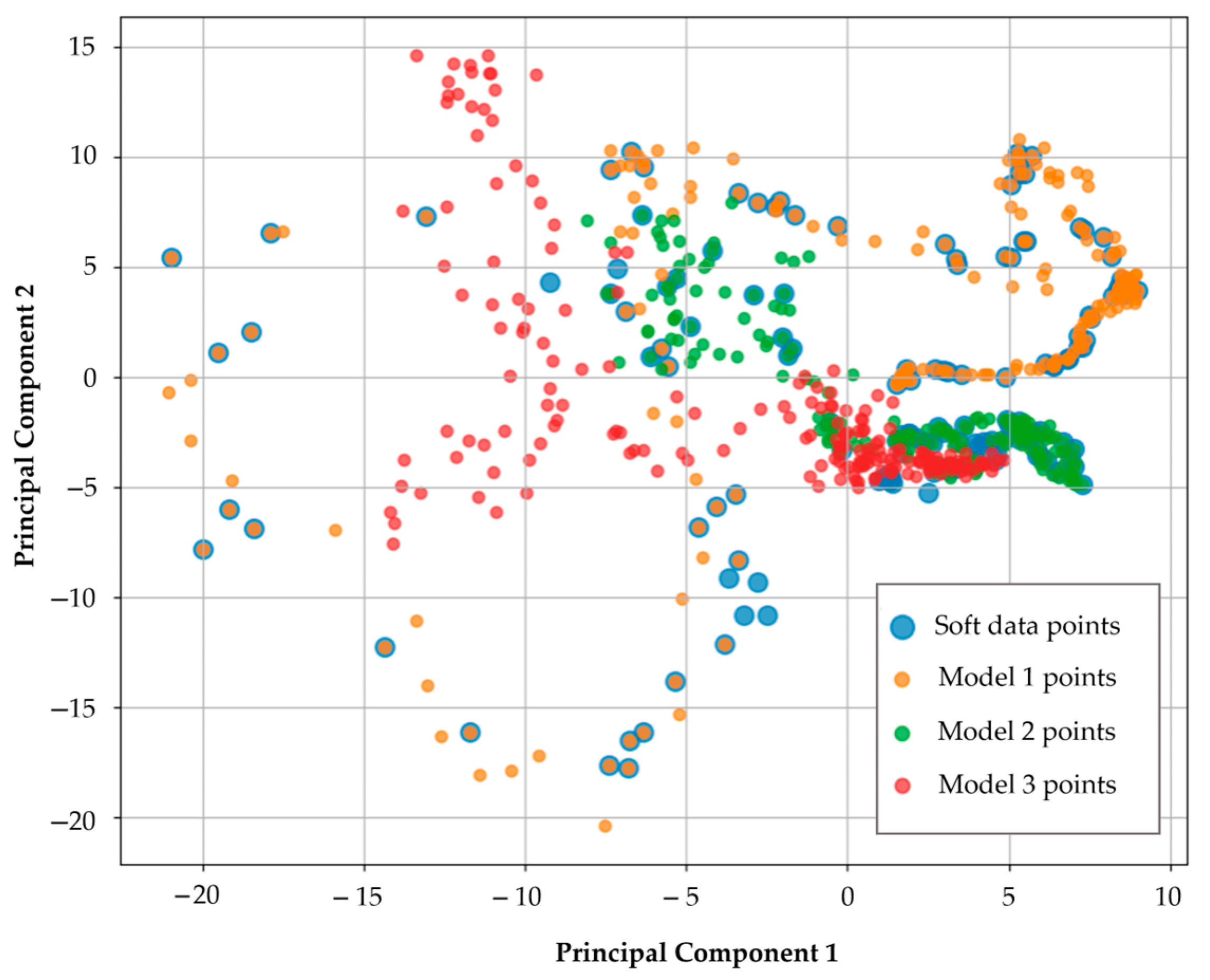
To analyze these embeddings, PCA is performed to reduce the dimensionality of the embeddings to a 2D space, and the resulting soft data points and model points are plotted (see Figure 5). Model 1 points, which correspond to the subsurface model most similar to the soft data in terms of Markov chain parameters, are observed to cluster near the soft data points in the PCA space. Model 2 points appear farther away, while Model 3 points, which are based on a markedly different Markov chain, show the greatest separation. This spatial arrangement reflects the underlying differences in input parameters, supporting the idea that similarity in input space is preserved in the learned latent space.

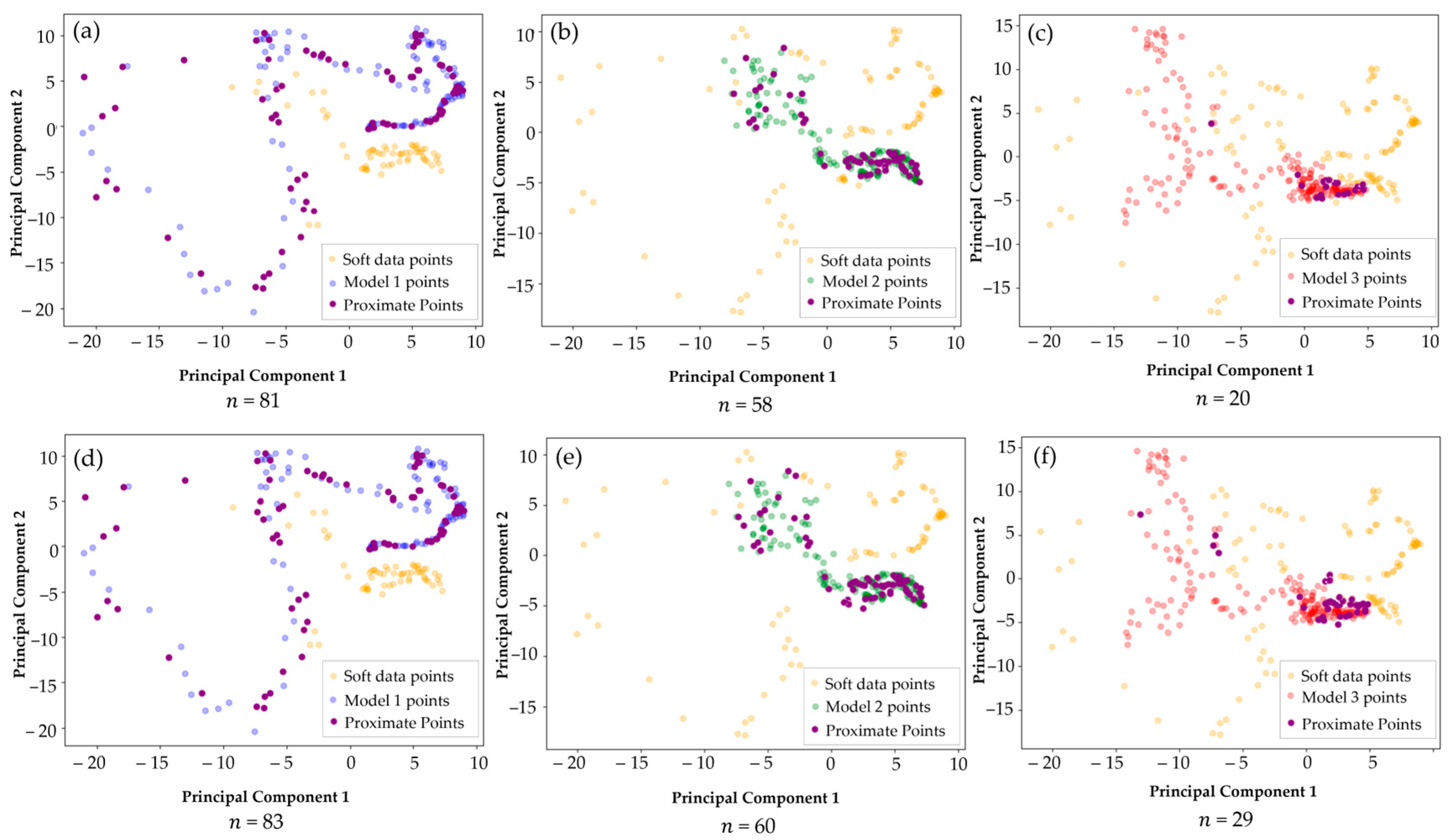
To quantify this relationship, we computed the Euclidean distance between the seismic points and the model points. In Figure 6, parts a–c, the threshold distance is set to 0.5, the number of proximate points ($n$) is highest for subsurface model 1 and decreases for subsurface model 3. A similar trend is observed in Figure 6, parts d–f, for an increase in threshold distance to 0.7. Our proposed method scores the highest soft data conditioning for subsurface model 1, which is expected since this model shares similar Markov chains and input parameters with the soft data. The quantification of proximity and overlap of embeddings in the latent space highlights the strength of this approach in quantitatively determining how well different subsurface models honor the provided soft data.

The Euclidean distance between the seismic points and the subsurface model points for each subsurface model are calculated. In Figure 6, parts a–c, the threshold distance is set to 0.5, the number of proximate points ($n$) is highest for subsurface model 1 and decreases for subsurface model 3. A similar trend is observed in Figure 6, parts d–f, for an increase in threshold distance to 0.7.

Our proposed method scores the highest soft data conditioning for subsurface model 1, which is expected since this model shares similar Markov chains and input parameters with the soft data. The quantification of proximity and overlap of embeddings in the latent space highlights the strength of this approach in quantitatively determining how well different subsurface models honor the provided soft data. This result highlights a key strength of the approach: by compressing soft data and model slices into a latent space using an AE trained on the soft data, we extract representations relevant to geologic behavior. These latent embeddings allow comparisons based on learned feature similarity, rather than relying solely on pixel-based or global similarity metrics.

The quantification of proximity and overlap in the latent space (Figure 6) confirms that models with more geologically consistent input parameters tend to be closer to the soft data in the 2D latent space. This supports the idea that our method allows for a more geologically meaningful similarity assessment.

4. Conclusions

We introduced a novel workflow for soft data checking, by quantifying the similarity between soft data and subsurface model realizations within a low-dimensional latent space. By training an autoencoder on soft data, the workflow generates embeddings that capture the essential structural and visual characteristics of the soft data. These embeddings form the basis for quantitatively comparing subsurface models to soft data using techniques such as PCA for dimensionality reduction and Euclidean distance for proximity analysis.

The results demonstrate the effectiveness of this workflow in assessing the ability of subsurface models to honor soft data, with models better conditioned to the seismic data scoring higher via quantification of proximity in the latent space. This approach not only fulfills the need for quantitative soft data checking but also provides a robust framework for evaluating the consistency between soft data and subsurface models, for example, geophysical data and subsurface models for hydrocarbons, gravity surveys and ore bodies, and land use maps and groundwater aquifers.

The proposed workflow is limited by its reliance on large datasets, for example, more than 100 training images, requiring the slicing of 3D data into 2D images or the application of image augmented, for example, generating additional, consistent images through simulations or generative AI, to train the autoencoder effectively. Future work could include methods to extend the proposed workflow to situations with limited data points, for example, a single 2D seismic slice or a few geologic profiles.

References

1. Pyrcz, M.J.; Deutsch, C.V. Geostatistical Reservoir Modeling, 2nd ed.; Oxford University Press: New York, NY, USA, 2014. [Google Scholar]
2. Rossi, M.E.; Deutsch, C.V. Mineral Resource Estimation, 1st ed.; Springer: Dordrecht, The Netherlands, 2014. [Google Scholar]
3. Michael, H.A.; Li, H.; Boucher, A.; Sun, T.; Caers, J.; Gorelick, S.M. Combining geologic-process models and geostatistics for conditional simulation of 3-D subsurface heterogeneity. Water Resour. Res. 2010, 46, W05527. [Google Scholar] [CrossRef]
4. Schnaar, G.; Digiulio, D.C. Computational Modeling of the Geologic Sequestration of Carbon Dioxide. Vadose Zone J. 2009, 8, 389–403. [Google Scholar] [CrossRef]
5. Leuangthong, O.; Mclennan, J.A.; Deutsch, C.V. Minimum Acceptance Criteria for Geostatistical Realizations. Nat. Resour. Res. 2004, 13, 131–141. [Google Scholar] [CrossRef]
6. Boisvert, J.B.; Pyrcz, M.J.; Deutsch, C.V. Multiple-point statistics for training image selection. Nat. Resour. Res. 2007, 16, 313–321. [Google Scholar] [CrossRef]
7. Deutsch, C.V.; Journel, A.G. GSLIB: Geostatistical Software Library and User’s Guide, 2nd ed.; Oxford University Press: New York, NY, USA, 1997. [Google Scholar]
8. Strebelle, S.; Levy, M. Using multiple-point statistics to build geologically realistic reservoir models: The MPS/FDM workflow. Geol. Soc. Lond. Spec. Publ. 2008, 309, 67–74. [Google Scholar] [CrossRef]
9. Wang, Z.; Bovik, A.C.; Sheikh, H.R.; Simoncelli, E.P. Image Quality Assessment: From Error Visibility to Structural Similarity. IEEE Trans. Image Process. 2004, 13, 1–14. [Google Scholar] [CrossRef]
10. Wang, Z.; Simoncelli, E.P. Translation Insensitive Image Similarity in Complex Wavelet Domain. In Proceedings of the IEEE International Conference on Acoustic, Speech, and Signal Processing, Philadelphia, PA, USA, 23 March 2005. [Google Scholar] [CrossRef]
11. Simard, P.Y.; LeCun, Y.A.; Denker, J.S.; Victorri, B. Transformation Invariance in Pattern Recognition—Tangent Distance and Tangent Propagation. In Neural Networks: Tricks of the Trade; Springer: Berlin/Heidelberg, Germany, 2012; pp. 235–269. [Google Scholar] [CrossRef]
12. Wang, Z.; Bovik, A.C. A Universal Image Quality Index. IEEE Signal Process. Lett. 2002, 9, 81–84. [Google Scholar] [CrossRef]
13. Zhang, L.; Zhang, L.; Mou, X.; Zhang, D. FSIM: A feature similarity index for image quality assessment. IEEE Trans. Image Process. 2011, 20, 2378–2386. [Google Scholar] [CrossRef] [PubMed]
14. Xu, S.; Liu, X.; Jiang, S. A Fast Feature Similarity Index for Image Quality Assessment. Int. J. Signal Process. Image Process. Pattern Recognit. 2015, 8, 179–194. [Google Scholar] [CrossRef]
15. Al-Marzouqi, H.; AlRegib, G. Similarity index for seismic data sets using adaptive curvelets. In SEG Technical Program Expanded Abstracts; Society of Exploration Geophysicists: Tulsa, OK, USA, 2014; Volume 33, pp. 1470–1474. [Google Scholar] [CrossRef]
16. Yang, N.; Duan, Y. Human vision system-based structural similarity model for evaluating seismic image quality. Geophysics 2018, 83, F49–F54. [Google Scholar] [CrossRef]
17. Baldi, P. Autoencoders, Unsupervised Learning, and Deep Architectures. In Proceedings of the 2011 International Conference on Unsupervised and Transfer Learning Workshop, Washington, DC, USA, 2 July 2012; Volume 27, pp. 37–50. [Google Scholar]
18. Vincent, P.; Larochelle, H.; Bengio, Y.; Manzagol, P.-A. Extracting and Composing Robust Features with Denoising Autoencoders. In Proceedings of the 25th International Conference on Machine Learning, Helsinki, Finland, 5–9 July 2008; pp. 1096–1103. [Google Scholar]
19. Olshausen, B.A.; Field, D.J. Emergence of simple-cell receptive field properties by learning a sparse code for natural Images. Nature 1996, 381, 607–609. [Google Scholar] [CrossRef] [PubMed]
20. Fernández, S.T. Designing Variational Autoencoders for Image Retrival; DiVA Portal: Uppsala, Sweden, 2018. [Google Scholar]
21. Jo, H.; Pyrcz, M.J. Robust Rule-Based Aggradational Lobe Reservoir Models. Nat. Resour. Res. 2020, 29, 1193–1213. [Google Scholar] [CrossRef]
22. Chacon-Buitrago, N.; Willhelm, D. GeoRulesLobePy, Version 0.1.1. 2025. Available online: https://github.com/chaconnb/GeoRulesLobePy (accessed on 20 July 2025).
23. Prélat, A.; Covault, J.A.; Hodgson, D.M.; Fildani, A.; Flint, S.S. Intrinsic controls on the range of volumes, morphologies, and dimensions of submarine lobes. Sediment. Geol. 2010, 232, 66–76. [Google Scholar] [CrossRef]
24. Straub, K.M.; Pyles, D.R. Quantifying the hierarchical organization of compensation in submarine fans using surface statistics. J. Sediment. Res. 2012, 82, 889–898. [Google Scholar] [CrossRef]
25. Sweet, M.L.; Gaillot, G.T.; Jouet, G.; Rittenour, T.M.; Toucanne, S.; Marsset, T.; Blum, M.D. Sediment routing from shelf to basin floor in the Quaternary Golo System of Eastern Corsica, France, western Mediterranean Sea. Bull. Geol. Soc. Am. 2020, 132, 1217–1234. [Google Scholar] [CrossRef]
26. Mutti, E.; Sonnino, M. Compensation cycles: A diagnostic feature of turbidite sandstone lobes. In Proceedings of the International Association of Sedimentologists―European Regional Meeting, Bologna, Italy; 1981; Volume 2, pp. 120–123. [Google Scholar]
27. Straub, K.M.; Paola, C.; Mohrig, D.; Wolinsky, M.A.; George, T. Compensational stacking of channelized sedimentary deposits. J. Sediment. Res. 2009, 79, 673–688. [Google Scholar] [CrossRef]
28. Ravasi, M.; Vasconcelos, I. PyLops—A linear-operator Python library for scalable algebra and optimization. SoftwareX 2020, 11, 100361. [Google Scholar] [CrossRef]
Figure 1. Flowchart of the proposed workflow.
Geosciences 15 00288 g001
Figure 2. Panels (ad) show slices of velocity models derived from reservoir models alongside their corresponding synthetic seismic responses.
Geosciences 15 00288 g002
Figure 3. Autoencoder architecture used to demonstrate the proposed workflow.
Geosciences 15 00288 g003
Figure 4. The GeoRulesLobePy rule-based reference truth model, and 3 model cases. In the Markov chain transition probability matrix, each cell represents the probability of transitioning from the state indicated by the column to the state indicated by the row (a), sections of the sandstone percentage model (b) and 2D seismic slices for each model (c).
Geosciences 15 00288 g004
Figure 5. PCA of AE embeddings with soft data points and Subsurface model points for Models 1, 2, 3, shown.
Geosciences 15 00288 g005
Figure 6. Overlapping or proximal points between the soft data and each Subsurface model. Graphs (ac) present the results for a threshold distance of 0.5, while graphs (df) display the results for a threshold distance of 0.7. The value n represents the percentage of overlapping or proximal points, which are highlighted in purple in the graphs.
Geosciences 15 00288 g006
Disclaimer/Publisher’s Note: The statements, opinions and data contained in all publications are solely those of the individual author(s) and contributor(s) and not of MDPI and/or the editor(s). MDPI and/or the editor(s) disclaim responsibility for any injury to people or property resulting from any ideas, methods, instructions or products referred to in the content.