


Investigating a Large-Scale Creeping Landmass Using Remote Sensing and Geophysical Techniques—The Case of Stropones, Evia, Greece

 , , , , and
Abstract
1. Introduction
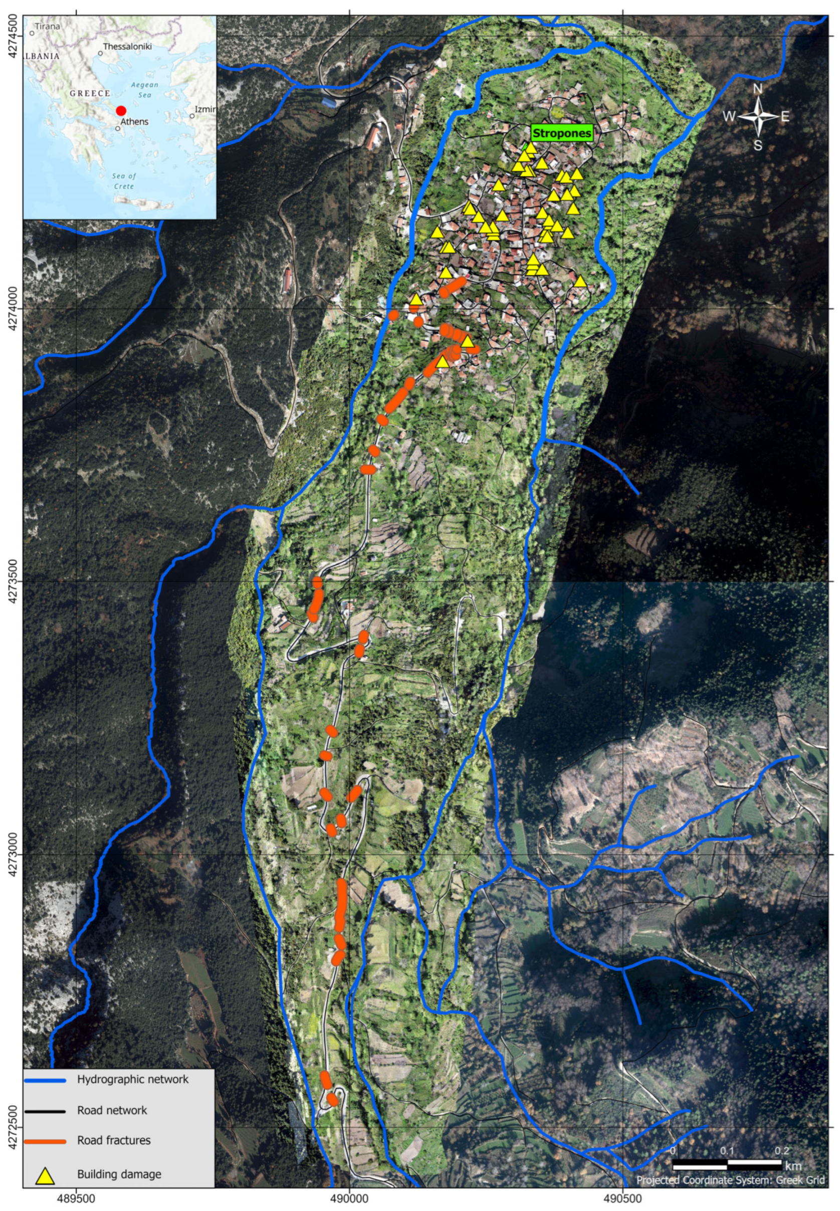
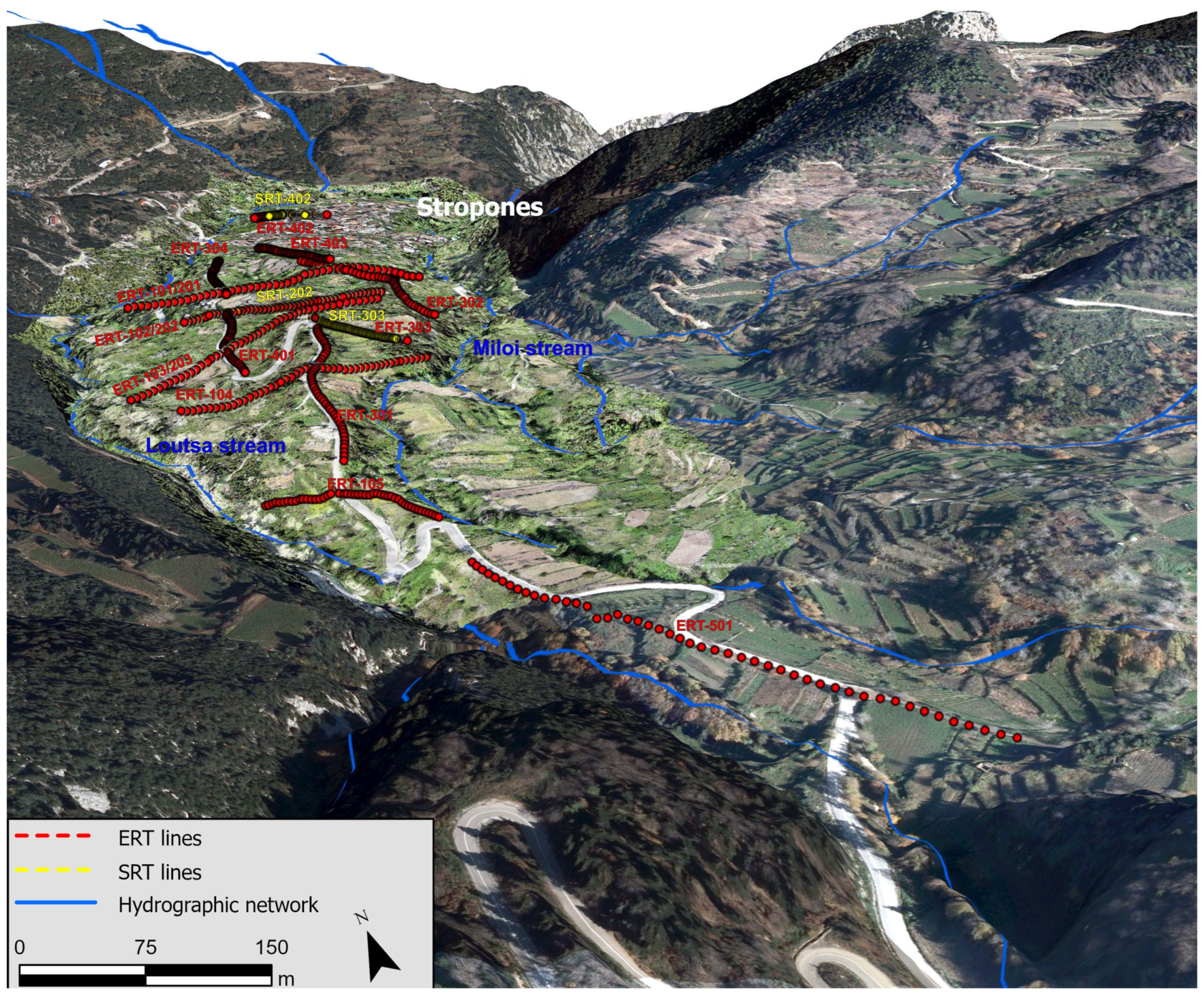
2. Study Area
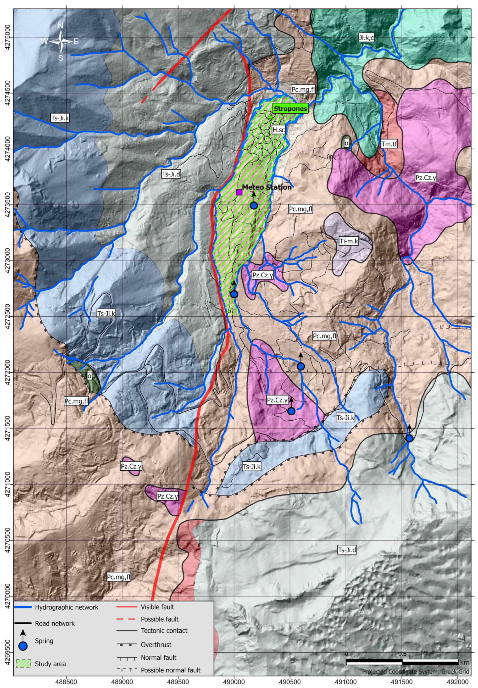
2.1. Geology
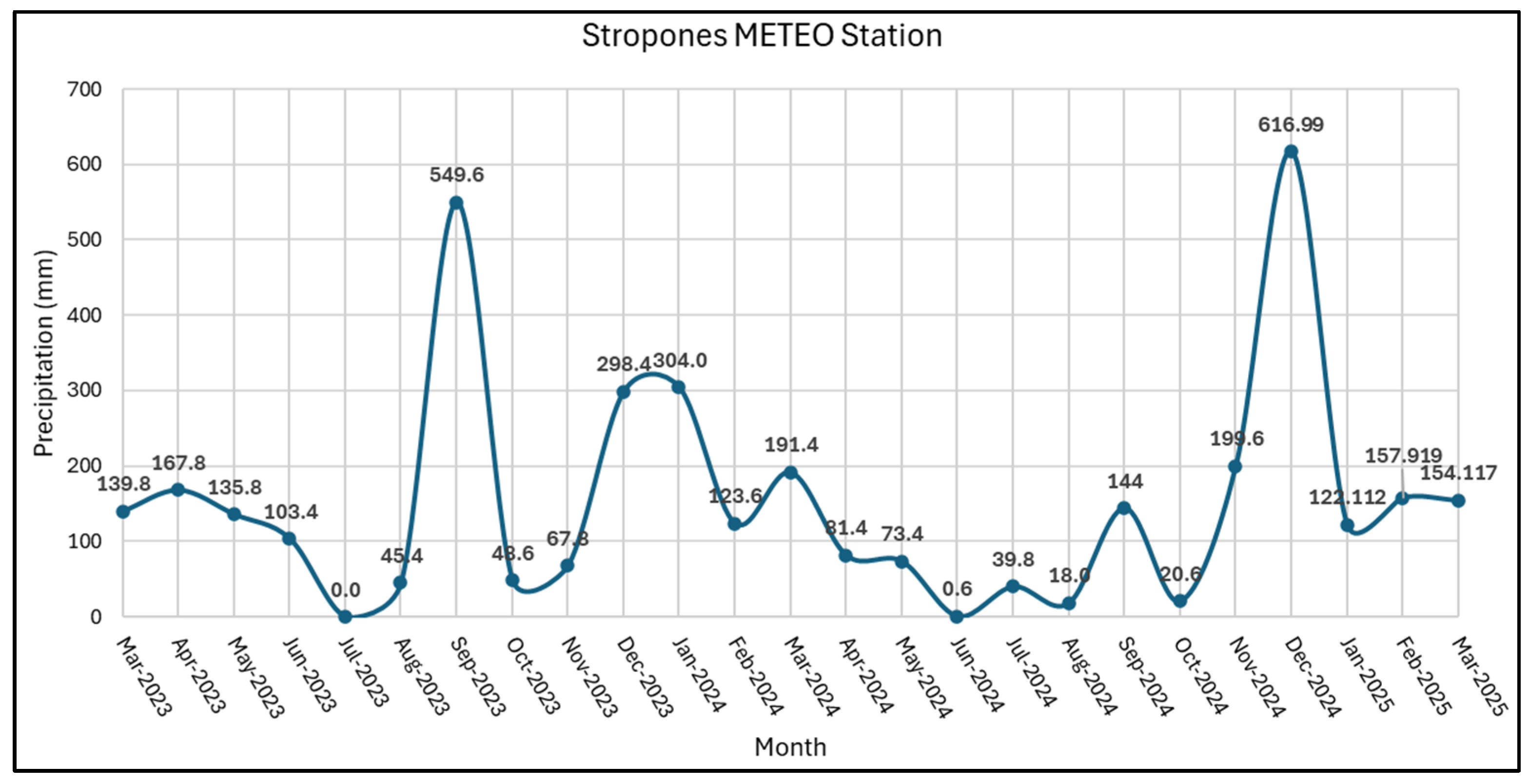
2.2. Climate Characteristics
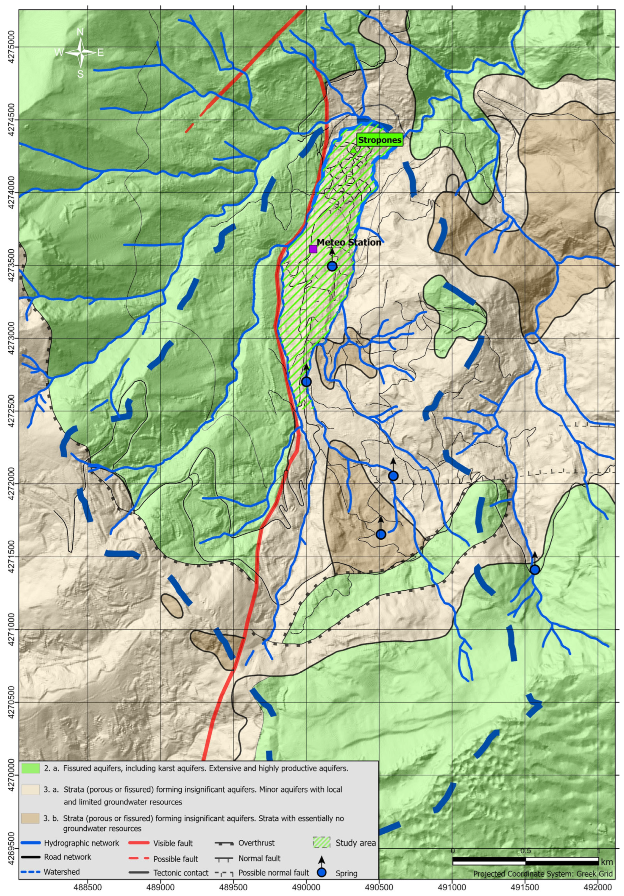
2.3. Hydrogeology
- 1.
- Cohesive (mainly carbonate) formations with secondary permeability.
- 2.
- Granular or fissured formations with limited or no groundwater concentration.
- Locally significant groundwater, primarily in zones of fracturing and weathering of cohesive formations. This subcategory includes the volcanic-sedimentary series of the Middle Triassic (Tm.tf), and the main mass of the tectonic mélange (Pc.mg,fl). In this area, due to the intense fragmentation, the development of secondary porosity and atmospheric precipitation, the formations of this subcategory are also aquiferous.
- Strata with essentially no groundwater resources. This subcategory includes Paleozoic granites (Pz.Cs.γ).
3. Methodology
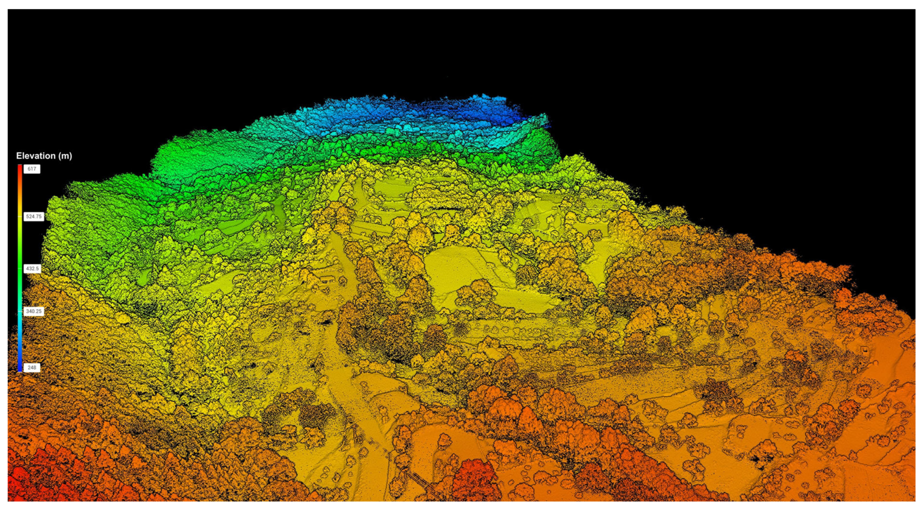
3.1. Remote Sensing Techniques
3.2. Geophysical Investigation
3.2.1. Electrical Resistivity Tomography
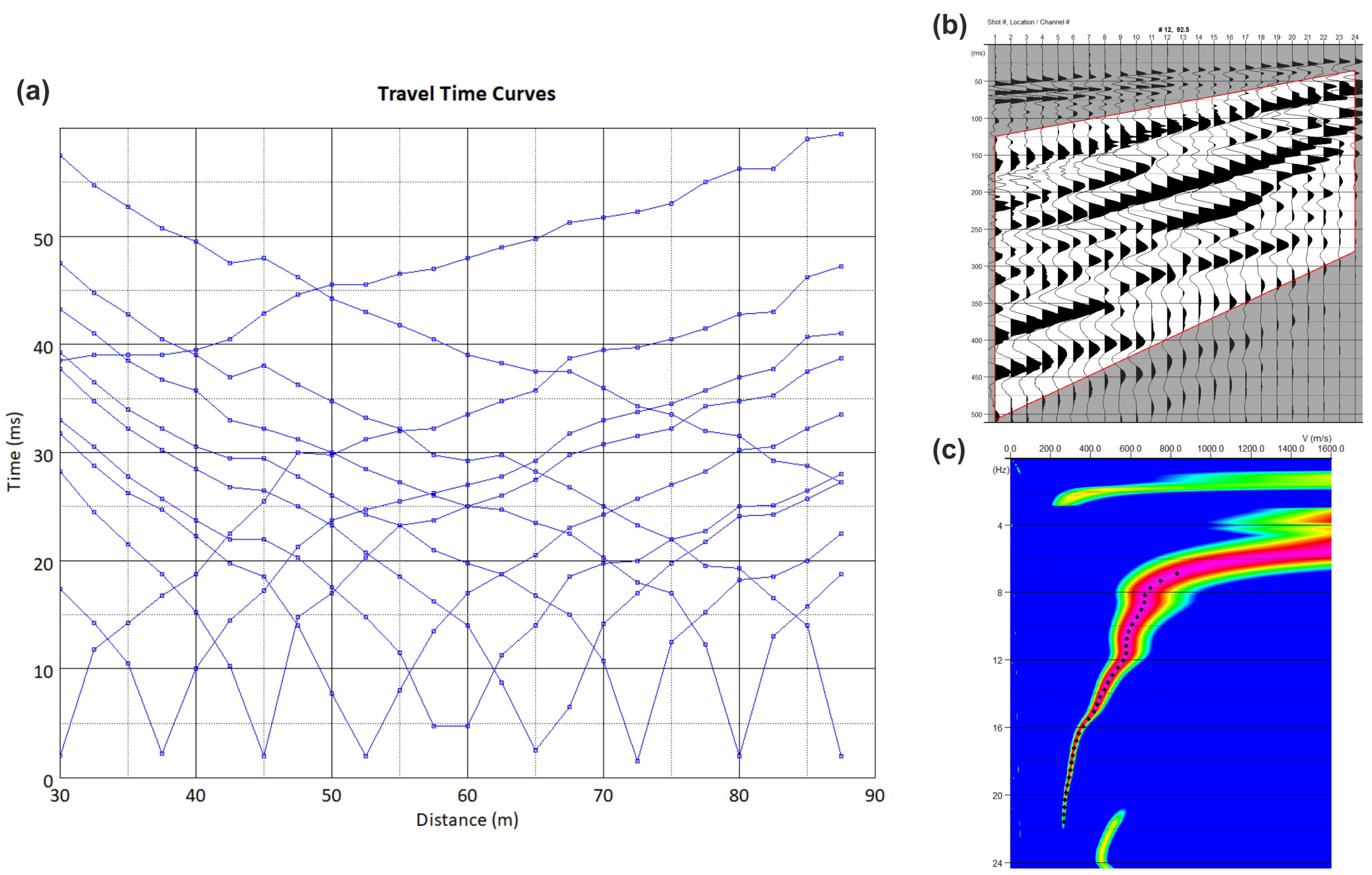
3.2.2. SRT and MASW Techniques
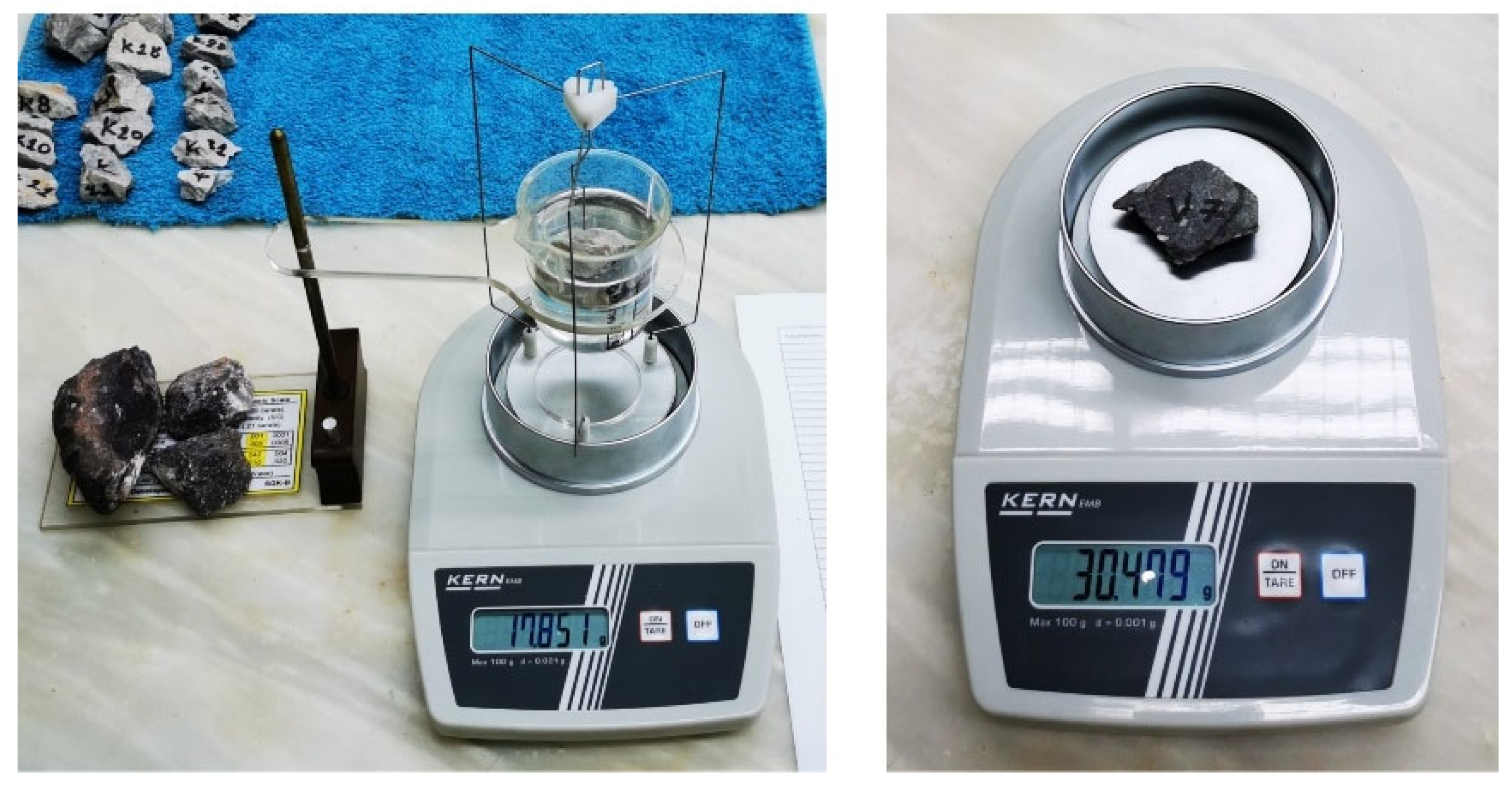
3.3. Laboratory Density Determination
4. Results and Interpretation
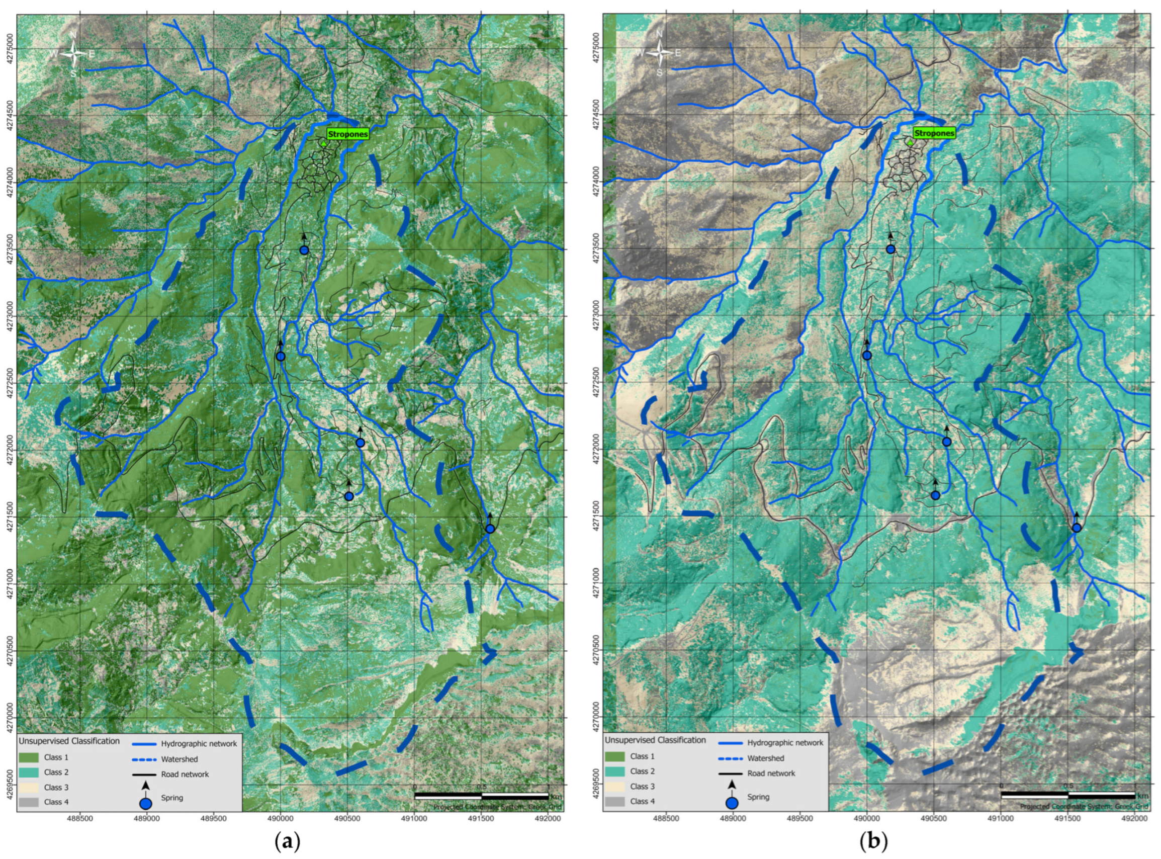
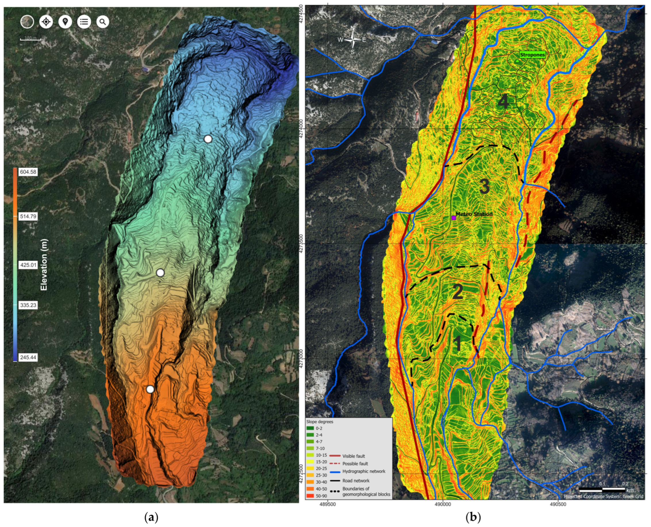
4.1. Remote Sensing
4.2. Combined Geophysical Investigation
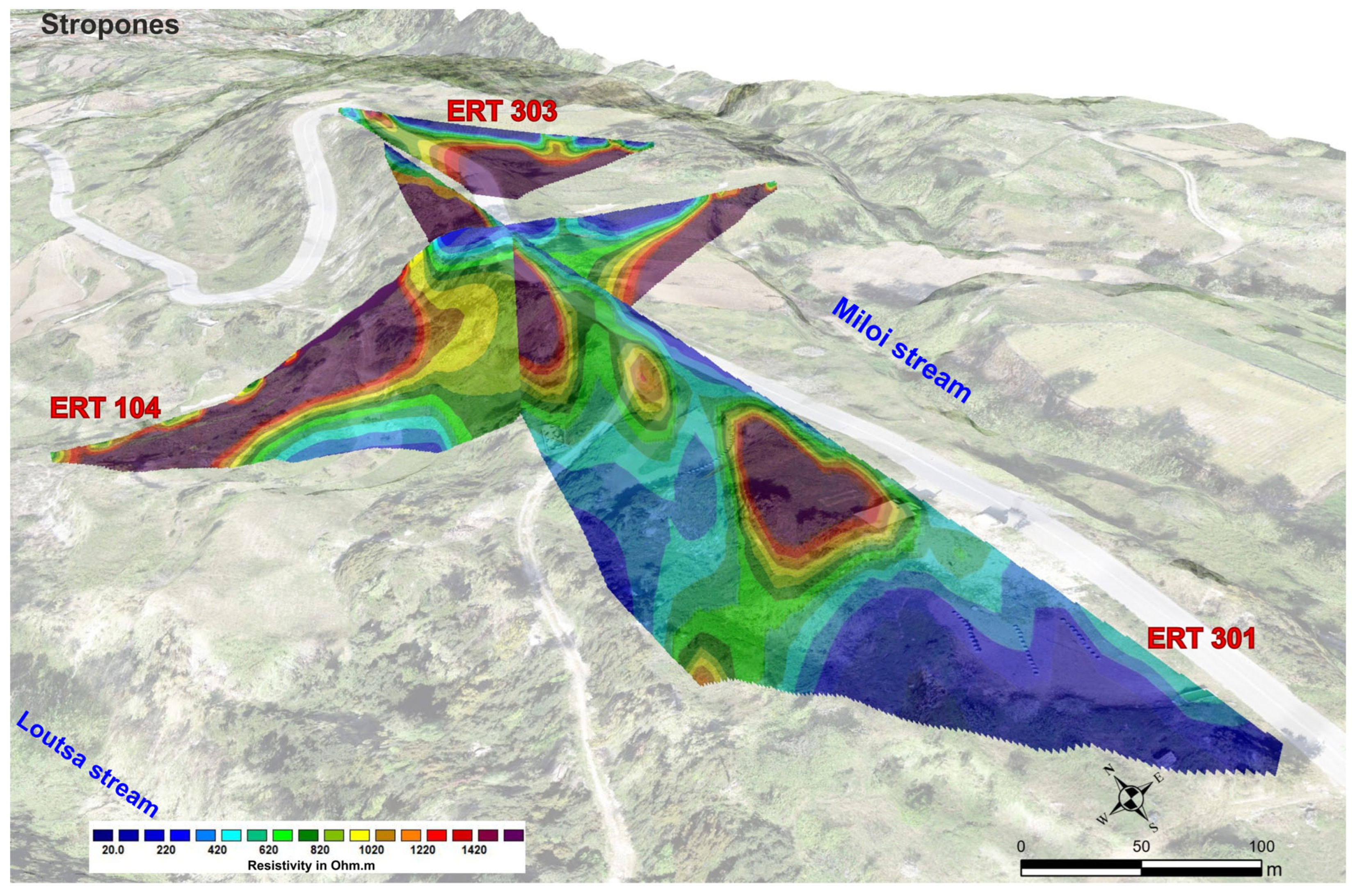
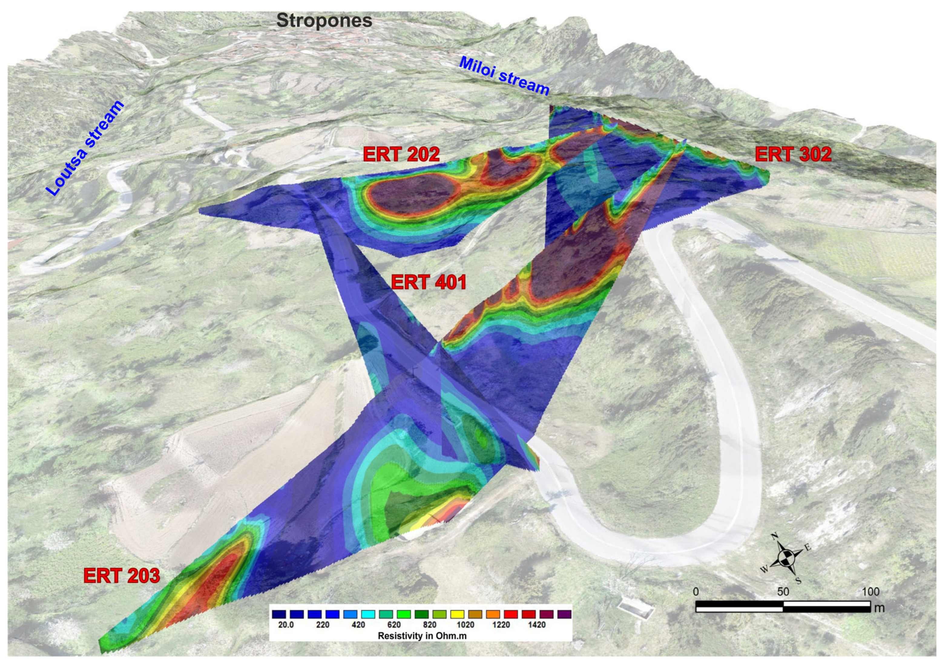
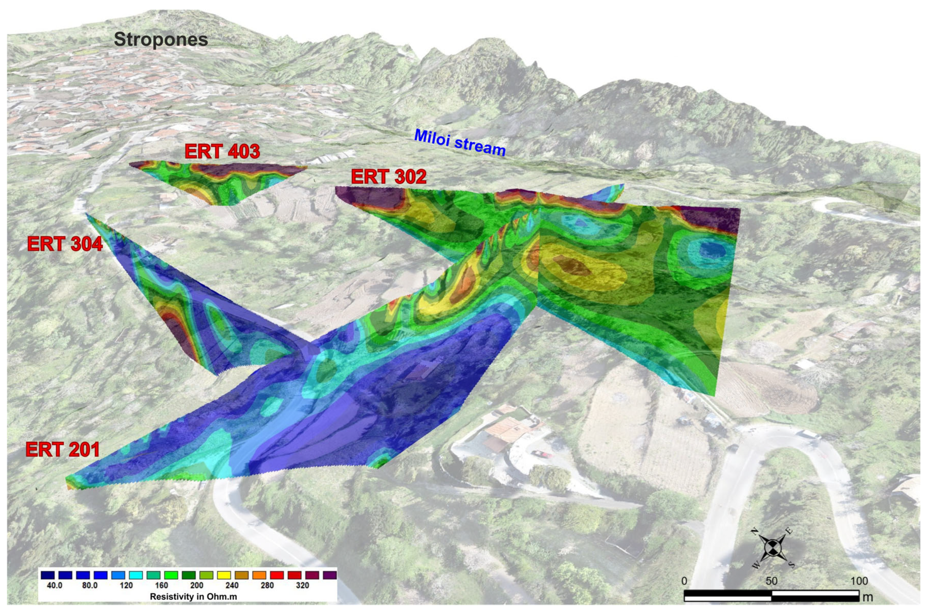
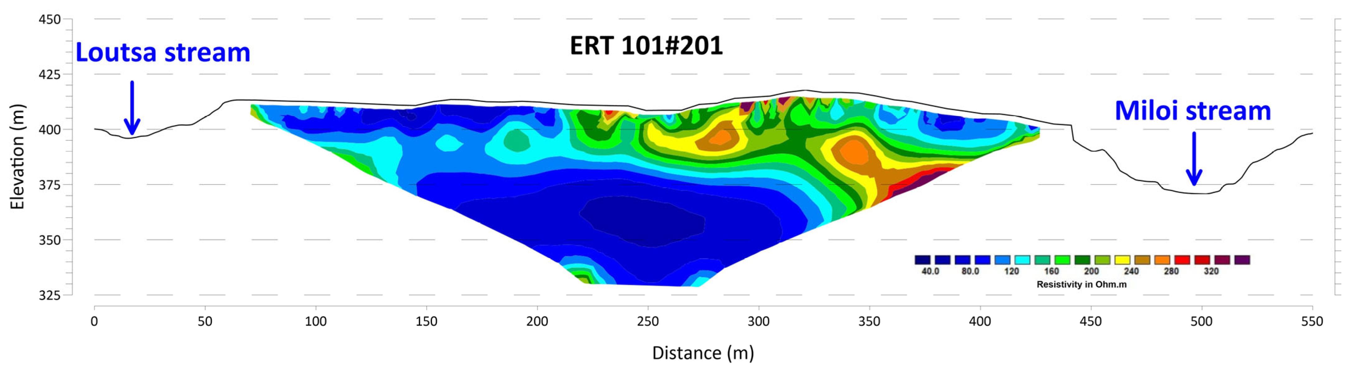
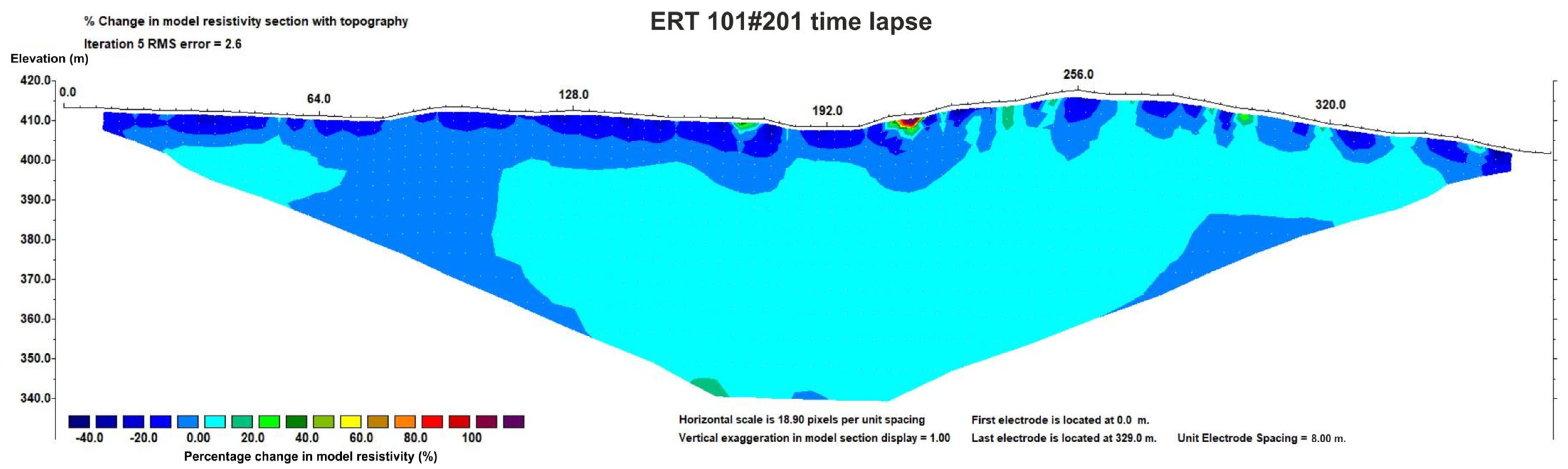
4.2.1. ERT Results
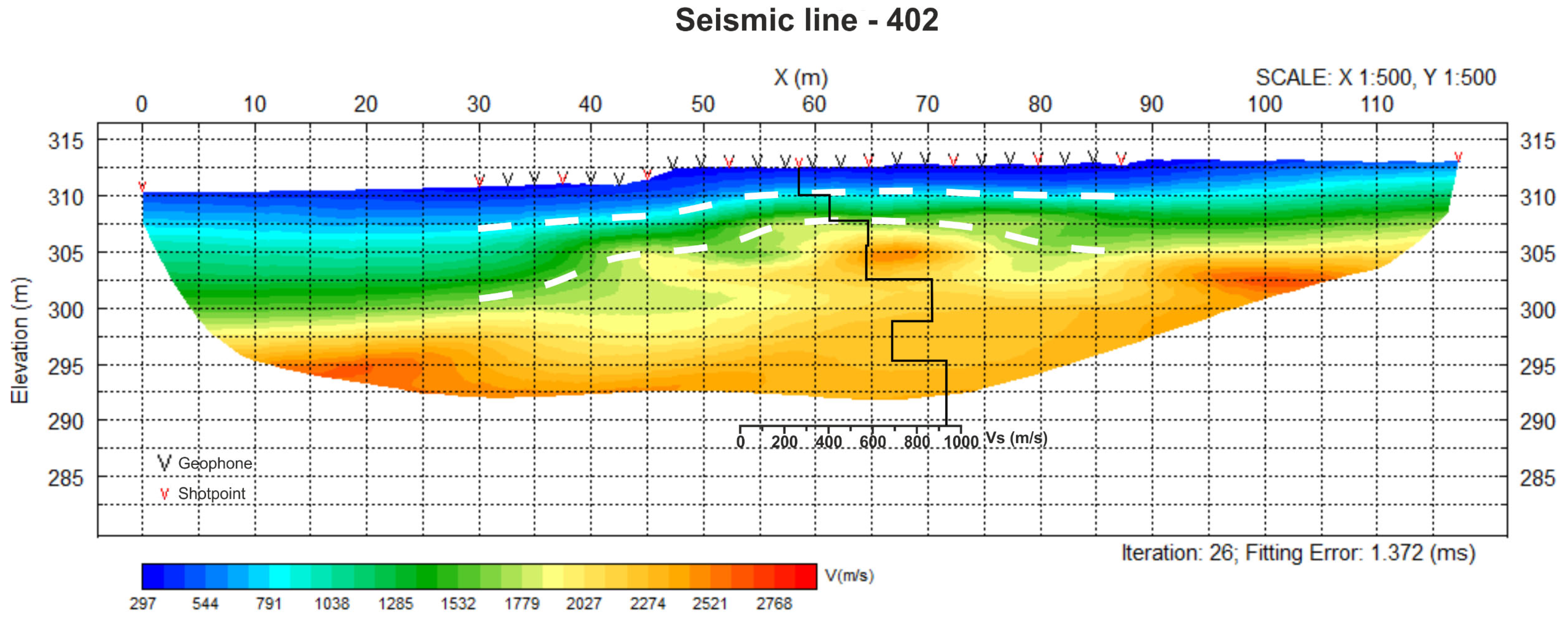
4.2.2. SRT and MASW Results
5. Discussion
6. Conclusions
Author Contributions
Funding
Data Availability Statement
Acknowledgments
Conflicts of Interest
References
- Froude, M.J.; Petley, D.N. Global fatal landslide occurrence from 2004 to 2016. Nat. Hazards Earth Syst. Sci. 2018, 18, 2161–2181. [Google Scholar] [CrossRef]
- Himi, M.; Anton, M.; Sendrós, A.; Abancó, C.; Ercoli, M.; Lovera, R.; Deidda, G.P.; Urruela, A.; Rivero, L.; Casas, A. Application of resistivity and seismic refraction tomography for landslide stability assessment in Vallcebre, Spanish Pyrenees. Remote Sens. 2022, 14, 6333. [Google Scholar] [CrossRef]
- Palmer, J. Creeping earth could hold secret to deadly landslides. Nature 2017, 548, 384–386. [Google Scholar] [CrossRef] [PubMed]
- Mansour, M.F.; Morgenstern, N.R.; Martin, C.D. Expected damage from displacement of slow-moving slides. Landslides 2011, 8, 117–131. [Google Scholar] [CrossRef]
- Nappo, N.; Peduto, D.; Mavrouli, O.; van Westen, C.J.; Gullà, G. Slow-moving landslides interacting with the road network: Analysis of damage using ancillary data, in situ surveys and multi-source monitoring data. Eng. Geol. 2019, 260, 105244. [Google Scholar] [CrossRef]
- Lacroix, P.; Dehecq, A.; Taipe, E. Irrigation-triggered landslides in a Peruvian desert caused by modern intensive farming. Nat. Geosci. 2020, 13, 56–60. [Google Scholar] [CrossRef]
- Schulz, W.H.; Smith, J.B.; Wang, G.; Jiang, Y.; Roering, J.J. Clayey landslide initiation and acceleration strongly modulated by soil swelling. Geophys. Res. Lett. 2018, 45, 1888–1896. [Google Scholar] [CrossRef]
- Mainsant, G.; Larose, E.; Brönnimann, C.; Jongmans, D.; Michoud, C.; Jaboyedoff, M. Ambient seismic noise monitoring of a clay landslide: Toward failure prediction. J. Geophys. Res. Earth Surf. 2012, 117, F01030. [Google Scholar] [CrossRef]
- Handwerger, A.L.; Huang, M.H.; Fielding, E.J.; Booth, A.M.; Bürgmann, R. A shift from drought to extreme rainfall drives a stable landslide to catastrophic failure. Sci. Rep. 2019, 9, 1569. [Google Scholar] [CrossRef] [PubMed]
- Krzeminska, D.M.; Bogaard, T.A.; Malet, J.P.; Van Beek, L.P.H. A model of hydrological and mechanical feedbacks of preferential fissure flow in a slow-moving landslide. Hydrol. Earth Syst. Sci. 2013, 17, 947–959. [Google Scholar] [CrossRef]
- Meric, O.; Garambois, S.; Jongmans, D.; Wathelet, M.; Chatelain, J.L.; Vengeon, J.M. Application of geophysical methods for the investigation of the large gravitational mass movement of Séchilienne, France. Can. Geotech. J. 2005, 42, 1105–1115. [Google Scholar] [CrossRef]
- Agliardi, F.; Scuderi, M.M.; Fusi, N.; Collettini, C. Slow-to-fast transition of giant creeping rockslides modulated by undrained loading in basal shear zones. Nat. Commun. 2020, 11, 1352. [Google Scholar] [CrossRef] [PubMed]
- Schulz, W.H.; McKenna, J.P.; Kibler, J.D.; Biavati, G. Relations between hydrology and velocity of a continuously moving landslide—Evidence of pore-pressure feedback regulating landslide motion? Landslides 2009, 6, 181–190. [Google Scholar] [CrossRef]
- Zakaria, M.T.; Mohd Muztaza, N.; Zabidi, H.; Salleh, A.N.; Mahmud, N.; Rosli, F.N. Integrated analysis of geophysical approaches for slope failure characterisation. Environ. Earth Sci. 2022, 81, 299. [Google Scholar] [CrossRef]
- Lu, N.; Godt, J.W. Hillslope Hydrology and Stability; Cambridge University Press: Cambridge, UK, 2013. [Google Scholar]
- Picarelli, L.; Urciuoli, G.; Ramondini, M.; Comegna, L. Main features of mudslides in tectonised highly fissured clay shales. Landslides 2005, 2, 15–30. [Google Scholar] [CrossRef]
- Dille, A.; Kervyn, F.; Bibentyo, T.M.; Delvaux, D.; Ganza, G.B.; Mawe, G.I.; Buzera, C.K.; Nakito, E.S.; Moeyersons, J.; Monsieurs, E.; et al. Causes and triggers of deep-seated hillslope instability in the tropics–Insights from a 60-year record of Ikoma landslide (DR Congo). Geomorphology 2019, 345, 106835. [Google Scholar] [CrossRef]
- Van Asch, T.W.; Buma, J.; Van Beek, L.P.H. A view on some hydrological triggering systems in landslides. Geomorphology 1999, 30, 25–32. [Google Scholar] [CrossRef]
- Hu, X.; Bürgmann, R.; Lu, Z.; Handwerger, A.L.; Wang, T.; Miao, R. Mobility, thickness, and hydraulic diffusivity of the slow-moving Monroe landslide in California revealed by L-band satellite radar interferometry. J. Geophys. Res. Solid Earth 2019, 124, 7504–7518. [Google Scholar] [CrossRef]
- Travelletti, J.; Sailhac, P.; Malet, J.P.; Grandjean, G.; Ponton, J. Hydrological response of weathered clay-shale slopes: Water infiltration monitoring with time-lapse electrical resistivity tomography. Hydrol. Process. 2012, 26, 2106–2119. [Google Scholar] [CrossRef]
- Bièvre, G.; Jongmans, D.; Winiarski, T.; Zumbo, V. Application of geophysical measurements for assessing the role of fissures in water infiltration within a clay landslide (Trièves area, French Alps). Hydrol. Process. 2012, 26, 2128–2142. [Google Scholar] [CrossRef]
- Bièvre, G.; Franz, M.; Larose, E.; Carrière, S.; Jongmans, D.; Jaboyedoff, M. Influence of environmental parameters on the seismic velocity changes in a clayey mudflow (Pont-Bourquin Landslide, Switzerland). Eng. Geol. 2018, 245, 248–257. [Google Scholar] [CrossRef]
- Hussain, Y.; Schlögel, R.; Innocenti, A.; Hamza, O.; Iannucci, R.; Martino, S.; Havenith, H.B. Review on the geophysical and UAV-based methods applied to landslides. Remote Sens. 2022, 14, 4564. [Google Scholar] [CrossRef]
- Galve, J.P.; Pérez-García, J.L.; Ruano, P.; Gómez-López, J.M.; Reyes-Carmona, C.; Moreno-Sánchez, M.; Jerez-Longres, P.S.; Ghadimi, M.; Barra, A.; Mateos, R.M.; et al. Applications of UAV Digital Photogrammetry in landslide emergency response and recovery activities: The case study of a slope failure in the A-7 highway (S Spain). Landslides 2025, 22, 1383–1396. [Google Scholar] [CrossRef]
- Turner, D.; Lucieer, A.; Watson, C. An automated technique for generating georectified mosaics from ultra-high resolution unmanned aerial vehicle (UAV) imagery, based on structure from motion (SfM) point clouds. Remote Sens. 2012, 4, 1392–1410. [Google Scholar] [CrossRef]
- Gomez, C.; Purdie, H. UAV-based photogrammetry and geocomputing for hazards and disaster risk monitoring—A review. Geoenviron. Disasters 2016, 3, 23. [Google Scholar] [CrossRef]
- Bi, R.; Gan, S.; Yuan, X.; Li, K.; Li, R.; Luo, W.; Chen, C.; Gao, S.; Hu, L.; Zhu, Z. Detection and analysis of landslide geomorphology based on UAV vertical photogrammetry. J. Mt. Sci. 2024, 21, 1190–1214. [Google Scholar] [CrossRef]
- Jaboyedoff, M.; Oppikofer, T.; Abellán, A.; Derron, M.H.; Loye, A.; Metzger, R.; Pedrazzini, A. Use of LIDAR in landslide investigations: A review. Nat. Hazards 2012, 61, 5–28. [Google Scholar] [CrossRef]
- Fang, C.; Fan, X.; Zhong, H.; Lombardo, L.; Tanyas, H.; Wang, X. A novel historical landslide detection approach based on LiDAR and lightweight attention U-Net. Remote Sens. 2022, 14, 4357. [Google Scholar] [CrossRef]
- Pradhan, B. Laser Scanning Applications in Landslide Assessment; Springer: Berlin/Heidelberg, Germany, 2017; ISBN 3319553429. [Google Scholar]
- Alexopoulos, J.D.; Voulgaris, N.; Dilalos, S.; Mitsika, G.S.; Giannopoulos, I.K.; Gkosios, V.; Galanidou, N. A geophysical insight of the lithostratigraphic subsurface of Rodafnidia area (Lesbos Isl., Greece). AIMS Geosci. 2023, 9, 769–782. [Google Scholar] [CrossRef]
- Alexopoulos, J.D.; Gkosios, V.; Dilalos, S.; Giannopoulos, I.K.; Mitsika, G.S.; Barbaresos, I.; Voulgaris, N. Assessment of near-surface geophysical measurements for geotechnical purposes at the area of Goudi (Athens, Greece). In Proceedings of the NSG2023 29th European Meeting of Environmental and Engineering Geophysics, Edinburg, UK, 3–7 September 2023; European Association of Geoscientists & Engineers: Utrecht, The Netherlands, 2023; pp. 1–5. [Google Scholar] [CrossRef]
- Alexopoulos, J.D.; Poulos, S.E.; Giannopoulos, I.K.; Gkosios, V.; Dilalos, S.; Ghionis, G. Geophysical insight on the formation of a barrier-beach-dune system: The case of the central sector of the Kyparissiakos Gulf coastal zone (Western Greece). Phys. Chem. Earth Parts A/B/C 2025, 139, 103912. [Google Scholar] [CrossRef]
- Jongmans, D.; Garambois, S. Geophysical investigation of landslides: A review. Bull. Soc. Géol. Fr. 2007, 178, 101–112. [Google Scholar] [CrossRef]
- Grandjean, G.; Gourry, J.C.; Sanchez, O.; Bitri, A.; Garambois, S. Structural study of the Ballandaz landslide (French Alps) using geophysical imagery. J. Appl. Geophys. 2011, 75, 531–542. [Google Scholar] [CrossRef]
- Rusydy, I.; Fathani, T.F.; Al-Huda, N.; Sugiarto; Iqbal, K.; Jamaluddin, K.; Meilianda, E. Integrated approach in studying rock and soil slope stability in a tropical and active tectonic country. Environ. Earth Sci. 2021, 80, 58. [Google Scholar] [CrossRef]
- Di Maio, R.; De Paola, C.; Forte, G.; Piegari, E.; Pirone, M.; Santo, A.; Urciuoli, G. An integrated geological, geotechnical and geophysical approach to identify predisposing factors for flowslide occurrence. Eng. Geol. 2020, 267, 105473. [Google Scholar] [CrossRef]
- Perrone, A. Lessons learned by 10 years of geophysical measurements with Civil Protection in Basilicata (Italy) landslide areas. Landslides 2021, 18, 1499–1508. [Google Scholar] [CrossRef]
- Godio, A.; Strobbia, C.; De Bacco, G. Geophysical characterisation of a rockslide in an alpine region. Eng. Geol. 2006, 83, 273–286. [Google Scholar] [CrossRef]
- Luhn, J.; Stumvoll-Schmaltz, M.J.; Orozco, A.F.; Glade, T. Internal structure of an active landslide based on ERT and DP data: New insights from the Hofermühle landslide observatory in Lower Austria. Geomorphology 2023, 441, 108910. [Google Scholar] [CrossRef]
- Samodra, G.; Ramadhan, M.F.; Sartohadi, J.; Setiawan, M.A.; Christanto, N.; Sukmawijaya, A. Characterization of displacement and internal structure of landslides from multitemporal UAV and ERT imaging. Landslides 2020, 17, 2455–2468. [Google Scholar] [CrossRef]
- Alonso, E.E. Triggering and motion of landslides. Géotechnique 2021, 71, 3–59. [Google Scholar] [CrossRef]
- Lapenna, V.; Lorenzo, P.; Perrone, A.; Piscitelli, S.; Rizzo, E.; Sdao, F. 2D electrical resistivity imaging of some complex landslides in Lucanian Apennine chain, southern Italy. Geophysics 2005, 70, B11–B18. [Google Scholar] [CrossRef]
- Perrone, A.; Lapenna, V.; Piscitelli, S. Electrical resistivity tomography technique for landslide investigation: A review. Earth-Sci. Rev. 2014, 135, 65–82. [Google Scholar] [CrossRef]
- Palis, E.; Lebourg, T.; Vidal, M.; Levy, C.; Tric, E.; Hernandez, M. Multiyear time-lapse ERT to study short-and long-term landslide hydrological dynamics. Landslides 2017, 14, 1333–1343. [Google Scholar] [CrossRef]
- Tsai, W.N.; Chen, C.C.; Chiang, C.W.; Chen, P.Y.; Kuo, C.Y.; Wang, K.L.; Lin, M.L.; Chen, R.F. Electrical resistivity tomography (ERT) monitoring for landslides: Case study in the Lantai area, Yilan Taiping mountain, northeast Taiwan. Front. Earth Sci. 2021, 9, 737271. [Google Scholar] [CrossRef]
- Xu, D.; Hu, X.Y.; Shan, C.L.; Li, R.H. Landslide monitoring in southwestern China via time-lapse electrical resistivity tomography. Appl. Geophys. 2016, 13, 1–12. [Google Scholar] [CrossRef]
- Wubda, M.; Descloitres, M.; Yalo, N.; Ribolzi, O.; Vouillamoz, J.M.; Boukari, M.; Hector, B.; Séguis, L. Time-lapse electrical surveys to locate infiltration zones in weathered hard rock tropical areas. J. Appl. Geophys. 2017, 142, 23–37. [Google Scholar] [CrossRef]
- Alexopoulos, J.D.; Voulgaris, N.; Dilalos, S.; Gkosios, V.; Giannopoulos, I.K.; Mitsika, G.S.; Vassilakis, E.; Sakkas, V.; Kaviris, G. Near-surface geophysical characterization of lithologies in Corfu and Lefkada Towns (Ionian Islands, Greece). Geosciences 2022, 12, 446. [Google Scholar] [CrossRef]
- Alexopoulos, J.D.; Dilalos, S.; Voulgaris, N.; Gkosios, V.; Giannopoulos, I.K.; Kapetanidis, V.; Kaviris, G. The contribution of near-surface geophysics for the site characterization of seismological stations. Appl. Sci. 2023, 13, 4932. [Google Scholar] [CrossRef]
- Gkosios, V.; Alexopoulos, J.D.; Soukis, K.; Giannopoulos, I.K.; Dilalos, S.; Michelioudakis, D.; Voulgaris, N.; Sphicopoulos, T. Application of Experimental Configurations of Seismic and Electric Tomographic Techniques to the Investigation of Complex Geological Structures. Geosciences 2024, 14, 258. [Google Scholar] [CrossRef]
- Imani, P.; Tian, G.; Hadiloo, S.; Abd El-Raouf, A. Application of combined electrical resistivity tomography (ERT) and seismic refraction tomography (SRT) methods to investigate Xiaoshan District landslide site: Hangzhou, China. J. Appl. Geophys. 2021, 184, 104236. [Google Scholar] [CrossRef]
- Perrone, A.; Canora, F.; Calamita, G.; Bellanova, J.; Serlenga, V.; Panebianco, S.; Tragni, N.; Pitcitelli, S.; Vignola, L.; Simeone, V.; et al. A multidisciplinary approach for landslide residual risk assessment: The Pomarico landslide (Basilicata Region, Southern Italy) case study. Landslides 2021, 18, 353–365. [Google Scholar] [CrossRef]
- Uhlemann, S.; Hagedorn, S.; Dashwood, B.; Maurer, H.; Gunn, D.; Dijkstra, T.; Chambers, J. Landslide characterization using P-and S-wave seismic refraction tomography—The importance of elastic moduli. J. Appl. Geophys. 2016, 134, 64–76. [Google Scholar] [CrossRef]
- Varnes, D.J. Slope movement types and processes. In Landslides, Analysis and Control, Special Report 176: Transportation Research Board; Schuster, R.L., Krizek, R.J., Eds.; National Academy of Sciences: Washington, DC, USA, 1978; pp. 11–33. [Google Scholar]
- Alexopoulos, J.D.; Vassilakis, E.; Poulos, S.E.; Dilalos, S.; Mitsika, G.; Konsolaki, A.; Giannopoulos, I.-K.; Gkosios, V. Technical Report on the Existing Condition of Ground Ruptures, Deformations and Displacements; Athens, Greece, 2023; p. 51. [Google Scholar]
- Apostolidis, E. Technical-Geological Examination of Landslide Phenomena in the Settlement of Stropones, Municipality of Dirfio, South Evia; Institute of Geological & Mineral Research: Athens, Greece, 2010; p. 31. [Google Scholar]
- Apostolidis, E. Technical-Geological Reconnaissance of Landslide Phenomena in the District of Stropones, Municipality of Dirfio, Region of Evia; Institute of Geological & Mineral Research: Athens, Greece, 2019; p. 43. [Google Scholar]
- Kynigalaki, M.; Rozos, D. Geotechnical Investigation of Landslide Phenomena on the Provincial Road of Stropones-Lamari-Beach of Chiliadou, South Evia; Institute of Geological & Mineral Research: Athens, Greece, 2000; p. 37. [Google Scholar]
- Fotiadis, A.; Karras, N. Geological Map of Greece, Sheet Steni Dirfyos (Northern Part), Scale 1:50,000; Institute of Geology and Mineral Exploration: Athens, Greece, 2018. [Google Scholar]
- De Bono, A.; Martini, R.; Zaninetti, L.; Hirsch, F.; Stampfli, G.M.; Vavassis, I. Permo-Triassic stratigraphy of the pelagonian zone in central Evia island (Greece). Eclogae Geol. Helv. 2001, 94, 289–312. [Google Scholar]
- Pe-Piper, G.; Panagos, A.G. Geochemical characteristics of the Triassic volcanic rocks of Evia: Petrogenetic and tectonic implications. Ofioliti 1989, 14, 33–50. [Google Scholar]
- Dunne, T.; Zhang, W.; Aubry, B.F. Effects of rainfall, vegetation, and microtopography on infiltration and runoff. Water Resour. Res. 1991, 27, 2271–2285. [Google Scholar] [CrossRef]
- Hack, H.R.G. Weathering, Erosion, and Susceptibility to Weathering. In Soft Rock Mechanics and Engineering; Kanji, M., He, M., Ribeiro e Sousa, L., Eds.; Springer: Cham, Switzerland, 2020; pp. 291–333. [Google Scholar] [CrossRef]
- Struckmeier, W.F.; Margat, J. Hydrogeological maps: A guide and a standard legend In International Contributions to Hydrogeology; Heise: Hannover, Germany, 1995; Volume 17, ISBN 3922705987. [Google Scholar]
- Loke, M.H.; Dahlin, T.A. Comparison of the Gauss–Newton and Quasi-Newton methods in resistivity imaging inversion. J. Appl. Geophys. 2002, 49, 149–162. [Google Scholar] [CrossRef]
- Loke, M.H. Tutorial: 2-D and 3-D Electrical Imaging Surveys. Geotomo Software. 2004. Available online: https://sites.ualberta.ca/~unsworth/UA-classes/223/loke_course_notes.pdf (accessed on 12 August 2020).
- Silvester, P.P.; Ferrari, R.L. Finite Elements for Electrical Engineers, 3rd ed.; Cambridge University Press: Cambridge, UK, 1996; 494p. [Google Scholar]
- Zhang, J.; Toksöz, M.N. Nonlinear refraction traveltime tomography. Geophysics 1998, 63, 1726–1737. [Google Scholar] [CrossRef]
- Park, C.B.; Miller, R.D.; Xia, J. Multichannel analysis of surface waves. Geophysics 1999, 64, 800–808. [Google Scholar] [CrossRef]
- Xia, J.; Miller, R.D.; Park, C.B. Estimation of near-surface shear-wave velocity by inversion of Rayleigh waves. Geophysics 1999, 64, 691–700. [Google Scholar] [CrossRef]
- Redpath, B.B. Seismic Refraction Exploration for Engineering Site Investigations; Army Engineer Waterways Experiment Station: Livermore, CA, USA; Explosive Excavation Research Lab.: Livermore, CA, USA, 1973. [Google Scholar]
- McCaughey, M.; Singh, S.C. Simultaneous velocity and interface tomography of normal-incidence and wide-aperture seismic traveltime data. Geophys. J. Int. 1997, 131, 87–99. [Google Scholar] [CrossRef]
- Moser, T.J. Shortest path calculation of seismic rays. Geophysics 1991, 56, 59–67. [Google Scholar] [CrossRef]
- Everett, M.E. Near-Surface Applied Geophysics; Cambridge University Press: Cambridge, UK, 2013. [Google Scholar]
- Dilalos, S.; Alexopoulos, J.D.; Lozios, S. New insights on subsurface geological and tectonic structure of the Athens basin (Greece), derived from urban gravity measurements. J. Appl. Geophys. 2019, 167, 73–105. [Google Scholar] [CrossRef]
- Dilalos, S.; Alexopoulos, J.D.; Vassilakis, E.; Poulos, S.E. Investigation of the structural control of a deltaic valley with geophysical methods. The case study of Pineios river delta (Thessaly, Greece). J. Appl. Geophys. 2022, 202, 104652. [Google Scholar] [CrossRef]
- Adams, L.H. Elastic Properties of Materials of the Earth’s Crust. In Internal Construction of the Earth; Gutenberg, B., Ed.; Dover Publications, Inc.: New York, NY, USA, 1951. [Google Scholar]
- Toksöz, M.N.; Cheng, C.H.; Timur, A. Velocities of seismic waves in porous rocks. Geophysics 1976, 41, 621–645. [Google Scholar] [CrossRef]
- Alexopoulos, J.D.; Dilalos, S.; Vassilakis, E. Adumbration of Amvrakia’s spring water pathways, based on detailed geophysical data (Kastraki-Meteora). In Advances in the Research of Aquatic Environment; Springer: Berlin/Heidelberg, Germany, 2011; Volume 2, pp. 105–112. [Google Scholar] [CrossRef]
- Hussein, M.A.; Ali, M.Y.; Hussein, H.A. Groundwater investigation through Electrical Resistivity Tomography in the Galhareri district, Galgaduud region, Somalia: Insights into hydrogeological properties. Water 2023, 15, 3317. [Google Scholar] [CrossRef]
- Wu, J.; Dai, F.; Liu, P.; Meng, L. Application of the electrical resistivity tomography in groundwater detection on loess plateau. Sci. Rep. 2023, 13, 4821. [Google Scholar] [CrossRef] [PubMed]
- Zheng, Z.; Yang, Y.; Pan, C. Determination of the parameters of rock viscoelastic creep model and analysis of parameter degradation. Sci. Rep. 2023, 13, 5739. [Google Scholar] [CrossRef] [PubMed]
- Li, X.; Yin, Z. Study of creep mechanical properties and a rheological model of sandstone under disturbance loads. Processes 2021, 9, 1291. [Google Scholar] [CrossRef]
- Narimani, S.; Davarpanah, S.M.; Vásárhelyi, B. Estimation of the Poisson’s Ratio of the Rock Mass. Period. Polytech. Civ. Eng. 2024, 68, 274–288. [Google Scholar] [CrossRef]
- Zhang, G.; Tu, F.; Tang, Y.; Chen, X.; Xie, K.; Dai, S. Application of geophysical prospecting methods ERT and MASW in the landslide of Daofu County, China. Front. Earth Sci. 2023, 10, 1054394. [Google Scholar] [CrossRef]
- Hamdan, H.A. Integration of ERT and MASW methods for cavity and weak zones detection, case studies. In NSG2020 26th European Meeting of Environmental and Engineering Geophysics; European Association of Geoscientists & Engineers: Utrecht, The Netherlands, 2020; Volume 1, pp. 1–5. [Google Scholar]

| Lithology/Formation | Number of Specimens | Dry Density (kg/m3) | Saturated Density (kg/m3) | Granular Density (kg/m3) | Standard Deviation |
|---|---|---|---|---|---|
| Stropones Marbles (Ji.k,c) | 32 | 2770 | 2800 | 2850 | ±30 |
| Tectonic bodies of Paleozoic granites (Pz.Cs.γ) | 75 | 2780 | 2800 | 2840 | ±30 |
| Schists (Pc.mg,fl) | 40 | 2620 | 2660 | 2720 | ±30 |
| Phyllites (Pc.mg,fl) | 35 | 2660 | 2690 | 2750 | ±40 |
| Black micritic limestones (Pc.mg,fl) | 20 | 2770 | 2790 | 2830 | ±50 |
| Weathering layer of tectonic mélange schists (Pc.mg,fl) | 25 | 1930 | 2140 | 2200 | ±40 |
| Elastic Modulus | Equation | Reference |
|---|---|---|
| Poisson’s ratio (ν) | [78] | |
| Young’s modulus (E) | ||
| Shear modulus (G) | [79] | |
| Bulk modulus (K) |
| Formation | Vp (m/s) | Vs (m/s) | ρs (kg/m3) | ν | E (GPa) | G (GPa) | K (GPa) |
|---|---|---|---|---|---|---|---|
| Weathering layer of tectonic mélange schists (Pc.mg,fl) | 1400 | 400 | 2140 | 0.46 | 1.00 | 0.34 | 3.94 |
| Tectonic mélange (Pc.mg,fl) | 2100 | 730 | 2750 | 0.43 | 4.19 | 1.46 | 11.02 |
Disclaimer/Publisher’s Note: The statements, opinions and data contained in all publications are solely those of the individual author(s) and contributor(s) and not of MDPI and/or the editor(s). MDPI and/or the editor(s) disclaim responsibility for any injury to people or property resulting from any ideas, methods, instructions or products referred to in the content. |
© 2025 by the authors. Licensee MDPI, Basel, Switzerland. This article is an open access article distributed under the terms and conditions of the Creative Commons Attribution (CC BY) license (https://creativecommons.org/licenses/by/4.0/).
Share and Cite
Alexopoulos, J.D.; Giannopoulos, I.-K.; Gkosios, V.; Dilalos, S.; Voulgaris, N.; Poulos, S.E. Investigating a Large-Scale Creeping Landmass Using Remote Sensing and Geophysical Techniques—The Case of Stropones, Evia, Greece. Geosciences 2025, 15, 282. https://doi.org/10.3390/geosciences15080282
Alexopoulos JD, Giannopoulos I-K, Gkosios V, Dilalos S, Voulgaris N, Poulos SE. Investigating a Large-Scale Creeping Landmass Using Remote Sensing and Geophysical Techniques—The Case of Stropones, Evia, Greece. Geosciences. 2025; 15(8):282. https://doi.org/10.3390/geosciences15080282
Chicago/Turabian StyleAlexopoulos, John D., Ioannis-Konstantinos Giannopoulos, Vasileios Gkosios, Spyridon Dilalos, Nicholas Voulgaris, and Serafeim E. Poulos. 2025. "Investigating a Large-Scale Creeping Landmass Using Remote Sensing and Geophysical Techniques—The Case of Stropones, Evia, Greece" Geosciences 15, no. 8: 282. https://doi.org/10.3390/geosciences15080282
APA StyleAlexopoulos, J. D., Giannopoulos, I.-K., Gkosios, V., Dilalos, S., Voulgaris, N., & Poulos, S. E. (2025). Investigating a Large-Scale Creeping Landmass Using Remote Sensing and Geophysical Techniques—The Case of Stropones, Evia, Greece. Geosciences, 15(8), 282. https://doi.org/10.3390/geosciences15080282