Scenario Analysis in Intensively Irrigated Semi-Arid Watershed Using a Modified SWAT Model

Abstract

Intensive irrigation in arid and semi-arid regions can cause significant environmental issues, including salinity, waterlogging, and water quality deterioration. Watershed modeling helps us understand essential water balance components in these areas. This study implemented a modified SWAT (Soil and Water Assessment Tool) model tailored to capture irrigation practices within a 15,900 km² area of the Arkansas River Basin from 1990 to 2014. The model analyzed key water balance elements: surface runoff, evapotranspiration, soil moisture, lateral flow, and groundwater return flow, distinguishing between wet and dry years. Over 90% of precipitation is consumed by evapotranspiration. The average watershed water yield comprises 19% surface runoff, 39% groundwater return flow, and 42% lateral flow. Various irrigation scenarios were simulated, revealing that transitioning from flood to sprinkler irrigation reduced surface runoff by over 90% without affecting crop water availability in the intensively irrigated region of the watershed. Canal sealing scenarios showed substantial groundwater return flow reductions: approximately 15% with 20% sealing and around 57% with 80% sealing. Scenario-based analyses like these provide valuable insights for optimizing water resource management in intensively irrigated watersheds.

1. Introduction

Arid and semi-arid regions, characterized by annual rainfall ranging from 300 to 600 mm, account for approximately 41% of the Earth’s land area [1]. These areas are projected to expand due to climate change, exacerbating existing water scarcity—especially in regions with inefficient water resource management [2]. Global water demand continues to outpace available supplies, highlighting the urgency of adopting sustainable practices [3]. A scenario analysis conducted by [4] in the Verde River Watershed in Arizona, a semi-arid region, indicated that current water use practices are unsustainable for the projected 50-year timeframe, emphasizing the need for improved water consumption management. The importance of improved irrigation water management for ensuring future sustainability in drought-prone regions has been emphasized globally [5,6,7,8,9].

To enhance agricultural resilience in such regions, water-saving irrigation techniques such as drip irrigation, sprinkler systems, and deficit irrigation have been widely recommended [10,11]. While irrigation remains critical for crop productivity, it must be carefully managed to avoid negative consequences like waterlogging and soil salinity [12,13,14,15]. Studies have also reported that seepage of applied irrigation water through the canals and fields can serve as a significant source to the downstream in the form of groundwater return flow [16,17]. However, the adoption of more efficient irrigation methods that reduce groundwater recharge can lead to a significant decline in downstream water availability, which is otherwise supported by return flow from traditional flood irrigation practices [18]. Understanding the hydrological balance in intensively irrigated landscapes is thus vital, and hydrologic modeling serves as an essential tool for evaluating and improving water management [19].

Among various hydrologic models, the Soil and Water Assessment Tool (SWAT), which is a physical-based, distributed, and continuous-time model, is one of the most widely used modeling tools [20]. It has been applied globally for evaluating water quantity and quality, sediment transport, and land-use impacts. Regional reviews highlight its broad utility: over 497 studies across Africa, Southeast Asia, India, and Brazil have reported good model performance, albeit with persistent challenges in data availability and quality [21,22,23,24].

While numerous studies have modeled water fluxes in semi-arid watersheds with intensive irrigation to explore water and salt dynamics [25,26], assess improved irrigation practices [27,28,29], examine groundwater–surface water interactions [30,31], and evaluate climate change impacts [32,33], there remains a notable gap in understanding water fluxes under extreme wet and dry conditions. Analyzing flux variability during such climatic extremes is critical for informing more effective and resilient water resource management strategies.

The primary objective of this study is to quantify the impact of irrigation management practices on hydrological fluxes in a large semi-arid irrigated region. To achieve this objective, we apply a SWAT model, modified to include irrigated fields and canal seepage, to a 15,900 km² area of the Arkansas River Basin in southeastern Colorado, USA. In this study, we use a modified SWAT model, incorporating canal diversions and irrigated fields, to simulate the principal hydrological processes in the Arkansas River Basin along an 80 km stretch of the Arkansas River, between Pueblo and Catlin Dams, an area that is potentially impactful on downstream hydrology irrigation activities and water quality.

The modifications made in our model were consistent with [34] in the 732 km² irrigated region in the Lower Arkansas River valley in southeastern Colorado. However, our study expands this effort by evaluating the temporal dynamics of hydrologic responses under multiple water management scenarios across both wet and dry years. This temporal perspective is critical for improving the understanding of water balance and informing effective water management in semi-arid basins. To the best of our knowledge, this is the first study to examine the impacts of modified water management practices and their variability during wet and dry years in a large semi-arid watershed with intensive irrigation. The specific objectives of this study are as follows: (1) to analyze the hydrological processes in a semi-arid watershed with intensive irrigation using a modified SWAT model; (2) to evaluate the impact of different management scenarios on water fluxes in the study area; and (3) to examine the changes in water fluxes during the identified wet and dry years of the modeling period

2. Materials and Methods

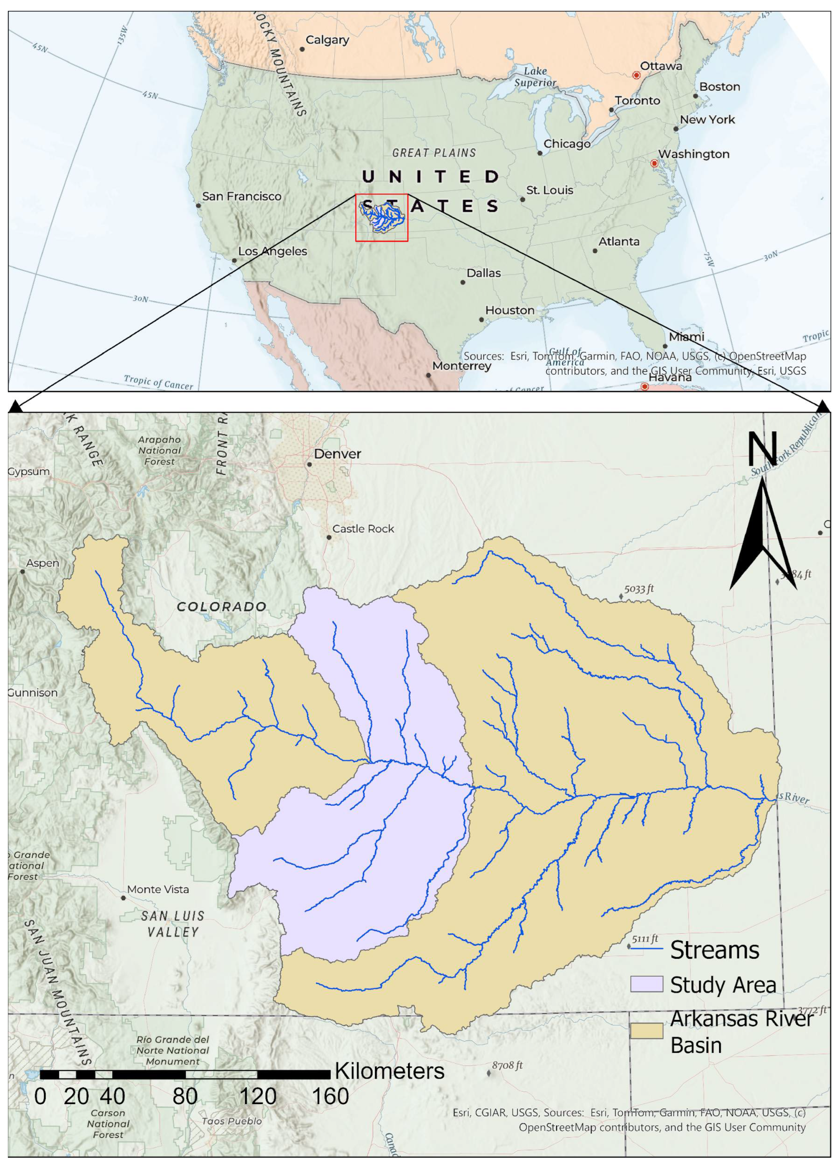
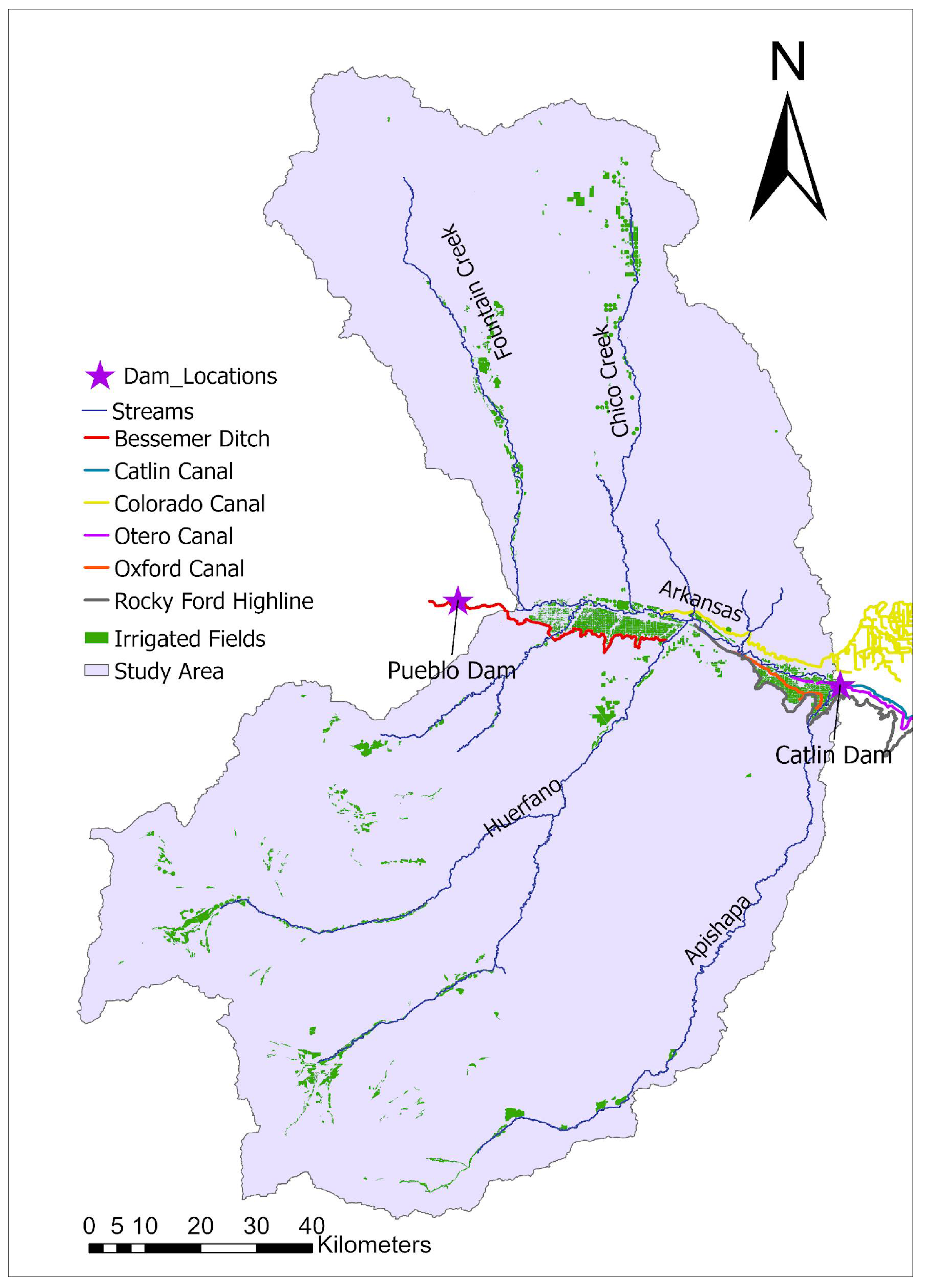
2.1. Study Area

The Arkansas River originates in the Rocky Mountains and flows about 640 km through Colorado, supporting agriculture, municipalities, and industry [35]. Extensive modeling efforts in different sections of this basin have addressed issues like flow and salt transport [36], selenium and nitrogen contaminant dynamics [37,38], salinity [34,39], and groundwater–surface water interactions [40,41]. The study area is approximately a 15,900 km² portion of the Arkansas River Basin in the state of Colorado in the Western USA. Figure 1 displays the location of the study area within the USA (indicated by a red rectangle), along with a zoomed-in view of the Arkansas River Basin highlighting the selected study area. This region experiences a semi-arid climate, receiving an average annual precipitation of roughly 360 mm.

Figure 2 shows the Arkansas River and its tributaries in the study area along with main canals, irrigated fields, and dams. The Arkansas River is primarily fed by snowmelt from the Rocky Mountains, supplemented by precipitation throughout the year, leading to a complex flow pattern with significant seasonal variations. Major tributaries such as Fountain Creek, Huerfano River, and Apishapa contribute to the river’s flow, in addition to the main flow released from the Pueblo Dam. Compared to the mountainous terrain in the upper part of the Arkansas River Basin, this study area is relatively flat.

The total irrigated area in the study area is about 430 km². Infrastructure, such as the Pueblo Dam and various irrigation systems, plays a crucial role in water management in the study area. Excessive irrigation, canal seepage, and inadequate drainage have led to saline shallow groundwater and soil salinity beneath irrigated areas throughout the Arkansas River Valley. This, in turn, has accelerated the subsurface dissolution of naturally occurring salts and selenium, ultimately causing their discharge into the Arkansas River [36,42,43,44]. The selenium [45] and salinity [37,45,46,47] problem aggravated due to irrigation in the region is reported in several studies.

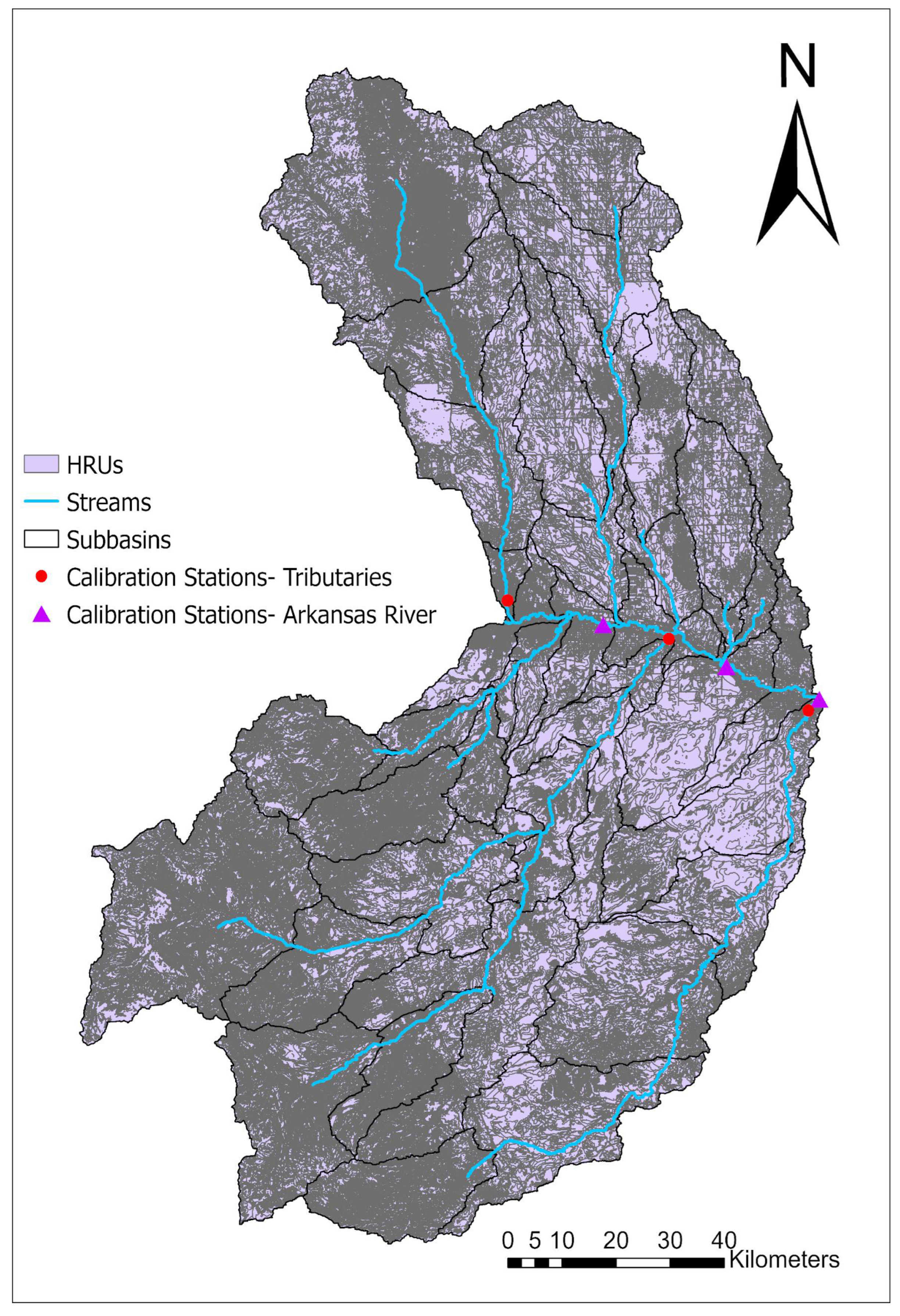
2.2. SWAT Model and Its Setup

SWAT [48] is a hydrologic model that operates at the watershed scale on a daily time step, employing a semi-distributed approach. The watershed is segmented into sub-basins, each containing a stream that facilitates the movement of surface water into another sub-basin [20]. Additionally, each sub-basin is further subdivided into Hydrologic Response Units (HRUs), characterized by unique combinations of soil type, land use, and slope. HRUs, serving as aggregated units within sub-basins, may not necessarily be spatially interconnected. Widely utilized globally, it is particularly known for its effectiveness in modeling both water quality and quantity. The model operates based on the water balance, as outlined in Equation (1) below [20]:

$$\mathrm{SWt}=\mathrm{SWo}+{\sum }_{\mathit{i}=1}^{\mathit{t}}(\mathrm{R}\mathrm{d}\mathrm{a}\mathrm{y}-\mathrm{Q}\mathrm{s}\mathrm{u}\mathrm{r}\mathrm{f}-\mathrm{E}\mathrm{a}-\mathrm{W}\mathrm{s}\mathrm{e}\mathrm{e}\mathrm{p}-\mathrm{Q}\mathrm{g}\mathrm{w})$$

(1)

where

• SWt = Final water content of the soil at any time t;
• SWo = Initial water content of the soil;
• Rday = Daily precipitation;
• Qsurf = Daily surface runoff;
• Ea = Daily evapotranspiration;
• Wseep = Daily percolation;
• Qgw = Daily return flow.

In SWAT, within each sub-basin, a lumped module is used to represent groundwater which is further divided into shallow and deep aquifers. Both the shallow and deep aquifers can discharge into streamflow as baseflow, disregarding distributed parameters such as hydraulic conductivity and storage coefficients [20]. Consequently, this simplification makes it challenging to accurately estimate the groundwater movement in watersheds.

The conventional SWAT model for the study area was developed using the data presented in

Table 1. Input data source and type to SWAT model.

Data	Source	Data Type
Digital Elevation Model DEM	The National Map viewer, USGS DEM, 2010	10 m Grid
Soil Map	Soil Survey Geographic Database (SSURGO), USDA, 2009	Shapefile
Land-use Map	National Agricultural Statistics Service (NASS) USA, 2010	30 m Grid
Precipitation	PRISM database (https://prism.oregonstate.edu/) (5 June 2025)	January 1990–July 2014, Daily
Max-Min Temperature	PRISM database (https://prism.oregonstate.edu/) (5 June 2025)	January 1990–July 2014, Daily
Solar Radiation, Wind Speed, Relative Humidity	CFSR database	January 1990–July 2014, Daily
Streamflow	Colorado Decision Support System (CDSS), USA	Daily Mean observed flow
Canal Diversion	Colorado Decision Support System (CDSS), USA	Daily surface water diversion

. A Digital Elevation Model (DEM) from USGS was employed to delineate streams and sub-basins and to calculate slope in the SWAT model. Inflow data at the USGS streamgage at Moffat Street in Pueblo was used as input for the model. Utilizing the soil map, land-use map, and slope information obtained from the DEM, SWAT created Hydrologic Response Units (HRUs) for the model. Daily weather data, including solar radiation, wind speed, precipitation, relative humidity, and minimum/maximum temperature, was used for the period from 1990 to 2014 to complete the model setup.

Figure 3 below illustrates the study area with sub-basins and HRUs delineated by the SWAT model, including irrigated HRUs, canals, and wells. The Arkansas River flows from west to east, with tributaries joining from both the south and north. The irrigated areas along the Arkansas River indicate that the corridor is heavily irrigated. The model has 44 sub-basins and 28,540 hrus. Purple triangles in Figure 2 show the calibration stations along the Arkansas River: Arkansas River at Avondale, Nepesta, and Catlin Dam; the red dots are the calibration stations along the tributaries: Fountain Creek at Pueblo, Huerfano River, and Apishapa River from upstream to downstream.

2.3. Modification of the SWAT Model

Modifications to the conventional SWAT model for irrigated fields in the study area were implemented using ArcGIS to align HRU boundaries with cultivated field boundaries, following the approach of [38]. This modified HRU definition ensured that each unique HRU corresponded to an individual field. Additionally, adjustments were made to the management operation parameters of HRUs representing the fields, including irrigation settings, based on a database containing crops, irrigation, and fertilizer application data for each field based on the study by [49].

Water diversions from all canals in the area were integrated into the model by designating point sources (withdrawals) at diversion locations, with recorded daily diversion data (Colorado Division of Water Resources; https://cdss.colorado.gov/; accessed on 20 May 2024) used to assign negative inflows equivalent to the diverted amounts. A particular challenge arose because the Bessemer Ditch canal, originating outside the study area, irrigates fields within it, while other canals, such as the Colorado Canal, Oxford Canal, and Rocky Ford Highline, divert water from the Arkansas River within the model area but also transport water beyond it.

To address this and improve water balance estimations, auto-irrigation was assigned to each field in the SWAT model. This approach ensures irrigation occurs whenever crops experience water stress, incorporating the irrigation water used in fields into the water balance while allowing excess water to exit the model system, as occurs in the real system. Fields within a 50 m radius of a well are assigned to a groundwater source from their respective sub-basin aquifers, while other fields receive auto-irrigation from surface water, thereby simulating both surface and aquifer irrigation in the study area.

Seepage from the earthen irrigation canals to the unconfined aquifer is a major groundwater source throughout the irrigated regions. This source was simulated by modifying the SWAT source code to allow for an additional recharge term to the daily groundwater balance equation for each affected aquifer. HRUs intersecting canals were identified and assigned seepage rates of 3.3 × 10⁻⁵ m³/s/m which was an average estimate based on [50] for the days the canals carried water during the modeling period, with the seeped water ultimately contributing to the shallow aquifer. These data are entered into a text file, which is read into the SWAT code at the beginning of the simulation.

2.4. Calibration of the SWAT Model

The SWAT model was calibrated using the Soil and Water Assessment Tool–Calibration and Uncertainty Procedures Sequential Uncertainty Fitting (SWAT CUP—SUFI) which is a tool specifically designed to facilitate the calibration and uncertainty analysis of the Soil and Water Assessment Tool (SWAT) model. SWAT-CUP provides a user-friendly interface that integrates with SWAT to streamline the calibration process and enhance the model’s accuracy and reliability. The parameters for calibration are chosen based on literature review [20,51] and listed in

Table 2. Calibration parameters and calibrated values.

Parameters	Definition	Range of Values		Calibrated Values Irrigated Corridor
		Minimum	Maximum
CN2	SCS runoff curve number for moisture condition II	−30%	+30%	−5.7%
ESCO	Soil evaporation compensation factor	0.01	1.0	0.15
OV_N	Manning’s n value for overland flow	0.005	0.8	0.39
CH_N2	Manning’s n for main channel	0.016	0.15	0.12
CH_K2	Effective hydraulic conductivity of channel (mm/hr)	0.025	140	86.3
SHALLST	Initial depth of water in the shallow aquifer (mm)	0	10,000	843
GW_DELAY	Delay time for aquifer recharge (days)	0.001	100	24
GWQMN	Threshold depth of water level in shallow aquifer for return base flow to occur (mm)	0.01	100	0.01
ALPHA_BF	Base flow recession constant (days)	0.1	1.0	0.75
GW_REVAP	Groundwater ‘revap’ coefficient	0.01	1.0	0.2
REVAPMN	Threshold depth of water level in shallow aquifer for ‘revap’ to occur (mm)	0	1000	1000
SOL_AWC	Available water capacity	−0.5	0.5	−0.06%
SOL_K	Saturated hydraulic conductivity	−0.5	0.5	0%
TIMP	Snowpack temperature lag factor	0.5	1	1
SFTMP	Snowfall temperature (deg C)	−10	5	1
SMFMN	Melt factor for snow on 21 June (mm/deg C-day)	1.4	6.9	4.5
SMFMX	Melt factor for snow on 21 December (mm/deg C-day)	1.4	6.9	4.5
SMTMP	Snow melt base temperature (deg C)	−5	5	0.5
SURLAG	Surface runoff lag time	0.01	12	4

.

Since the watershed is large, and applying the same parameters to all sub-basins resulted in poor model results for the tributaries. To address this, a three-step calibration approach was used. First, the sub-basins contributing to tributaries with available data (Fountain Creek, St. Charles, Huerfano, and Apishapa) were calibrated at the sub-basin scale individually, using the flow data at the outlets of these creeks before they join the Arkansas River. In the second step, the remaining sub-basins were calibrated for flows at the Arkansas River at Avondale, Nepesta, and Catlin Dam. In the third step, the parameters at the basin scale were varied to achieve the best flow results at all four stations in the tributaries and three stations at the Arkansas River. The last column in Table 2 presents the calibrated parameter values for the irrigated corridor, and the parameters for the subwatersheds and watershed scale are presented in

Table A2. Calibrated parameters for the fountain, creek, Huerfano, Apishapa, and watershed scale.

Parameters	Calibrated Values Fountain Creek	Calibrated Values Huerfano	Calibrated Value Apishapa
CN2	−29%	−18%	−18%
ESCO	0.76	0.55	0.55
OV_N	0.15	0.17	0.17
CH_N2	0.15	0.16	0.16
CH_K2	1.9	15	17
SURLAG	4	4	4
SHALLST	7969	127	100
GW_DELAY	7.5	49	25
GWQMN	22.8	55	500
ALPHA_BF	0.9	0.04	0.06
GW_REVAP	0.9	1.0	0.99
REVAPMN	25	500	0.001
SOL_AWC	+0.44%	−0.21	+0.37
SOL_K	−0.23%	+0.3	−0.49
TIMP	1	1	1
SFTMP	1	1	1
SMFMN	4.5	4.5	4.5
SMFMX	0.5	0.5	0.5
SMTMP	4	4	4

. This approach helps assign different parameters at the subwatershed scale, thereby better capturing the variable watershed properties in the study area.

2.5. Wet and Dry Period Analysis and Management Scenarios

The wet and dry years on an annual scale were identified. Anomalies, shown in

Table A1. Wet and dry years in the study area.

Year	Annual Precipitation	Anomaly (Precipitation Average)
1990	352.16	53.83
1991	306.77	8.447083333
1992	302.16	3.837083333
1993	320.3	21.97708333
1994	299.81	1.487083333
1995	313.61	15.28708333
1996	299.09	0.767083333
1997	385.26	86.93708333
1998	317.98	19.65708333
1999	372.9	74.57708333
2000	253.48	−44.84291667
2001	230.37	−67.95291667
2002	162.51	−135.8129167
2003	293.16	−5.162916667
2004	376.13	77.80708333
2005	312.08	13.75708333
2006	321.23	22.90708333
2007	328.35	30.02708333
2008	301.74	3.417083333
2009	318.51	20.18708333
2010	284.64	−13.68291667
2011	256.44	−41.88291667
2012	166.55	−131.7729167
2013	284.52	−13.80291667
Average		294.38 mm
Standard Deviation		57.45

, represent the difference between annual precipitation and the average annual precipitation across the modeling period. Years with anomalies greater than one standard deviation were classified as wet years, while those with anomalies falling below one standard deviation from the mean were classified as dry years. All the years that had precipitation within one standard deviation are considered normal precipitation years. In the table, rows highlighted in blue indicate wet years (1997, 1999, and 2004), while rows highlighted in yellow represent dry years (2001, 2002, and 2012). The year 2014 is excluded because the model only extends to July 2014, and using partial data for anomaly calculation could lead to misleading results.

Six management scenarios were analyzed using the calibrated model: All-Canals, All-Sprinkler, and Canal Sealing at levels of 20%, 40%, 60%, and 80%. In the All-Canals scenario, all fields previously irrigated by 742 wells were reassigned to receive water directly from the stream within their respective sub-basins, eliminating groundwater use. For the All-Sprinkler scenario, management files were adjusted to eliminate surface runoff, simulating full conversion to sprinkler irrigation. In the Canal Sealing scenarios, the seepage rates specified in the “canal.seepage” file were reduced to represent the effects of sealing at each level.

3. Results and Discussions

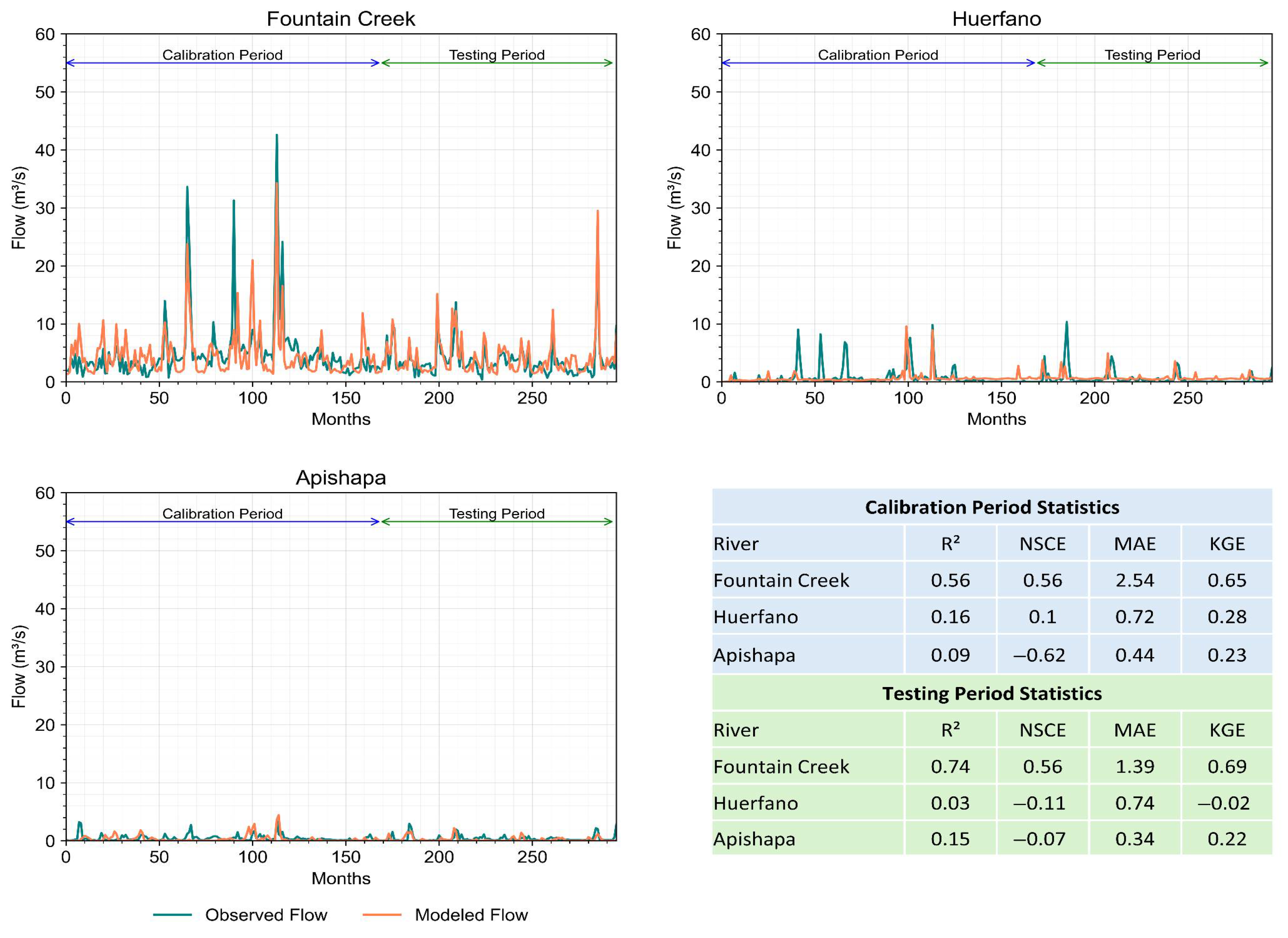
3.1. Streamflow

Figure 4 illustrates the comparison between observed and modeled mean monthly flows at Avondale, Nepesta, and Catlin Dam along the Arkansas River. The x-axis represents the months from January 1990 to July 2014, and the y-axis represents the flows in cubic meters per second (m³/s). The calibration period for the model is from 1990 to 2003, and the testing period is from 2003 to 2014. Goodness of fit (R²), Nash Sutcliffe Coefficient of Efficiency (NSCE), Mean Absolute Error (MAE), and Kling Gupta Efficiency (KGE) show that the model is performing well in both the calibration and testing periods in terms of flow prediction along the Arkansas River.

Figure 5 shows a similar comparison of observed versus modeled flows, with the y-axis representing flows in cubic meters per second (m³/s) and the x-axis representing months, for the tributaries of the Arkansas River: Fountain Creek, Huerfano River, and Apishapa River, measured at the mouth of each tributary. Fountain Creek is the biggest tributary of the Arkansas River in the study area, and the model’s performance is good for Fountain Creek. However, the model does not predict the flow reliably in the Huerfano and Apishapa. But, given the insignificant flows coming in from Huerfano and Apishapa to the Arkansas River, overall model performance is good.

3.2. Streamflow Components and Fluxes in Watershed

Table 3. Average annual flux table for irrigated corridor and watershed and subwatershed scales.

Watershed	PRECIP (mm)	ET (mm)	SURQ (mm)	GWQ (mm)	LATQ (mm)	IRR (mm)	GW Rch (mm)
Fountain Creek	392	376	9	19	18	1	22
Huerfano	393	358	1	0	23	0	18
Apishapa	382	377	2	2	10	1	12
Irrigated Corridor	300	487	72	100	1	224	108
Watershed Scale	359	369	7	14	16	2	25

presents the average annual water fluxes at the watershed scale, within the irrigated corridor, and across the Fountain Creek, Huerfano, and Apishapa subwatersheds. Precipitation varies across the watershed, with the irrigated corridor receiving the least (300 mm). Evapotranspiration (ET) remains relatively consistent among the subwatersheds, ranging from 358 mm in Huerfano to 377 mm in Apishapa. The watershed-scale ET (369 mm) lies within this range. However, the irrigated corridor exhibits a markedly higher ET of 487 mm which reflects the intensive irrigation practices in the area. This region also shows elevated values for surface runoff, soil water, groundwater return flow, and groundwater recharge, likely due to significant irrigation from the Arkansas River via irrigation canals. While irrigation occurs in the subwatersheds as well, its impact on overall water balance appears negligible at the subwatershed scale.

The bar charts in Figure 6 show the water flux happening in the watershed at the subwatershed scales for Apishapa, Huerfano, and Fountain Creek subwatersheds along with the irrigated corridor along the Arkansas River and the whole watershed scale. The y-axis represents groundwater return flow and surface runoff. When comparing the flow components at the same scale in the bar charts, the contributions from Huerfano and Apishapa appear negligible, consistent with the results shown in Figure 5. More than 90% of the water from precipitation is lost to ET in all three subwatersheds as well as at the watershed scale with a tiny fraction of that converting to other flow components. Groundwater return flow to the streams is higher in Fountain Creek compared to the Huerfano and Apishapa.

The pie charts in the top right corner of each bar chart in Figure 6 depict the percent contributions of groundwater return flow, lateral flow, and surface runoff to total streamflow. In the irrigated corridor, groundwater return flow accounts for a substantial portion of streamflow (58%), followed by surface runoff (42%), while lateral flow remains negligible, underscoring the dominance of irrigation-driven aquifer discharge in this region. This finding aligns with studies that show irrigation recharge significantly augments baseflow in irrigated alluvial valleys, particularly where canal seepage and deep percolation elevate local groundwater tables and enhance discharge to nearby streams [52,53].

Similarly, in the Fountain Creek subwatershed, both groundwater (41%) and lateral flow (39%) play major roles, suggesting a more balanced hydrologic regime with substantial contributions from both saturated and unsaturated zone processes. In contrast, the Apishapa and Huerfano subwatersheds exhibit minimal groundwater contributions but high lateral flow dominance, indicative of active water movement through the root zone in less irrigated or upland areas. At the broader watershed scale, streamflow composition—42% lateral flow, 39% groundwater return, and 19% surface runoff—highlights the importance of interflow processes and root zone dynamics in shaping the overall flow regime. These trends are consistent with hydrograph separation studies and recent groundwater modeling efforts that emphasize the delayed but sustained impact of subsurface return flows, particularly in semi-arid irrigated basins of the western USA [54].

A prior study [30] applied the SWAT+ gwflow model to the Arkansas River Basin in Colorado for the period 2000–2015 and reported average annual ET values of 392 mm for the Fountain Creek subwatershed (approximately 91% of total precipitation), 392 mm for Huerfano (about 95%), and 367 mm for Apishapa (about 98%). These correspond to ET-to-precipitation ratios in this study of 93% for Fountain Creek, 92% for Huerfano, and 99% for Apishapa (Table 3). Despite the different simulation periods, 2000–2015 by [30] and 1990–2014 in the current study, the ET estimates are in good agreement, indicating consistency in model performance across timeframes. The estimates of average annual surface runoff and lateral flow by the study in Fountain Creek are 16.7 mm and 11.9 mm by [30], whereas this study reports those values as 7 mm and 16 mm, respectively.

Figure 7 illustrates the average daily seepage (m³/day) across the study area during the modeling period. The highest seepage rates (>50,000 m³/day) are observed along the irrigated corridor of the Arkansas River, where major water diversions occur by the canals shown by red lines, and most irrigated fields are concentrated. The blue lines represent the rivers in the study area. This suggests that the irrigated corridor functions as a significant recharge zone. Refs. [50,55] report seepage through canals in the Arkansas River Basin to be 0.01 to 0.14 m³/s/km of canal length which converts to 864 m³/day to 12,000 m³/day per kilometer length of canal. The discharge rates simulated by the model in this study are comparable to these observed values.

3.3. Wet and Dry Period Analysis

Table 4. Fluxes for wet and dry years in the irrigated corridor.

Years	PRECIP (mm)	PET (mm)	ET (mm)	SURQ (mm)	GWQ (mm)	LATQ (mm)	IRR (mm)	GW Rch (mm)
1997	364	1347	486	70	103	1	218	111
1999	356	1507	505	68	109	1	210	118
2004	410	1477	544	68	109	1	211	117
2001	287	1637	512	78	108	1	246	116
2002	121	1733	369	90	109	1	284	117
2012	161	1620	408	81	109	0	254	115

presents water fluxes for selected wet and dry years in the irrigated corridor, where, as shown in Table 3, water fluxes are most pronounced. The years 1997, 1999, and 2004 are classified as wet years due to higher precipitation, yet evapotranspiration (ET) during these years still exceeds precipitation, likely due to the usage of stored soil water and supplemental irrigation from canal diversions. The irrigated agriculture in practice is helping better crop productivity, adversely absorbing the climate to some extent. In contrast, potential evapotranspiration (PET) is higher during the dry years (e.g., 2001, 2002, 2012), which aligns with reduced atmospheric moisture leading to increased evaporative demand. Despite ongoing irrigation, lower ET values in dry years such as 2002 and 2012 indicate reduced vegetative or crop growth under drought conditions. This suggests that the crops might have experienced reduced growth likely due to extreme heat or limited water availability at critical growth stages.

In the irrigated corridor, the highest precipitation was recorded in 2004 at 410 mm and the lowest precipitation was recorded in the year 2002 at just 121 mm, attributed to the highest and lowest ETs (Table 4). On average, wet years exhibited surface runoff of 69 mm, compared to 83 mm in dry years. Similarly, the average groundwater return flow was 107 mm for wet years and 109 mm for dry years. Groundwater recharge averaged 115 mm in wet years and 116 mm in dry years. The higher values of surface runoff, infiltration, and groundwater return flow during dry years indicate the influence of irrigation water applied during those periods.

Figure 8 and Figure 9 illustrate the temporal patterns of precipitation, evapotranspiration, surface runoff, lateral flow, groundwater return flow, and soil water content in the irrigated corridor (Figure 8) and at the watershed scale (Figure 9). A large portion of precipitation is lost to evapotranspiration or retained as soil water. In Figure 8, surface runoff is observed primarily during wet years in the irrigated corridor, with minimal runoff during dry years. However, groundwater return flow remains relatively constant across both wet and dry years, while its value increases during the growing season, likely due to consistent irrigation supplied by diversions from the Arkansas River via multiple canals.

Even though the monthly distribution of fluxes differs noticeably between wet and dry years at the watershed scale, as shown in Figure 9,

Table 5. Fluxes for wet and dry years in the watershed scale.

Years	PRECIP (mm)	PET (mm)	ET (mm)	SURQ (mm)	GWQ (mm)	LATQ (mm)	IRR (mm)	GW Rch (mm)
1997	506	1264	402	7	15	19	2	23
1999	496	1477	451	11	18	22	2	42
2004	483	1463	440	7	15	21	2	25
2001	339	1534	357	7	15	11	3	26
2002	203	1615	220	7	15	6	3	23
2012	216	1501	261	7	15	10	3	24

indicates that the average surface runoff (8 mm in wet and 7 mm in dry years) and groundwater return flow (16 mm in the wet years vs. 14 mm in the dry years) are not drastically different between the two-year types. In contrast, evapotranspiration (431 mm in wet years vs. 298 mm in dry years) and precipitation (495 mm vs. 266 mm) are significantly higher in wet years.

Higher precipitation at the watershed scale compared to the irrigated corridor indicates spatial variability in rainfall across the basin. At the watershed scale, most of the precipitation is lost to evapotranspiration, and groundwater recharge is higher during wet years than in dry years. However, groundwater discharge remains relatively consistent between wet and dry years, suggesting that recharged groundwater is released gradually and at a relatively steady rate into the stream network. Even though total precipitation is much lower in dry years than in wet years, the average surface runoff is higher in wet years by only about 1 mm. This suggests that the surface runoff generated during precipitation events is relatively small at the watershed scale, but still, higher precipitation tends to produce higher surface runoff at the watershed scale. Irrigation depth, which is a tiny fraction compared to total water in the system, seems to have no effect on the fluxes at the watershed scale.

3.4. Management Scenarios

Table 6. Average annual fluxes and storages in the irrigated corridor (1990–2014).

Parameter	Baseline	All Sprinkler	All Canal	20% Canal Sealing	80% Canal Sealing
Lateral Flow (mm)	1	0	1	1	1
Groundwater Flow (mm)	100	96	100	85	43
Precipitation (mm)	300	300	300	300	300
Surface Runoff (mm)	72	1	72	72	72
Evapotranspiration (mm)	487	486	487	487	487
Groundwater Recharge (mm)	108	41	108	93	46
Irrigation (mm)	224	216	224	224	224

and

Table 7. Average annual fluxes and storages in the watershed (1990–2014).

Parameter	Baseline	All Sprinkler	All Canal	20% Canal Sealing	80% Canal Sealing
Lateral Flow (mm)	16	16	16	16	16
Groundwater Flow (mm)	14	14	14	13	7
Precipitation (mm)	359	359	359	359	359
Surface Runoff (mm)	7	2	7	7	7
Evapotranspiration (mm)	369	370	369	369	369
Groundwater Recharge (mm)	25	24	25	22	14
Irrigation (mm)	3	3	3	3	3

summarize the total fluxes, including lateral flow, groundwater flow, precipitation, snowmelt, surface runoff, evapotranspiration (ET), soil water, groundwater recharge, and irrigation, for each scenario at both the watershed scale and the irrigated corridor. The sprinkler irrigation scenario resulted in a substantial reduction in surface runoff (99%), along with a 62% decrease in groundwater recharge and a 6% reduction in groundwater return flow. Under the 20% and 80% canal sealing scenarios, groundwater recharge and discharge in the irrigated corridor declined by approximately 15% and 60%, respectively. At the watershed scale, however, the fluxes across scenarios remain largely unchanged, consistent with the baseline scenario, indicating that the impacts of these interventions are primarily localized to the irrigated corridor.

3.4.1. All-Canal Scenario

We transformed well-irrigated fields into canal-irrigated fields by reallocating their water source to streams within their respective sub-basins. Figure 10 presents a bar chart illustrating the average monthly fluxes of surface runoff and groundwater return flow, along with the components contributing to surface runoff in the corresponding streams. Comparing the All-Canal Scenario in Figure 10 to the Baseline Scenario in Figure 5 reveals that converting all well-irrigated fields to canal irrigation resulted in almost negligible to no changes in the irrigated corridor, subwatershed, and watershed scales. The wells irrigate approximately 19 km² of the irrigated area, representing only about 4% of the total irrigated area of 432 km². Due to this relatively small proportion of well-irrigated land, converting these fields to surface irrigation in the scenario likely had a negligible impact on the overall water balance.

3.4.2. All-Sprinkler Scenario

We can see in Figure 11 below that much of the fluxes remain unchanged in this scenario for Fountain Creek, Huerfano, and Apishapa subwatersheds, while we can see significant changes in fluxes in the irrigated corridor and the watershed scale. When irrigation is shifted from flood to sprinkler systems, surface runoff, groundwater return flow, and lateral flow all decrease significantly. Because of a sharp decline in surface runoff from 72 mm in the baseline scenario to 1 mm in the sprinkler scenario (Table 6), the proportionate contribution of groundwater return flow to surface water increases from 58% in the baseline scenario to 99% under the sprinkler scenario. But there is also a decline of groundwater return flow from 100 mm in the baseline scenario to 96 mm in the sprinkler scenario. These reductions in surface runoff and groundwater return flow seem to reduce the downstream streamflow, but since the irrigation canals divert the water from the Arkansas River, much of the water is left in the river itself because of the high efficiency of the sprinkler system. Therefore, downstream flow remains unaffected.

Ref. [56] reported that converting from flood to sprinkler irrigation reduced baseflow contributions to the stream by 11%, indicating that the water conserved through sprinkler irrigation would have otherwise contributed to downstream flow as baseflow. Similarly, Ref. [57], in a study conducted in the Lower Arkansas River Valley, observed that reducing irrigation rates led to decreased groundwater recharge and surface runoff, findings that align with the results of the present study.

3.4.3. Canal Sealing Scenarios

As shown in Figure 6, the canal seepage is mostly high along the irrigated corridor of the Arkansas River; in this section, we present the impacts of canal seepage along the irrigated corridor only. Figure 12 presents the trend of canal seepage (m³/d) over the modeling period under different levels of canal sealing (0% to 80%). Canal seepage exhibits a recurring seasonal trend, with peaks occurring annually. This suggests that canal seepage is strongly influenced by seasonal irrigation demands and water availability in the canals. The baseline (0% sealing) scenario has the highest canal seepage. As canal sealing increases (from 20% to 80%), seepage progressively decreases. The 80% sealing scenario (purple line) shows the lowest seepage rates, confirming that sealing canals significantly reduces water loss due to seepage. Each step of increased canal sealing leads to a clear, proportional reduction in seepage. Even partial sealing (e.g., 20% or 40%) leads to noticeable reductions, while higher levels of sealing (60–80%) drastically cut seepage losses. As shown in Table 7, groundwater return flow in the irrigated corridor decreases significantly from 108 mm under baseline conditions to 46 mm with 80% canal sealing—nearly a 60% reduction in its contribution to streamflow. However, since irrigation water is primarily diverted from the Arkansas River, with a flow that is regulated by the Pueblo Reservoir just upstream of the study area, most of this seepage source is the upstream release. With canal sealing, less water is needed to offset seepage losses, allowing the reservoir to retain and release that water later to support the flow in the river that would usually come as groundwater return flow from the irrigated corridor. As a result, downstream flows remain largely unaffected despite reduced groundwater return flow within the corridor.

There is a linear relationship between canal sealing and groundwater flow reduction (Figure 13). As the percent of canal sealing increases, the reduction in groundwater flow also increases proportionally. The irrigated corridor shows a slightly greater reduction in groundwater flow compared to the watershed scale for the same level of canal sealing.

3.4.4. Scenario Analysis Results in Wet and Dry Years

From Table 4, Table 5, Table 6 and Table 7 presented above, significant flux is happening in the irrigated corridor of the study region compared to the other regions. In

Table 8. Groundwater recharge (GW_RCH), surface runoff (SURQ), lateral flow (LATQ), and groundwater return flows (GWQ) in mm during dry and wet years under 80% and 20% canal sealing scenarios and sprinkler scenario for the irrigated corridor.

Years	Canal Sealing 80%				Canal Sealing 20%				Sprinkler Scenario
	GW_RCH	SURQ	LATQ	GWQ	GW_RCH	SURQ	LATQ	GWQ	GW_RCH	SURQ	LATQ	GWQ
1997	46	70	1	43	95	70	1	88	108	1	0	100
1999	53	68	1	49	102	68	1	93	113	1	1	103
2004	52	68	1	49	101	68	1	94	113	1	1	105
2001	51	78	1	49	100	78	1	93	111	1	0	103
2002	52	90	1	50	101	90	1	94	113	0	0	105
2012	49	81	0	47	98	81	0	91	111	0	0	103

below, we present the groundwater recharge (GW_RCH), surface runoff (SURQ), lateral flow (LATQ), and groundwater discharge (GWQ) under three different management scenarios in the irrigated corridor under the wet years (1997, 1999, 2004) and dry years (2001, 2002, 2012). The analysis highlights how each scenario affects the water budget, particularly in the context of precipitation variability.

During the wet years, groundwater recharge decreases progressively from sprinkler to canal sealing 20% and canal sealing 80 percent. For instance, in 1999, it decreased from 113 mm in the sprinkler scenario to 53 mm in the 80% sealing scenario. This suggests that canal lining can significantly reduce the groundwater recharge. Surface runoff remains unchanged between the canal sealing scenarios but drops drastically under the sprinkler scenario to just 1 mm. This dramatic reduction indicates that surface runoff during the wet years is primarily driven by irrigation excess, which can be effectively controlled by precision application through sprinklers. Lateral flow is minimal and remains constant across all the scenarios and years, suggesting that it is not a major component of streamflow in this system. Groundwater return flow follows a similar trend to recharge, increasing under improved irrigation methods. For example, in 2004, the groundwater return flow in the sprinkler scenario is 105 mm which reduces to 94 mm in the 20 percent canal sealing and 49 mm under the 80 percent canal sealing scenario. This highlights the role of improved management practices in subsurface water movements.

In dry years, the same general trend persists, although the contrasts become more pronounced due to limited precipitation. Groundwater recharge again decreases under canal sealing scenarios like in the wet years. Surface runoff, which is higher in dry years under flood irrigation (78 to 90 mm), drops to nearly zero under sprinklers. It confirms that the surface runoff in the dry years is primarily irrigation-induced rather than precipitation-driven, and that sprinkler irrigation can effectively eliminate this loss. Groundwater return flow also decreases significantly under canal sealing scenarios (47 mm for 80% canal sealing, 91 mm for 20% canal sealing) compared to 103 mm under the sprinkler scenario without canal sealing.

4. Summary and Conclusions

In this study, we analyzed the hydrological processes within the study area using a modified SWAT model, focusing on the influence of tributaries and irrigation on the Arkansas River. We assessed the region’s hydrology during both wet and dry years and evaluated the effects of converting canal irrigation to sprinkler systems, sealing canals, and shifting from aquifer irrigation to canal-based irrigation. The conclusions of this study are listed below:

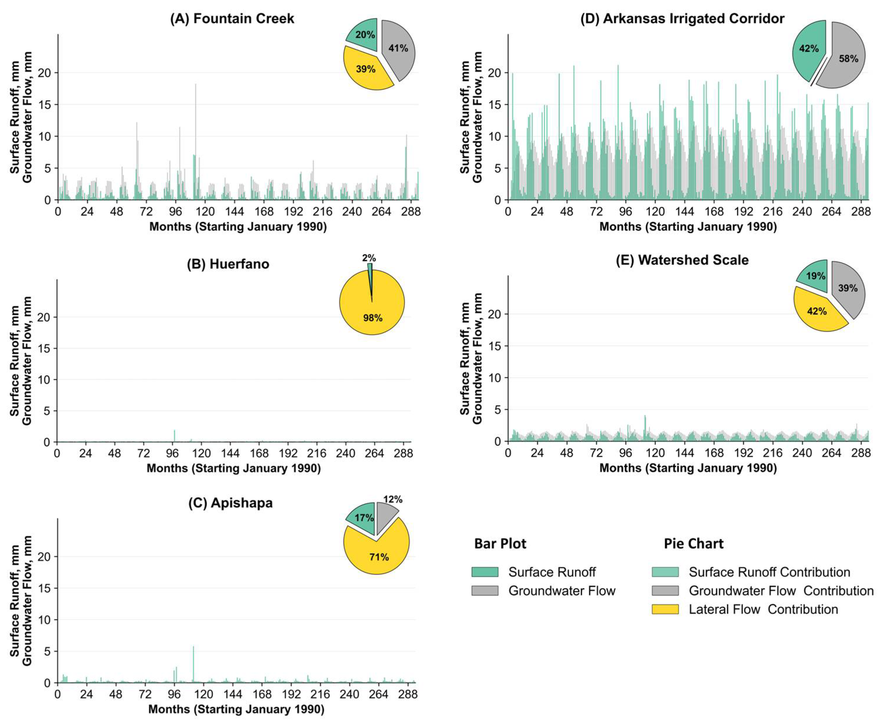
• Over 90% of precipitation in all regions is lost to ET, with limited conversion to other flow components. The irrigated corridor receives the least precipitation (300 mm) but has the highest evapotranspiration (487 mm) and elevated values of surface runoff, soil water, groundwater return flow, groundwater recharge, and canal seepage attributed to irrigation diversions from the Arkansas River. In contrast, the subwatersheds of Fountain Creek, Huerfano, and Apishapa show relatively consistent ET (358–376 mm) and minimal contributions from surface runoff and groundwater return flow.
• The wet and dry year analysis reveals that ET in the irrigated corridor consistently exceeds precipitation, reaching 544 mm in the wet year 2004 despite only 410 mm of rainfall, highlighting the role of irrigation. In dry years like 2002, with just 121 mm of precipitation, surface runoff (90 mm) and groundwater return flow (109 mm) remained high, driven by continued flood irrigation using canals. Compared to the broader watershed, where groundwater return flow averaged only 15 mm across both the wet and dry periods, the irrigated corridor exhibited values almost seven times higher. ET also dropped significantly at the watershed scale from 431 mm in wet years to 279 mm in dry years, indicating drought-induced stress outside irrigated zones. These trends emphasize how irrigation sustains hydrological processes during dry periods and amplifies flow components beyond natural precipitation inputs.
• In the sprinkler irrigation scenario, significant changes in water fluxes occur mainly in the irrigated corridor, where surface runoff drops from 72 mm to 1 mm under sprinkler irrigation, increasing groundwater return flow’s share of streamflow from 58% to 99%, despite a slight decrease in its volume (100 mm to 96 mm). While both runoff and return flow decline, the high efficiency of sprinklers needs to divert less water in canals from the Arkansas River, maintaining downstream flow.
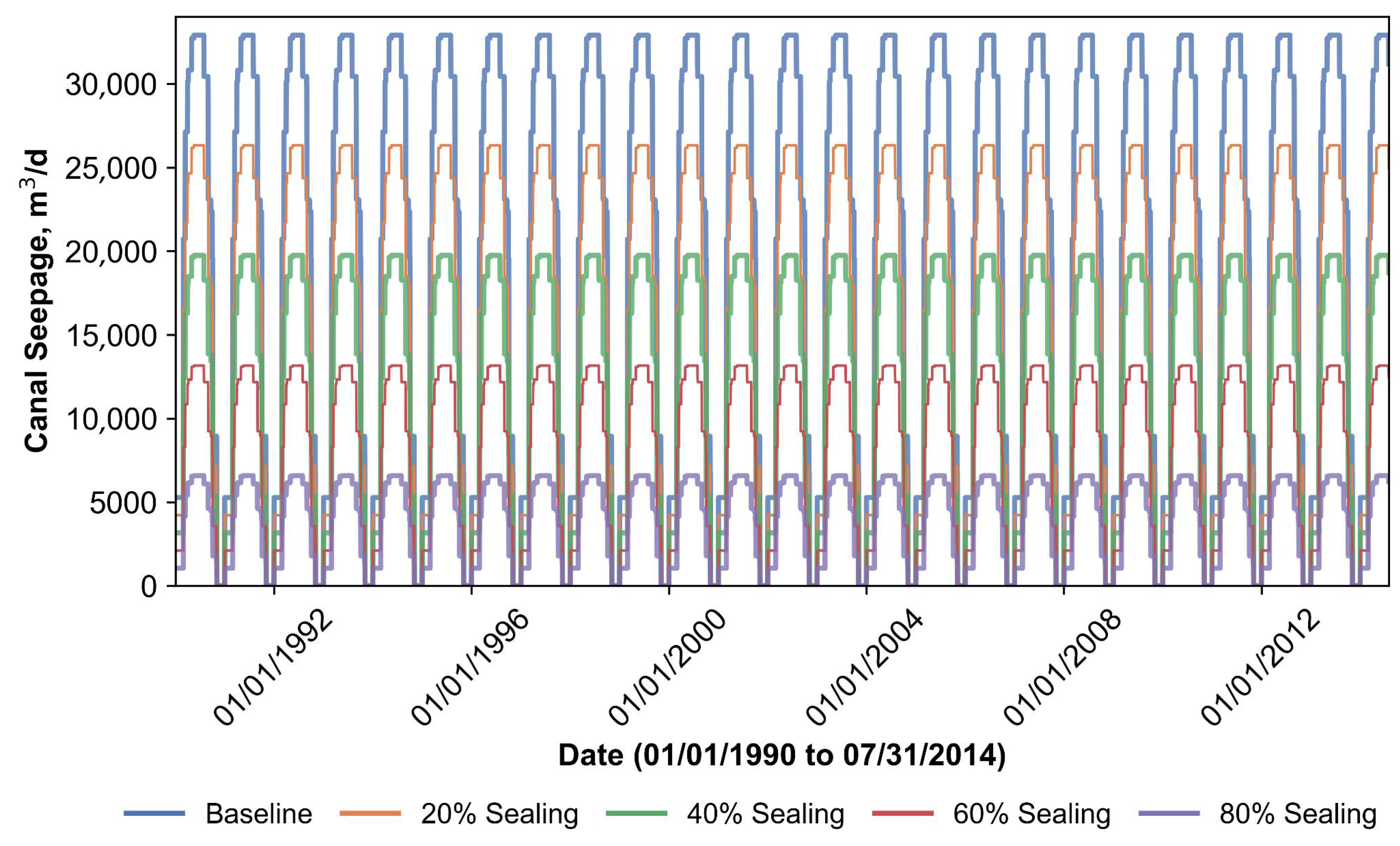
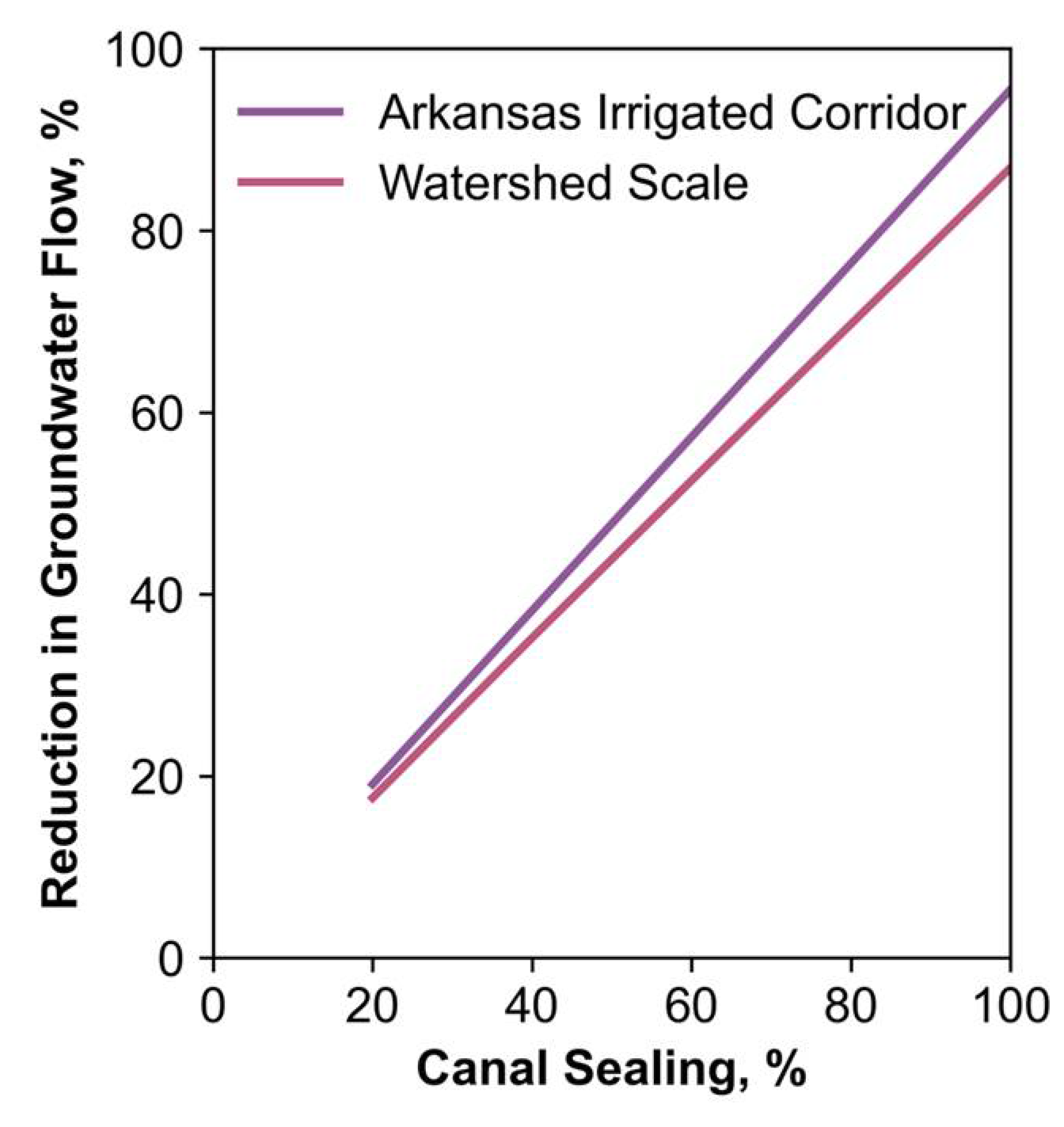
• Canal seepage along the irrigated corridor shows strong seasonal peaks driven by irrigation demand, with the highest seepage under the baseline (0% sealing) condition. As canal sealing increases from 20% to 80%, seepage rates drop proportionally, with the 80% sealing scenario showing the lowest losses. Groundwater return flow in the irrigated corridor decreases sharply from 100 mm in the baseline to 43 mm at 80% sealing—nearly a 60% reduction.
• This study demonstrates that in semi-arid basins, where water resources are increasingly under pressure, improved irrigation management, such as transitioning from canal to sprinkler systems and sealing canals, can significantly reduce non-beneficial water losses while maintaining downstream flows. The substantial reductions in surface runoff and canal seepage under improved management scenarios suggest clear opportunities to decrease overall water demand. By incorporating wet and dry year analyses and evaluating multiple management strategies, this study provides a practical framework that can be applied to similar semi-arid basins worldwide to support sustainable water use under changing climate and resource constraints.

References

1. Qader, S.H.; Dash, J.; Alegana, V.A.; Khwarahm, N.R.; Tatem, A.J.; Atkinson, P.M. The Role of Earth Observation in Achieving Sustainable Agricultural Production in Arid and Semi-Arid Regions of the World. Remote Sens. 2021, 13, 3382. [Google Scholar] [CrossRef]
2. Morante-Carballo, F.; Montalván-Burbano, N.; Quiñonez-Barzola, X.; Jaya-Montalvo, M.; Carrión-Mero, P. What Do We Know about Water Scarcity in Semi-Arid Zones? A Global Analysis and Research Trends. Water 2022, 14, 2685. [Google Scholar] [CrossRef]
3. Pontius, J.; McIntosh, A. Water Scarcity. In Environmental Problem Solving in an Age of Climate Change; Springer textbooks in earth sciences, geography and environment; Springer International Publishing: Cham, Switzerland, 2024; Volume 1, pp. 87–103. [Google Scholar]
4. Mahmoud, M.I.; Gupta, H.V.; Rajagopal, S. Scenario development for water resources planning and watershed management: Methodology and semi-arid region case study. Environ. Model. Softw. 2011, 26, 873–885. [Google Scholar] [CrossRef]
5. Batchelor, C.H.; Rama Mohan Rao, M.S.; Manohar Rao, S.; Batchelor, C.H.; Rama Mohan Rao, M.S.; Manohar Rao, S. Watershed development: A solution to water shortages in semi-arid India or part of the problem? Land Use Water Resour. Res. 2003, 3, 1–10. [Google Scholar]
6. Dehghanisanij, H.; Oweis, T.; Qureshi, A.S. Agricultural water use and management in arid and semi-arid areas: Current situation and measures for improvement. Ann. Arid Zone 2006, 45, 355. [Google Scholar]
7. López-Lambraño, A.A.; Martínez-Acosta, L.; Gámez-Balmaceda, E.; Medrano-Barboza, J.P.; Remolina López, J.F.; López-Ramos, A. Supply and Demand Analysis of Water Resources. Case Study: Irrigation Water Demand in a Semi-Arid Zone in Mexico. Agriculture 2020, 10, 333. [Google Scholar] [CrossRef]
8. Fernández García, I.; Lecina, S.; Ruiz-Sánchez, M.C.; Vera, J.; Conejero, W.; Conesa, M.R.; Domínguez, A.; Pardo, J.J.; Léllis, B.C.; Montesinos, P. Trends and Challenges in Irrigation Scheduling in the Semi-Arid Area of Spain. Water 2020, 12, 785. [Google Scholar] [CrossRef]
9. Lotfirad, M.; Mahmoudi, M.; Esmaeili-Gisavandani, H.; Adib, A. Allocation of water resources with management approaches and under climate change scenarios in an arid and semi-arid watershed (study area: Hablehroud watershed in Iran). Appl. Water Sci. 2025, 15, 74. [Google Scholar] [CrossRef]
10. Nikolaou, G.; Neocleous, D.; Christou, A.; Kitta, E.; Katsoulas, N. Implementing Sustainable Irrigation in Water-Scarce Regions under the Impact of Climate Change. Agronomy 2020, 10, 1120. [Google Scholar] [CrossRef]
11. Sikka, A.K.; Alam, M.F.; Mandave, V. Agricultural water management practices to improve the climate resilience of irrigated agriculture in India. Irrig. Drain 2022, 71, 7–26. [Google Scholar] [CrossRef]
12. Tedeschi, A.; Beltrán, A.; Aragüés, R. Irrigation management and hydrosalinity balance in a semi-arid area of the middle Ebro river basin (Spain). Agric. Water Manag. 2001, 49, 31–50. [Google Scholar] [CrossRef]
13. Zanchi, C.; Cecchi, S. Soil Salinisation in the Grosseto Plain (Maremma, Italy): An Environmental and Socio-Economic Analysis of the Impact on the Agro-Ecosystem. In Coastal Water Bodies; Scapini, F., Ciampi, G., Eds.; Springer: Dordrecht, The Netherlands, 2010; pp. 79–90. [Google Scholar]
14. Minhas, P.S.; Ramos, T.B.; Ben-Gal, A.; Pereira, L.S. Coping with salinity in irrigated agriculture: Crop evapotranspiration and water management issues. Agric. Water Manag. 2020, 227, 105832. [Google Scholar] [CrossRef]
15. Wichelns, D.; Qadir, M. Achieving sustainable irrigation requires effective management of salts, soil salinity, and shallow groundwater. Agric. Water Manag. 2015, 157, 31–38. [Google Scholar] [CrossRef]
16. Fernald, A.G.; Guldan, S.J. Surface water–groundwater interactions between irrigation ditches, alluvial aquifers, and streams. Rev. Fish. Sci. 2006, 14, 79–89. [Google Scholar] [CrossRef]
17. Zhu, J.; Pohlmann, K. Effective approach to calculate groundwater return flow to a river from irrigation areas. J. Irrig. Drain. Eng. 2014, 140, 04013025. [Google Scholar] [CrossRef]
18. Venn, B.J.; Johnson, D.W.; Pochop, L.O. Hydrologic Impacts due to Changes in Conveyance and Conversion from Flood to Sprinkler Irrigation Practices. J. Irrig. Drain Eng. 2004, 130, 192–200. [Google Scholar] [CrossRef]
19. Mashaly, A.F.; Fernald, A.G. Identifying capabilities and potentials of system dynamics in hydrology and water resources as a promising modeling approach for water management. Water 2020, 12, 1432. [Google Scholar] [CrossRef]
20. Neitsch, S.L.; Arnold, J.G.; Kiniry, J.R.; Williams, J.R. Soil & Water Assessment Tool Theoretical Documentation Version 2009; Texas Water Resources Institute: Dallas, TX, USA, 2011. [Google Scholar]
21. Akoko, G.; Le, T.H.; Gomi, T.; Kato, T. A review of SWAT model application in africa. Water 2021, 13, 1313. [Google Scholar] [CrossRef]
22. Tan, M.L.; Gassman, P.W.; Srinivasan, R.; Arnold, J.G.; Yang, X. A review of SWAT studies in southeast asia: Applications, challenges and future directions. Water 2019, 11, 914. [Google Scholar] [CrossRef]
23. Dubey, S.K.; Kim, J.; Her, Y.; Sharma, D.; Jeong, H. Hydroclimatic impact assessment using the SWAT model in india—State of the art review. Sustainability 2023, 15, 15779. [Google Scholar] [CrossRef]
24. Ferraz, L.L.; Santana, G.M.; de Sousa, L.F.; da Silva Amorim, J.; Santos, C.A.S.; de Jesus, R.M. Databases and applications of the soil and water assessment tool (SWAT) model in brazilian river basins: A review. Environ. Model. Assess. 2025, 30, 349–367. [Google Scholar] [CrossRef]
25. Mao, W.; Zhu, Y.; Wu, J.; Ye, M.; Yang, J. Evaluation of effects of limited irrigation on regional-scale water movement and salt accumulation in arid agricultural areas. Agric. Water Manag. 2022, 262, 107398. [Google Scholar] [CrossRef]
26. Huang, S.; Krysanova, V.; Zhai, J.; Su, B. Impact of Intensive Irrigation Activities on River Discharge Under Agricultural Scenarios in the Semi-Arid Aksu River Basin, Northwest China. Water Resour. Manag. 2015, 29, 945–959. [Google Scholar] [CrossRef]
27. Törnqvist, R.; Jarsjö, J. Water Savings Through Improved Irrigation Techniques: Basin-Scale Quantification in Semi-Arid Environments. Water Resour. Manage. 2012, 26, 949–962. [Google Scholar] [CrossRef]
28. Bjorneberg, D.L.; King, B.A.; Koehn, A.C. Watershed water balance changes as furrow irrigation is converted to sprinkler irrigation in an arid region. J. Soil Water Conserv. 2020, 75, 254–262. [Google Scholar] [CrossRef]
29. Wu, X.; Zhou, J.; Wang, H.; Li, Y.; Zhong, B. Evaluation of irrigation water use efficiency using remote sensing in the middle reach of the Heihe river, in the semi-arid Northwestern China. Hydrol. Process. 2015, 29, 2243–2257. [Google Scholar] [CrossRef]
30. Abbas, S.A.; Bailey, R.T.; Arnold, J.G.; White, M.J.; Mirchi, A. Modeling agro-hydrological surface-subsurface processes in a semi-arid, intensively irrigated river basin. J. Hydrol. Reg. Stud. 2025, 57, 102188. [Google Scholar] [CrossRef]
31. Tian, Y.; Zheng, Y.; Wu, B.; Wu, X.; Liu, J.; Zheng, C. Modeling surface water-groundwater interaction in arid and semi-arid regions with intensive agriculture. Environ. Model. Softw. 2015, 63, 170–184. [Google Scholar] [CrossRef]
32. Rahimpour, M.; Tajbakhsh, M.; Memarian, H.; Aghakhani Afshar, A. Impact assessment of climate change on hydro-climatic conditions of arid and semi-arid watersheds (case study: Zoshk-Abardeh watershed, Iran). J. Water Clim. Change 2021, 12, 580–595. [Google Scholar] [CrossRef]
33. Hu, Z.; Wang, L.; Wang, Z.; Hong, Y.; Zheng, H. Quantitative assessment of climate and human impacts on surface water resources in a typical semi-arid watershed in the middle reaches of the Yellow River from 1985 to 2006. Int. J. Climatol. 2015, 35, 97–113. [Google Scholar] [CrossRef]
34. Wei, X.; Bailey, R.T.; Tasdighi, A. Using the SWAT model in intensively managed irrigated watersheds: Model modification and application. J. Hydrol. Eng. 2018, 23, 04018044. [Google Scholar] [CrossRef]
35. Abbott, P.O. Description of water-systems operations in the Arkansas River Basin, Colorado. Water-Resour. Investig. Rep. 1985, 85, 4092. [Google Scholar]
36. Garcia, L.A.; Gates, T.K.; Labadie, J.W. Toward Optimal Water Management in Colorado’s Lower Arkansas River Valley: Monitoring and Modeling to Enhance Agriculture and Environment; Colorado Water Resources Research Institute: Fort Collins, CO, USA, 2006. [Google Scholar]
37. Triana, E.; Labadie, J.W.; Gates, T.K. River GeoDSS for agroenvironmental enhancement of Colorado’s Lower Arkansas River Basin. I: Model development and calibration. J. Water Resour. Plan. Manag. 2010, 136, 177–189. [Google Scholar]
38. Neupane, P.; Bailey, R.T.; Tavakoli-Kivi, S. Assessing controls on selenium fate and transport in watersheds using the SWAT model. Sci. Total Environ. 2020, 738, 140318. [Google Scholar] [CrossRef] [PubMed]
39. Bern, C.R.; Holmberg, M.J.; Kisfalusi, Z.D. Salt flushing, salt storage, and controls on selenium and uranium: A 31-year mass-balance analysis of an irrigated, semiarid valley. J. Am. Water Resour. Assoc. 2020, 56, 647–668. [Google Scholar] [CrossRef]
40. Koehn, W.J.; Tucker-Kulesza, S.E.; Steward, D.R. Conceptualizing Groundwater-Surface Water Interactions within the Ogallala Aquifer Region using Electrical Resistivity Imaging. JEEG 2019, 24, 185–199. [Google Scholar] [CrossRef]
41. Rohmat, F.I.W.; Labadie, J.W.; Gates, T.K. Deep learning for compute-efficient modeling of BMP impacts on stream-aquifer exchange and water law compliance in an irrigated river basin. Environ. Model. Softw. 2019, 122, 104529. [Google Scholar] [CrossRef]
42. Bailey, R.T.; Hunter, W.J.; Gates, T.K. The influence of nitrate on selenium in irrigated agricultural groundwater systems. J. Environ. Qual. 2012, 41, 783–792. [Google Scholar] [CrossRef] [PubMed]
43. Bailey, R.T.; Gates, T.K.; Halvorson, A.D. Simulating variably-saturated reactive transport of selenium and nitrogen in agricultural groundwater systems. J. Contam. Hydrol. 2013, 149, 27–45. [Google Scholar] [CrossRef] [PubMed]
44. Bailey, R.T.; Romero, E.C.; Gates, T.K. Assessing best management practices for remediation of selenium loading in groundwater to streams in an irrigated region. J. Hydrol. 2015, 521, 341–359. [Google Scholar] [CrossRef]
45. Gates, T.K.; Cody, B.M.; Donnelly, J.P.; Herting, A.W.; Bailey, R.T.; Mueller Price, J. Assessing selenium contamination in the irrigated stream-aquifer system of the Arkansas River, Colorado. J. Environ. Qual. 2009, 38, 2344–2356. [Google Scholar] [CrossRef] [PubMed]
46. Goff, K.; Lewis, M.E.; Person, M.A.; Konikowd, L.F. Simulated effects of irrigation on salinity in the arkansas river valley in colorado. Groundwater 1998, 36, 76–86. [Google Scholar] [CrossRef]
47. Brown, A.J.; Andales, A.A.; Gates, T.K. Spatially refined salinity hazard analysis in gypsum-affected irrigated soils. Agrosyst. Geosci. Environ. 2024, 7, e20539. [Google Scholar] [CrossRef]
48. Arnold, J.G.; Srinivasan, R.; Muttiah, R.S.; Williams, J.R. Large area hydrologic modeling and assessment part i: Model development. J. Am. Water Resour. Assoc. 1998, 34, 73–89. [Google Scholar] [CrossRef]
49. Gates, T.K.; Garcia, L.A.; Hemphill, R.A.; Morway, E.D.; Alhaddad, A. Irrigation Practices, Water Consumption, & Return Flows in Colorado’s Lower Arkansas River Valley. Color. Water Inst. Tech. Comp. 2012, 221, 115. [Google Scholar]
50. Susfalk, R.; Sada, D.; Martin, C.A.; Young, M.; Gates, T.K.; Rosamond, C.; Mihevc, T.; Arrowood, T.; Shanafield, M.; Epstein, B. Evaluation of Linear Anionic Polyacrylamide (LA-PAM) Application to Water Delivery Canals for Seepage Reduction; DHS Publication: Las Vegas, NV, USA, 2008; Volume 41245. [Google Scholar]
51. Wallace, C.W.; Flanagan, D.C.; Engel, B.A. Evaluating the effects of watershed size on SWAT calibration. Water 2018, 10, 898. [Google Scholar] [CrossRef]
52. Ferencz, S.B.; Tidwell, V.C. Physical controls on irrigation return flow contributions to stream flow in irrigated alluvial valleys. Front. Water 2022, 4, 828099. [Google Scholar] [CrossRef]
53. Ketchum, D.; Hoylman, Z.H.; Huntington, J.; Brinkerhoff, D.; Jencso, K.G. Irrigation intensification impacts sustainability of streamflow in the Western United States. Commun. Earth Environ. 2023, 4, 479. [Google Scholar] [CrossRef]
54. Gordon, B.L.; Paige, G.B.; Miller, S.N.; Claes, N.; Parsekian, A.D. Field scale quantification indicates potential for variability in return flows from flood irrigation in the high altitude western US. Agric. Water Manag. 2020, 232, 106062. [Google Scholar] [CrossRef]
55. Lund, A.A.R.; Gates, T.K.; Scalia, J. Characterization and control of irrigation canal seepage losses: A review and perspective focused on field data. Agric. Water Manag. 2023, 289, 108516. [Google Scholar] [CrossRef]
56. Ahmadzadeh, H.; Morid, S.; Delavar, M.; Srinivasan, R. Using the SWAT model to assess the impacts of changing irrigation from surface to pressurized systems on water productivity and water saving in the Zarrineh Rud catchment. Agric. Water Manag. 2016, 175, 15–28. [Google Scholar] [CrossRef]
57. Wei, X.; Bailey, R.T. Assessment of System Responses in Intensively Irrigated Stream–Aquifer Systems Using SWAT-MODFLOW. Water 2019, 11, 1576. [Google Scholar] [CrossRef]
Figure 1. Study area within the USA and location of Arkansas River basin with streams.
Geosciences 15 00272 g001
Figure 2. Rivers, main canals, irrigated fields, and dams within the study area.
Geosciences 15 00272 g002
Figure 3. Sub-basins, HRUs, and calibration \stations within the study area.
Geosciences 15 00272 g003
Figure 4. Observed vs. modeled flows along Arkansas River.
Geosciences 15 00272 g004
Figure 5. Observed vs. modeled flows in the tributaries of the Arkansas River.
Geosciences 15 00272 g005
Figure 6. Components of fluxes in sub-basins (bar charts) and streams (pie charts).
Geosciences 15 00272 g006
Figure 7. Average daily canal seepage by sub-basins.
Geosciences 15 00272 g007
Figure 8. Wet and dry year flux analysis in the irrigated corridor.
Geosciences 15 00272 g008
Figure 9. Wet/dry year analysis at the watershed scale.
Geosciences 15 00272 g009
Figure 10. Components of fluxes in sub-basins (bar charts) and streams (pie charts) in All-Canal Scenario.
Geosciences 15 00272 g010
Figure 11. Components of fluxes in sub-basins (bar charts) and streams (pie charts) in All-Sprinkler Scenario.
Geosciences 15 00272 g011
Figure 12. Seepage of irrigation water from the canals under different sealing conditions.
Geosciences 15 00272 g012
Figure 13. Relationship of canal sealing to groundwater flow.
Geosciences 15 00272 g013