Evaluating Time Series Models for Monthly Rainfall Forecasting in Arid Regions: Insights from Tamanghasset (1953–2021), Southern Algeria

Abstract

Accurate precipitation forecasting remains a critical challenge due to the nonlinear and multifactorial nature of rainfall dynamics. This is particularly important in arid regions like Tamanghasset, where precipitation is the primary driver of agricultural viability and water resource management. This study evaluates the performance of several time series models for monthly rainfall prediction, including the autoregressive integrated moving average (ARIMA), Exponential Smoothing State Space Model (ETS), Seasonal and Trend decomposition using Loess with ETS (STL-ETS), Trigonometric Box–Cox transform with ARMA errors, Trend and Seasonal components (TBATS), and neural network autoregressive (NNAR) models. Historical monthly precipitation data from 1953 to 2020 were used to train and test the models, with lagged observations serving as input features. Among the approaches considered, the NNAR model exhibited superior performance, as indicated by uncorrelated residuals and enhanced forecast accuracy. This suggests that NNAR effectively captures the nonlinear temporal patterns inherent in the precipitation series. Based on the best-performing model, rainfall was projected for the year 2021, providing actionable insights for regional hydrological and agricultural planning. The results highlight the relevance of neural network-based time series models for climate forecasting in data-scarce, climate-sensitive regions.

1. Introduction

Water is an indispensable element for sustainability and particularly for water supply and rainfed agriculture, which mostly depends on natural rainfall for crop irrigation. In adults, it constitutes approximately 60% of a human’s body weight, playing an essential role in vital physiological functions such as cellular metabolism, thermoregulation, and tissue lubrication. Beyond its biological significance, water is integral to daily human activities, including washing, cleaning, and cooking [1]. What sets Earth apart from other known celestial bodies is the abundance of liquid water on its surface, covering about 71% of the planet. This extensive presence of water supports a complex web of life, from marine ecosystems to terrestrial habitats, and drives essential biogeochemical cycles [2]. Despite this apparent abundance, the availability of freshwater suitable for human consumption is limited and unevenly distributed [3]. Challenges such as climate change, population growth, and increased demand exacerbate water scarcity issues, underscoring the urgent need for sustainable and equitable water resource management. Preserving this vital resource is imperative to ensure the survival and prosperity of future generations [4,5,6].

Effective management of water resources, which involves the planning, preservation, and enhancement of both their quality and quantity, is vital to meet increasing domestic, agricultural, and industrial demands [7,8,9]. Moreover, it plays a pivotal role in mitigating the impacts of extreme hydrological events such as floods [10,11,12].

However, water scarcity remains a profound challenge, particularly in arid and semi-arid regions where limited and unpredictable precipitation severely disrupts ecological balance and socioeconomic development [13]. Precipitation variability, in both spatial and temporal dimensions, exerts a significant influence on hydrological systems, agriculture, and the overall climate [14,15].

Accurate precipitation measurement is, therefore, essential for understanding these impacts and for managing water resources effectively [16]. Although ground-based rain gauges provide the most accurate data, their sparse and uneven distribution [17,18], particularly in the South Mediterranean region, including Algeria, introduces substantial spatial uncertainties. Rather than focusing solely on the spatial continuity of rainfall data, it is important to emphasize the need for accurate temporal forecasting methods. In regions with limited observational coverage, traditional approaches often struggle to capture the timing and intensity of rainfall events [19]. Therefore, time series-based forecasting models have become essential tools to predict rainfall dynamics and support early warning systems, especially in arid and semi-arid areas where precipitation is both scarce and highly variable [20]. This perspective justifies the use of time series models as a complementary solution to existing measurement networks, providing a means to anticipate rainfall evolution over time in data-scarce environments [21]

In this context, time series modeling has become an indispensable approach for anticipating rainfall variability in data-scarce and climatically sensitive regions [22,23]. Unlike static climatological analyses, time series models allow the extraction of temporal patterns such as trends, cycles, and seasonal fluctuations that are important for understanding rainfall behavior over time. Classical statistical models like ARIMA (autoregressive integrated moving average) and exponential smoothing methods (ETS) have proven effective in linear systems with stable seasonality, while more recent approaches such as TBATS and NNAR (neural network autoregressive) can handle complex, nonlinear, and non-stationary rainfall dynamics [24]. These models are especially useful in regions like Tamanghasset, where precipitation events are irregular, sparse, and often extreme [25]. The ability to generate short- and medium-term forecasts based on historical rainfall records makes time series modeling a powerful decision-support tool for early warning systems, agricultural planning, and integrated water resource management [26]. Furthermore, combining time series models with machine learning algorithms can significantly improve forecast reliability, offering a pathway toward adaptive climate resilience strategies in arid and semi-arid zones. Beyond rainfall forecasting, numerous recent studies have also highlighted the crucial contribution of geostatistical approaches and machine learning in assessing aquifer vulnerability and modeling the geochemical evolution of groundwater, particularly in arid regions where anthropogenic and climatic pressures are compounded [27,28].

The Tamanghasset region in southern Algeria vividly illustrates the consequences of chronic water scarcity. With groundwater reservoirs—the principal sources of supply— showing significant declines, the region faces mounting pressure on its already limited water resources [29]. Shared aquifers with neighboring countries such as Libya and Tunisia further exacerbate the challenge [6]. Moreover, the region’s rare but intense rainfall events, although important for groundwater recharge, often cause catastrophic flash floods, as evidenced by historical events in August 1977, July 1997, July 2000, August 2015, and August 2018 [30,31,32,33].

These conditions emphasize the need for improved hydrological forecasting to enhance flood preparedness and sustainable water management in arid settings.

In recent years, machine learning (ML) methods have emerged as powerful tools for improving the accuracy of precipitation forecasting, especially in data-scarce regions where traditional methods prove insufficient [34,35]. By leveraging historical hydro meteorological datasets, ML models offer enhanced predictive performance over short- and long-term horizons, making them invaluable for the proactive management of water resources [4]. Considering the escalating impacts of climate change on precipitation patterns, developing robust, data-driven forecasting models has become a strategic priority [36].

Therefore, the objective of this study is to develop and evaluate a machine learning-based rainfall prediction model tailored to the Tamanghasset region, aiming to support sustainable water resource management and improve disaster resilience in one of the most water-stressed areas of the South Mediterranean.

2. Materials and Methods

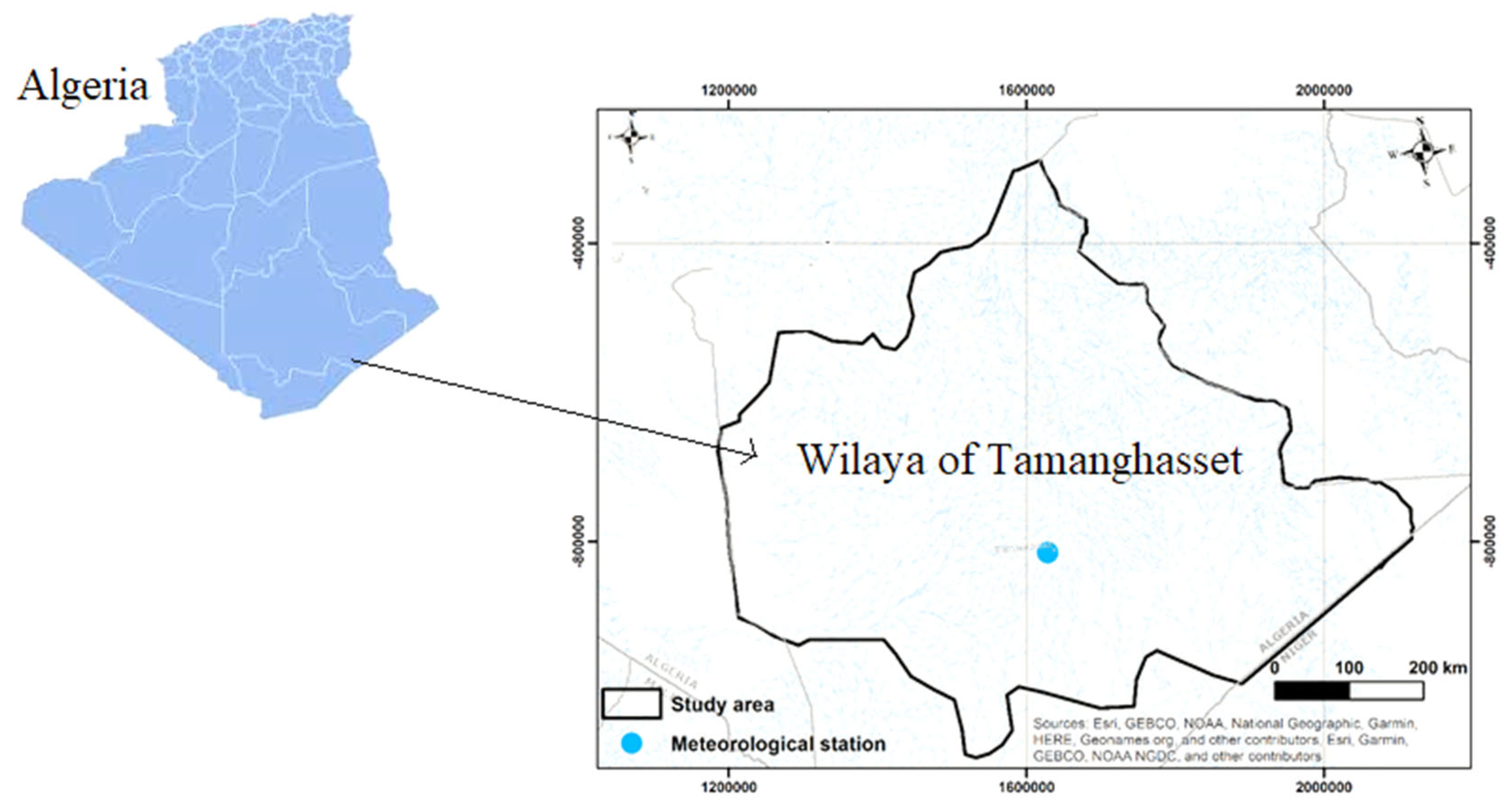
2.1. Study Area

Tamanghasset is a wilaya located in the extreme south of Algeria, in the central part of the Sahara Desert. Covering an area of approximately 335,562.5 km², it has a population of around 146,474 inhabitants. The region is characterized by arid climatic conditions and sparse hydrological networks, making it particularly vulnerable to water scarcity. Meteorological data for this study were collected from the Tamanghasset meteorological station, located within the town of Tamanghasset at 22°49′ N latitude and 5°27′ E longitude, at an elevation of 1372 m above sea level (Figure 1).

2.2. Dataset

Precipitations

The dataset employed in this study consists of monthly precipitation records from 1953 to 2021, collected at the Tamanghasset meteorological station, which is located at the town’s airport. These data were obtained from the Regional Meteorological Office of Tamanghasset. The study area is characterized by pronounced interannual variability in its rainfall regime, reflecting the highly irregular nature of precipitation typical of arid environments. The long-term average annual precipitation recorded at the Tamanghasset station is approximately 45.2 mm, although significant deviations from this mean have been observed during particularly wet years. August typically marks the peak of the rainy season, with the majority of precipitation concentrated between June and September, reaching an average of 7.7 mm during this period. In contrast, the precipitation levels during winter months are markedly lower, highlighting a strong seasonal disparity.

2.3. Classical Forecasting Methods

2.3.1. Autoregressive Integrated Moving Average (ARIMA)

The autoregressive integrated moving average (ARIMA) model remains one of the most widely applied techniques for analyzing non-stationary time series data. Unlike traditional regression models, ARIMA captures the dynamic structure of a time series by modeling its current values as a function of past (lagged) observations and stochastic error terms. ARIMA models combine three key components: auto regression (AR), integration (I) referring to the differencing required to achieve stationarity and moving average (MA). The standard notation ARIMA (_p, ^d, _q) specifies the order of each component, where _p denotes the number of autoregressive terms, ^d represents the degree of differencing required to attain stationarity, and _q indicates the number of lagged forecast errors in the prediction equation. The general form of the ARIMA (_p, ^d, _q) model can be expressed as described by Judge et al. (1988) [37].

$${∆}^d{y}_t=\delta +{\theta }_1{∆}^d{y}_{t-1}+{\theta }_2{∆}^d{y}_{t-2}+\dots +{\theta }_p{∆}^d{y}_{t-p}+e_{t-1}a{e}_{t-1}-a_2{e}_{t-2}{a}_q{e}_{t-2}$$

(1)

where ${∆}^d$ denotes differencing of order ^d, i.e., ${∆y}_t=y_t-y_{t-1}, {∆}^2{y}_t={∆y}_t-{∆y}_{t-1}$ and so forth, $y_{t-1},\dots ,y_{t-p}$ are past observations (lags), and $\delta , {\theta }_1,\dots , {\theta }_p$ are parameters (constant and coefficient) to be estimated similar to regression coefficients of the autoregressive process (AR) of order “_p” denoted by AR (_p) and is written as follows:

$$Y=\delta +{\theta }_1{y}_{t-1}+{\theta }_2{y}_{t-2}+\dots +{\theta }_p{y}_{t-p}+{\mathrm{e}}_{\mathrm{t}}$$

(2)

where $e_t$ is the forecast error, assumed to be independently distributed across time with mean $\theta$ and variance ${\theta }_{2}e, e_{t-1}, e_{t-2},\dots , e_{t-q}$ are past forecast errors, and $a_1, \dots , a_q$ are moving average (MA) coefficients. The MA model of order _q (i.e.,) MA (_q) can be written as

$$Y_t=e_t-a_1{a}_{t-1}-a_2{e}_{t-2}-\dots -a_q{e}_{t-q}$$

(3)

According to [38], the seasonal ARIMA model is denoted as ARIMA (_p, ^d, _q) (P, D, Q), where P represents the number of seasonal autoregressive terms, D indicates the number of seasonal differences required to achieve stationarity, and Q corresponds to the number of seasonal moving average terms. The development of an ARIMA model follows a structured approach proposed by Box and Jenkins, which involves three main stages: (a) model identification, (b) parameter estimation, and (c) diagnostic checking to validate the model’s adequacy.

2.3.2. ETS: Trend Component (T), a Seasonal Component (S), and an Error Term (E)

The error, trend, and seasonal (ETS) method is a widely used univariate time series forecasting approach that explicitly models error, trend, and seasonal components [39]. The strength of the ETS framework lies in its flexibility to capture a wide range of trend and seasonal patterns across different types of time series. According to [40], the ETS is composed of the following key components (

Table 1. Components.

	Seasonal Component
	N (None)	A (Additive)	M (Multiplicative)
N (None)	N (None)	Na	NM
A (Additive)	AN	AA	AM
Ad (Additive Damped)	AdN	AdA	AdM
M (Multiplicative)	MN	MA	MM

and

Table 2. ETS [30].

Model	Model	Model
ETS (M, M, N)	ETS (A, M, A)	ETS (M, N, M)
ETS (M, A, N)	ETS (A, Md, N)	ETS (M, N, A)
ETS (M, A, M)	ETS (A, Md, M)	ETS (M, N, N)
ETS (A, M, N)	ETS (A, N, A)	ETS (M, A, A)
ETS (A, N, N)	ETS (M, Ad, M)	ETS (A, Ad, M)
ETS (A, A, M)	ETS (M, Ad, N)	ETS (M, M, A)
ETS (M, M, M)	ETS (M, Md, M)	ETS (A, A, A)
ETS (A, N, M)	ETS (A, Ad, N)	ETS (A, Ad, A)
ETS (A, A, N)	ETS (M, Md, A)	ETS (M, Ad, A)

):

The ETS framework generates 30 distinct models, comprising 15 with additive errors and 15 with multiplicative errors, based on different combinations of trend and seasonal components. Not all models necessarily satisfy the underlying assumptions of the time series data; therefore, model selection becomes a critical step. Several model selection criteria, such as the Bayesian Information Criterion (BIC) and the corrected Akaike Information Criterion (AICc), can be employed to determine the most appropriate model among the candidate ETS specifications [40]. The Akaike Information Criterion (AIC) is calculated using the following formula:

$$AIC=-2\left({\displaystyle \frac{LL}{T}}\right)+{\displaystyle \frac{{2t}_p}{T}}$$

(4)

Which involves the AIC = Akaike Information Criterion, $LL$ = Log Likelihood, $t_p$ = Total Parameters, and T = the number of observations.

Akaike’s Information Criterion correction (AICc) can be calculated using the following equation:

$${AIC}_c=AIC+{\displaystyle \frac{2k(k+1)}{n-k-1}}$$

(5)

With ${\displaystyle \frac{2k(k+1)}{n-k-1}}$ as bias correction.

The Bayesian Information Criterion (BIC) can be calculated using the following equation:

$$BIC=-2LL+k\mathrm{l}\mathrm{n}\left(n\right)$$

(6)

where $LL$ = Log Likelihood, $k$ = Estimation of parameter model, and n = number of observations.

2.3.3. STL Decomposition Followed by the ETS Forecasting Model

The Seasonal-Trend decomposition using the Loess (STL) model is a robust technique for decomposing time series into interpretable components. STL separates a time series Y_t into three distinct elements: a seasonal component (St), a trend-cycle component (Tt), and a remainder or irregular component (R_t). Depending on the nature of the data, the decomposition can be either additive [39] or multiplicative [40]. After removing the seasonal component, the resulting seasonally adjusted series allows for improved modeling and forecasting of the underlying trend and irregular variations.

$$Y_t=S_t+T_t+R_t$$

(7)

$$Y_t=S_t\times T_{t }\times R_t$$

(8)

2.3.4. Neural Network Autoregressive (NNAR) Model

One important variant of artificial neural networks (ANNs) for time series forecasting is the neural network autoregressive (NNAR) model [41]. In the NNAR approach, lagged values of the time series are used as input predictors to forecast future observations. Unlike ARIMA models, NNAR models do not impose restrictions on parameters to ensure stationarity, offering greater flexibility in modeling complex, nonlinear dynamics [42]. Feed-forward neural networks are the most widely adopted architecture for time series modeling and forecasting.

The NNAR model is structured as a three-layer feed-forward network, comprising a linear combination function followed by a nonlinear activation function. The relationship between the model output y_t and the input lagged values (y_t – 1, …, y_t − p) can be mathematically expressed as follows:

$$y_t=w_0+\sum _{j=1}^h{w}_j.g\left(w_{0,j}+\sum _{j=1}^n{w}_{i,j}·y_{t-1}\right)+{\epsilon }_t$$

(9)

where $w_{i,j}$(i = 0, 1, 2, ..., n, j = 1, 2, ..., h) and $w_j$(j = 0, 1, 2, ..., h) are model parameters or connection weights; n is the number of input nodes; and h is the number of hidden nodes. A sigmoid function was used as the hidden layer transfer function shown in Equation (10). A linear function is the output layer’s most widely used activation function.

$$Sig\left(x\right)={\displaystyle \frac{1}{1+exp(-x)}}$$

(10)

Artificial neural networks (ANNs) are inspired by the functioning of the biological brain and are designed to model the complex relationships between input signals and an output response. In this study, two neural network architectures are employed: multilayer perceptrons (MLP) and neural network autoregressive models (NNARs).

2.3.5. TBATS Model: A State Space Approach for Complex Seasonal Time Series Forecasting

In TBATS models, seasonal patterns are captured using trigonometric terms [43]. The Box–Cox transformation is applied to address heteroscedasticity, while ARMA errors are incorporated to model short-term autocorrelation and dynamics. Damping parameters, if necessary, are used to model decaying trends alongside seasonal components. Consequently, TBATS models exhibit several advantageous properties.

According [44], (i) they are capable of handling autocorrelation within the residuals, (ii) they can capture nonlinear patterns in the time series, and (iii) they perform effectively with highly complex seasonal structures, including combinations of daily, weekly, and annual periodicities. In this study, the “tbats” function from the “forecast” package in the R environment was employed to fit the TBATS models, following the methodology outlined by [45].

Model components including the ARMA (p, q) structure, damping parameter, number of Fourier terms, and optimal Box–Cox transformation parameter were selected based on minimizing the Akaike Information Criterion (AIC). According to [45], the general form of the TBATS model is expressed as follows:

$$y_t^{\left(w\right)}=l_{t-1}+\varnothing b_{t-1}+{\sum }_{i=1}^T{s}_{t-m_i}^{\left(i\right)}+d_t$$

(11)

where $y_i^{\left(w\right)}$ indicates the Box–Cox transformation parameter (ω) applied to the observation $y_t$ at time t, $l_t$ is the local level, ϕ is the damped trend, b is the long-run trend, T denotes the seasonal pattern, $s_t^{\left(i\right)}$ is the seasonal component, $m_i$ denotes the seasonal periods and $d_t$ indicates an ARMA (p, q) process for residuals.

2.3.6. Performance Evaluation Metrics

The primary evaluation metrics used to compare the predictive performances of both single and hybrid models were the Root Mean Square Error (RMSE), the Mean Absolute Error (MAE), and the Mean Absolute Percentage Error (MAPE).

The corresponding equations are presented below:

$$\mathrm{M}\mathrm{A}\mathrm{E}={\displaystyle \frac{1}{\mathrm{n}}}{\sum }_{\mathrm{i}=1}^{\mathrm{n}}\left|{\mathrm{y}}_{\mathrm{i}}-{\hat{\mathrm{y}}}_{\mathrm{i}}\right|$$

(12)

$$\mathrm{M}\mathrm{A}\mathrm{P}\mathrm{E}={\displaystyle \frac{1}{\mathrm{n}}}{\sum }_{\mathrm{i}=1}^{\mathrm{n}}{\displaystyle \frac{\left|{\mathrm{y}}_{\mathrm{i}}-{\hat{\mathrm{y}}}_{\mathrm{i}}\right|}{{\mathrm{y}}_{\mathrm{i}}}} \mathrm{\ast } 100\%$$

(13)

$$\mathrm{R}\mathrm{M}\mathrm{S}\mathrm{E}=\sqrt{{\displaystyle \frac{1}{\mathrm{n}}}{\sum }_{\mathrm{i}=1}^{\mathrm{n}}{\left({\mathrm{y}}_{\mathrm{i}}-{\hat{\mathrm{y}}}_{\mathrm{i}}\right)}^2}$$

(14)

In the following equations, n denotes the number of observations, ${\mathrm{y}}_{\mathrm{i}}$ represents the actual values, and ${\hat{\mathrm{y}}}_{\mathrm{i}}$ denotes the predicted values. Both the Root Mean Square Error (RMSE) and the Mean Absolute Error (MAE) are scale-dependent metrics, as they are calculated based on different types of errors. Specifically, RMSE is based on squared errors, while MAE relies on absolute errors. Minimizing MAE leads to median forecasts, whereas minimizing RMSE tends to produce mean forecasts, making MAE generally easier to interpret. Unlike RMSE and MAE, the Mean Absolute Percentage Error (MAPE) is scale-independent, as it is computed from percentage errors [46].

This unit-free nature allows MAPE to be widely used for evaluating forecast accuracy across different datasets. However, MAPE has some limitations. It can become undefined or infinite when actual values are close to or equal to zero, and it tends to penalize negative errors more heavily than positive ones, potentially leading to biased forecasts. Nevertheless, its ability to compare forecasting accuracy across both single and multiple time series without dependency on the measurement scale makes it a valuable evaluation metric.

3. Results

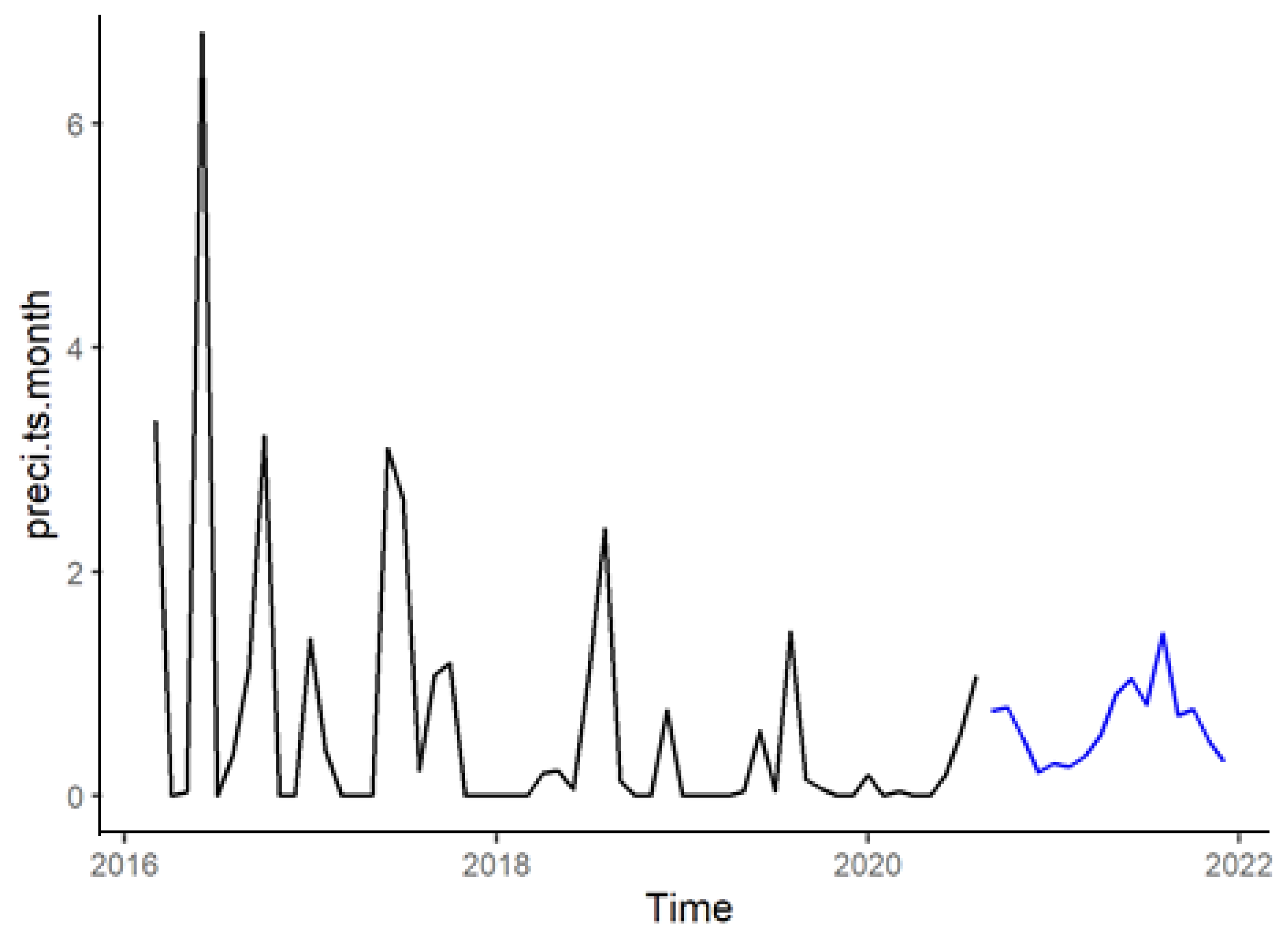
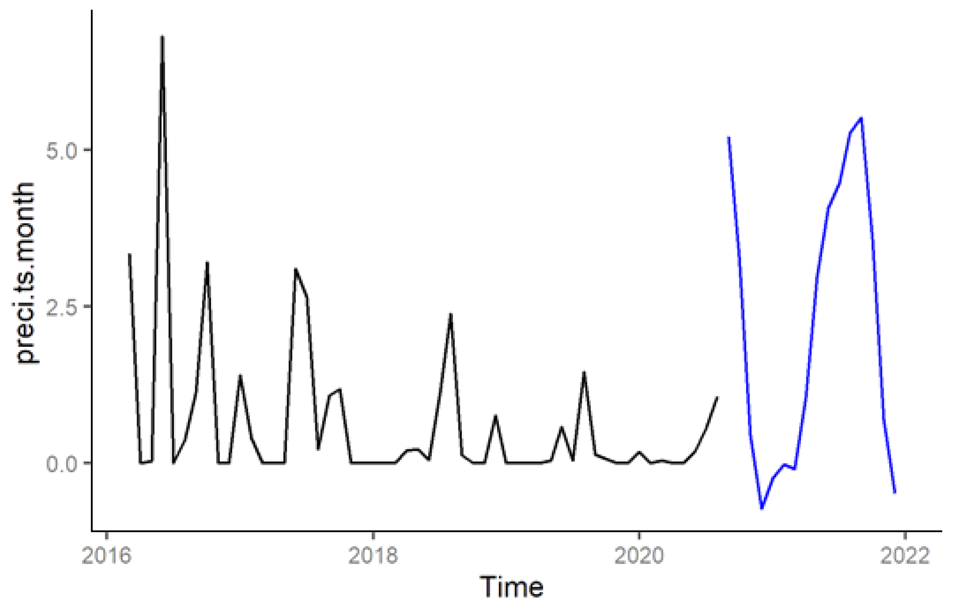
3.1. ARIMA Model for Statistical Forecasting of Monthly Precipitation

Statistical forecasting methods, such as the autoregressive integrated moving average (ARIMA) model, are widely used to identify potential relationships between predictor variables observed at time t and target variables forecasted at time (t + Δt). Their effectiveness has been confirmed by several recent studies [20,47,48,49,50,51]. ARIMA models offer an effective framework for improving predictive performance by capturing key temporal dynamics [52,53,54].

They integrate three fundamental components: autoregressive (AR) processes, integrated (I) differencing to achieve stationarity, and moving average (MA) processes to model the structure of residuals [43]. For the monthly precipitation series at the Tamanghasset station, the best-fitting model was identified as ARIMA (11, 1, 0) (6, 0, 0), selected based on the lowest standardized Bayesian Information Criterion (BIC) value of 1.076. The observed and forecasted precipitation values using this model are presented in (Figure 2).

3.2. ETS for Forecasting Monthly Precipitation at Tamanghasset Station

The ETS (Error, Trend, and Seasonality) model is a univariate time series forecasting method that explicitly focuses on modeling trend and seasonal components. Its effectiveness has been demonstrated in several recent studies, including [47,48,49]. In this study, monthly precipitation data from September 1953 to August 2020 at the Tamanghasset station were analyzed. Based on the minimum values of the Akaike Information Criterion (AIC), corrected Akaike Information Criterion (AICc), and Bayesian Information Criterion (BIC), the ETS (A, N, A) model representing additive error, no trend, and additive seasonality was selected as the most appropriate model for forecasting (Figure 3). According to the evaluation metrics, the ETS (A, N, A) model achieved an AIC of 7204, an AICc of 7204, and a BIC of 7274, demonstrating its superior predictive accuracy for monthly precipitation [39].

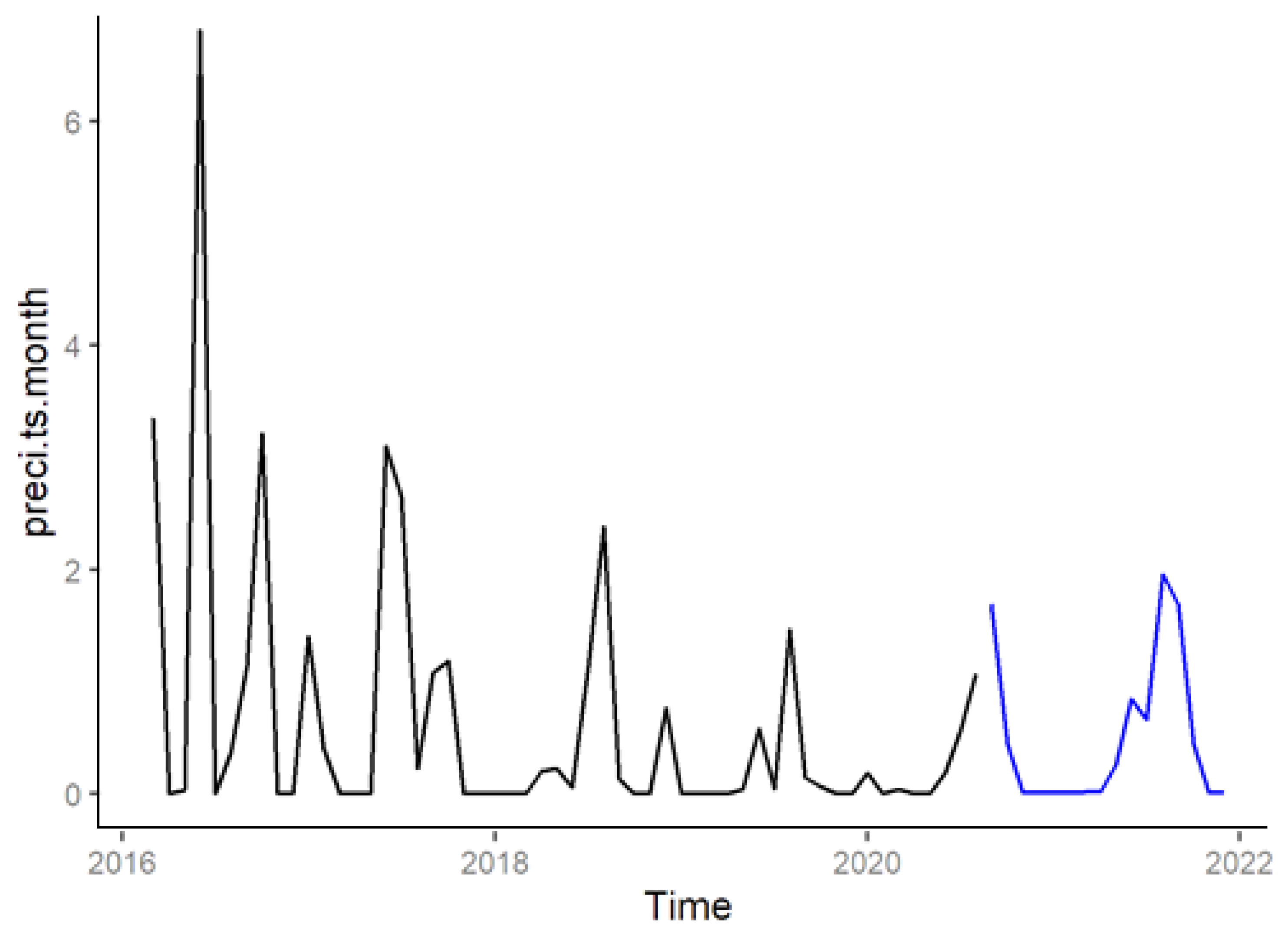
3.3. STL Decomposition of Monthly Precipitation at Tamanghasset Station

The STL (Seasonal-Trend decomposition using Loess) method is an algorithm designed to decompose a time series into the interpretable components trend, seasonality, and remainder through successive smoothing operations based on localized regression models [55]. First introduced in the Journal of Official Statistics, it relies on the application of the LOESS (Locally Estimated Scatterplot Smoothing) technique. The effectiveness of this method has been demonstrated in several recent studies, notably [56,57,58]. In this study, the STL method was applied to the monthly precipitation series from the Tamanghasset station (Figure 4). The decomposition revealed distinct seasonal patterns, while the remainder component exhibited several noticeable outliers (spikes), indicating the presence of irregular and extreme precipitation events.

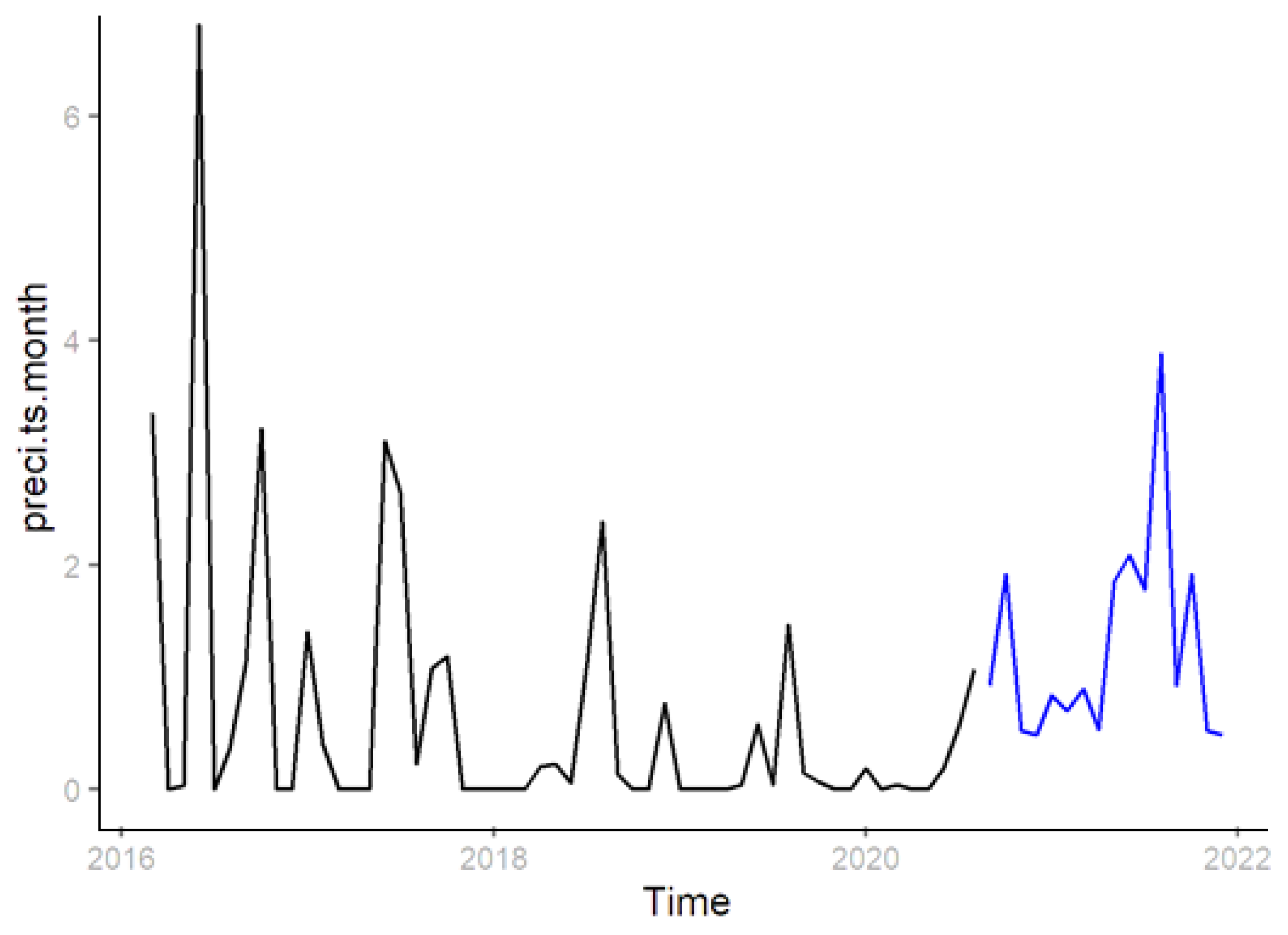
3.4. Forecasting Monthly Precipitation Using the NNAR Model

This approach made it possible to identify the most suitable forecasting model for the Tamanrasset station over the study period. Initial forecasts were produced using the STL-ETS (A, N, N) model, whose effectiveness has also been confirmed by several recent studies, including those by [59,60,61]. However, due to its superior predictive performance, the NNAR model was ultimately employed to forecast monthly precipitation volumes. In the first step, the NNAR model was fitted to the complete time series (1953–2020) for each district included in the analysis. The fitted models closely resembled those trained on the dataset, with the best-performing architecture identified as NNAR (25, 6, 12) (Figure 5). The NNAR (25, 6, 12) configuration was selected based on iterative testing and performance optimization using the Akaike Information Criterion (AIC) and residual diagnostics. The lag order of 25 reflects the extended memory effect in the precipitation series, while 12 accounts for annual seasonality. The choice of six hidden nodes ensures a balance between complexity and generalization capacity. Moreover, the observed precipitation patterns exhibit notable interannual and seasonal variability, which may be partially linked to large-scale atmospheric drivers such as the El Niño–Southern Oscillation (ENSO) or the North Atlantic Oscillation (NAO). Although not explicitly modeled in this study, these teleconnections offer a valuable avenue for future research to enhance the interpretability and climatic relevance of predictive models in arid regions.

The use of nonlinear models such as NNAR or TBATS is also theoretically supported by interdisciplinary research in environmental physics. For example, [62] demonstrated, through neutron scattering techniques, the presence of complex temporal dynamics in water-based systems, providing valuable insights into the nonlinear behaviors observed in precipitation time series. Citing such work reinforces the rationale for employing neural models in hydrological forecasting within arid environments.

These findings are consistent with recent research demonstrating the effectiveness of hybrid and wavelet-enhanced neural network models. For instance, wavelet-NNAR and SARIMA-NN models have shown promising results in hydrological time series forecasting in South Asian and North African contexts [59,60]. Such studies offer valuable methodological parallels and reinforce the relevance of hybrid or neural-based approaches in arid and semi-arid regions.

Before developing time series forecasting models, it was necessary to decompose the dataset to examine the irregular, trend, and seasonal behaviors of each series [62].

For this purpose, the TBATS model was employed due to its distinctive ability to capture complex patterns and multiple seasonalities within time series data. A key feature of TBATS is its use of trigonometric seasonal representations, which effectively extract intricate seasonal components during the decomposition process.

To model and estimate the contribution of each time series component, the dataset was divided into training (80%) and testing (20%) subsets, following the approach proposed by [62].

For the monthly precipitation data at Tamanghasset station, the TBATS (1, {0,0}, 0.93, {<12,3>}) model was identified as the most appropriate (Figure 6). This model achieved the best predictive performance, as indicated by the lowest Root Mean Square Error (RMSE = 8.713), Mean Absolute Error (MAE = 4.707), and Mean Absolute Percentage Error (MAPE = 144.6).

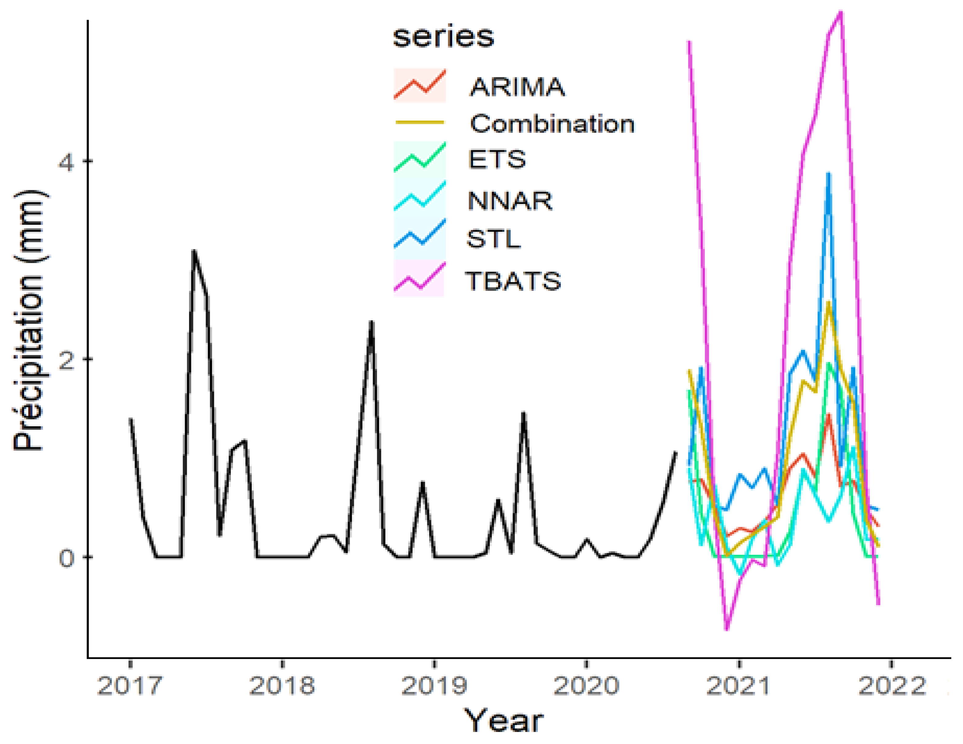
3.5. Selection of the Optimal Models Based on RMSE and MAPE Metrics

A detailed examination of the forecast accuracy metrics presented in

Table 3. Forecast accuracy for classical methods.

	ME	RMSE	MAE	MPE	MAPE	ACF1
ARIMA	0.1177	8.854	4.975	−3.586	149.4	−0.03284
ETS	−3.275	9.512	3.616	−23,572	23,680	0.02456
STL-ETS	0.1806	8.004	4.524	−1.418	146.7	0.0176
NNAR	0.005227	2.248	1.187	58.77	87.68	−0.0007443
TBATS	−0.2178	8.713	4.707	2.863	144.6	−0.03078

reveals significant differences in performance among the models tested. The NNAR (25, 6, 12) model demonstrates clear superiority across all key indicators, particularly RMSE (2.25) and MAE (1.19), highlighting its capacity to capture the nonlinear and seasonal structures of rainfall time series in hyper-arid regions such as Tamanghasset. Its very low residual autocorrelation (ACF1 = −0.0007) further indicates that the model has successfully extracted most of the temporal signal embedded in the data, with minimal information left in the residuals.

In contrast, classical linear models such as ARIMA and exponential smoothing techniques (ETS, STL-ETS) yield substantially higher error values. Notably, the ETS shows extremely high values of MAPE (23,680) and MPE (−23,572), which are attributable to its inability to handle months with very low or zero precipitation—a common feature of arid environments. These outliers skew percentage-based metrics, revealing the limitations of additive models in such settings.

The TBATS model performs moderately well, showing improved handling of seasonal components compared to ETS but still lagging behind NNAR. This suggests that while TBATS is well suited for complex seasonality, it may struggle with nonlinearity or extreme values inherent in desert climatology. Moreover, the residual autocorrelations for ARIMA and TBATS (−0.03) imply that some predictable patterns remain unmodeled.

Overall, the superiority of the NNAR model can be attributed to its capacity to learn flexible nonlinear relationships and to adapt to irregular seasonal structures without requiring prior decomposition. This aligns with previous findings in arid and semi-arid forecasting studies (e.g., [4,6]). These results confirm that data-driven models, particularly neural networks enhanced with appropriate lag selection, are well suited for precipitation prediction in hydrologically challenging environments.

Future work should consider uncertainty quantification, such as confidence intervals around RMSE and MAPE, to further assess the robustness of the model comparisons. Additionally, ensemble approaches combining NNAR with other learning algorithms (e.g., hybrid wavelet-NNAR or SARIMA-NN) may enhance generalizability and interpretability, particularly under changing climate conditions (Figure 7).

4. Conclusions

This study focused on modeling monthly precipitation in the Tamanghasset region using various machine learning approaches. A comparative analysis was conducted to assess the performance of each model in fitting the observed data. Among the models evaluated, the neural network autoregressive (NNAR) model demonstrated superior performance across all series based on the training dataset. Furthermore, NNAR exhibited the highest predictive accuracy, as reflected by the coefficient of determination (R²), indicating its effectiveness in explaining the variability of the time series through error minimization. In the current context, the application of advanced machine learning techniques proves valuable for modeling climatic variables. This study contributes to the growing body of research on the predictive modeling of climate factors, providing insights that may support the decision-making of researchers and policymakers. Therefore, systematically evaluating and comparing the forecasting capabilities of machine learning models is important for selecting the most appropriate model for predicting future observations. The findings also suggest a potential decline in precipitation levels in the coming years, emphasizing the need for proactive measures to address water resource challenges, particularly in arid and hyper-arid regions such as Tamanghasset.

References

1. Watson, F.; Austin, P. Physiology of human fluid balance. Anaesth. Intensiv. Care Med. 2021, 22, 644–651. [Google Scholar] [CrossRef]
2. Ma, R.; Han, J.; Alrowais, R.; Zhou, J.; Li, R. Atmospheric water as alternative and universal resources: From the energy perspective. Nano Energy 2025, 140, 111012. [Google Scholar] [CrossRef]
3. Jahan Rakib, M.R.; Mohiuddin, M.; Al Masud, M.A.; Murshed, M.F.; Senapathi, V.; Islam, M.A.; Jakariya, M. Exploring the impact of microplastics in groundwater on human health: A comprehensive review. Curr. Opin. Environ. Sci. Health 2025, 44, 100605. [Google Scholar] [CrossRef]
4. Ahmed, A.A.; Sayed, S.; Abdoulhalik, A.; Moutari, S.; Oyedele, L. Applications of machine learning to water resources management: A review of present status and future opportunities. J. Clean. Prod. 2024, 441, 140715. [Google Scholar] [CrossRef]
5. Chahid, M.; Stitou El Messari, J.E.; Hilal, I.; Aqnouy, M. Application of the DRASTIC-LU/LC method combined with machine learning models to assess and predict the vulnerability of the Rmel aquifer (Northwest, Morocco). Groundw. Sustain. Dev. 2024, 27, 101345. [Google Scholar] [CrossRef]
6. Latif, S.D.; Mohammed, D.O.; Jaafar, A. Developing an innovative machine learning model for rainfall prediction in a semi-arid region. J. Hydroinform. 2024, 26, 904–914. [Google Scholar] [CrossRef]
7. Ahmadov, E. Water resources management to achieve sustainable development in Azerbaijan. Sustain. Futures 2020, 2, 100030. [Google Scholar] [CrossRef]
8. En-nagre, K.; Aqnouy, M.; Bouadila, A.; Et-Takaouym, C.; Chahid, M.; Bouizrou, I.; Hilal, I.; Stitou El Messari, J.E.; Tariq, A. Assessment of Three Satellite Precipitation Products for Hydrological Studies in a Data-Scarce Context: Ouarzazate Basin, Southern Morocco. Nat. Hazards Res. 2025, in press. [CrossRef]
9. Et-Takaouy, C.; Aqnouy, M.; Boukholla, A.; Stitou El Messari, J.E. Exploring the spatio-temporal variability of four satellite-based precipitation products (SPPs) in northern Morocco: A comparative study of complex climatic and topographic conditions. Mediterr. Geosci. Rev. 2024, 6, 123–144. [Google Scholar] [CrossRef]
10. Akram, M.; Hamid, A. A comprehensive review on water balance. Biomed. Prev. Nutr. 2013, 3, 193–195. [Google Scholar] [CrossRef]
11. Aqnouy, M.; Ommane, Y.; Ouallali, A.; Gourfi, A.; Ayele, G.T.; El Yousfi, Y.; Bouizrou, I.; Stitou El Messari, J.E.; Zettam, A.; Melesse, A.M.; et al. Evaluation of TRMM 3B43 V7 precipitation data in varied Moroccan climatic and topographic zones. Mediterr. Geosci. Rev. 2024, 6, 159–175. [Google Scholar] [CrossRef]
12. Yang, T.-H.; Liu, W.-C. A general overview of the risk-reduction strategies for floods and droughts. Sustainability 2020, 12, 2687. [Google Scholar] [CrossRef]
13. Morante-Carballo, F.; Montalván-Burbano, N.; Quiñonez-Barzola, X.; Jaya-Montalvo, M.; Carrión-Mero, P. What Do We Know about Water Scarcity in Semi-Arid Zones? A Global Analysis and Research Trends. Water 2022, 14, 2685. [Google Scholar] [CrossRef]
14. Wang, M.; Chen, Y.; Li, J.; Zhao, Y. Spatiotemporal evolution and driving force analysis of drought characteristics in the Yellow River Basin. Ecol. Indic. 2025, 170, 113007. [Google Scholar] [CrossRef]
15. Zaerpour, M.; Hatami, S.; Ballarin, A.S.; Knoben, W.J.M.; Papalexiou, S.M.; Pietroniro, A.; Clark, M.P. Impacts of agriculture and snow dynamics on catchment water balance in the U.S. and Great Britain. Commun. Earth Environ. 2024, 5, 733. [Google Scholar] [CrossRef] [PubMed]
16. Bista, S.; Baniya, R.; Sharma, S.; Ghimire, G.R.; Panthi, J.; Prajapati, R.; Thapa, B.R.; Talchabhadel, R. Hydrologic applicability of satellite-based precipitation estimates for irrigation water management in the data-scarce region. J. Hydrol. 2024, 636, 131310. [Google Scholar] [CrossRef]
17. Bouizrou, I.; Bouadila, A.; Aqnouy, M.; Gourfi, A. Assessment of remotely sensed precipitation products for climatic and hydrological studies in arid to semi-arid data-scarce region, central-western Morocco. Remote Sens. Appl. Soc. Environ. 2023, 30, 100976. [Google Scholar] [CrossRef]
18. Deng, Y.; Wang, X.; Ruan, H.; Lin, J.; Chen, X.; Chen, Y.; Duan, W.; Deng, H. The magnitude and frequency of detected precipitation determine the accuracy performance of precipitation data sets in the high mountains of Asia. Sci. Rep. 2024, 14, 17251. [Google Scholar] [CrossRef] [PubMed]
19. Sham, F.A.F.; El-Shafie, A.; Jaafar, W.Z.W.; S, A.; Sherif, M.; Ahmed, A.N. Advances in AI-based rainfall forecasting: A comprehensive review of past, present, and future directions with intelligent data fusion and climate change models. Results Eng. 2025, 27, 105774. [Google Scholar] [CrossRef]
20. Alsumaiei, A.A. Long-term rainfall forecasting in arid climates using artificial intelligence and statistical recurrent models. J. Eng. Res. 2024, 13, 1594–1602. [Google Scholar] [CrossRef]
21. Higuera Roa, O.; Cotti, D.; Aste, N.; Bustillos-Ardaya, A.; Schneiderbauer, S.; Tourino Soto, I.; Román-Dañobeytia, F.; Walz, Y. Deriving targeted intervention packages of nature-based solutions for climate change adaptation and disaster risk reduction: A geospatial multi-criteria approach for building resilience in the Puna region, Peru. Nat.-Based Solut. 2023, 4, 100090. [Google Scholar] [CrossRef]
22. He, R.; Zhang, L.; Chew, A.W.Z. Modeling and predicting rainfall time series using seasonal-trend decomposition and machine learning. Knowl.-Based Syst. 2022, 251, 109125. [Google Scholar] [CrossRef]
23. Ayiah-Mensah, F.; Bosson-Amedenu, S.; Baah, E.M.; Addor, J.A. Advancements in seasonal rainfall forecasting: A seasonal auto-regressive integrated moving average model with outlier adjustments for Ghana’s Western Region. Sci. Afr. 2025, 28, e02632. [Google Scholar] [CrossRef]
24. Effrosynidis, D.; Spiliotis, E.; Sylaios, G.; Arampatzis, A. Time series and regression methods for univariate environmental forecasting: An empirical evaluation. Sci. Total Environ. 2023, 875, 162580. [Google Scholar] [CrossRef] [PubMed]
25. Madi, H.; Bedjaoui, A.; Elhoussaoui, A.; Elbakai, L.O.; Bounaama, A. Flood Vulnerability Mapping and Risk Assessment Using Hydraulic Modeling and GIS in Tamanrasset Valley Watershed, Algeria. J. Ecol. Eng. 2023, 24, 35–48. [Google Scholar] [CrossRef] [PubMed]
26. Monjo, R.; Meseguer-Ruiz, O. Review: Fractal Geometry in Precipitation. Atmosphere 2024, 15, 135. [Google Scholar] [CrossRef]
27. Chahid, M.; Hilal, I.; En-Nagre, K.; Et-Takaouy, C.; El Messari, J.E.S.; Aqnouy, M. Assessment and modeling of the hydrochemical evolution of the Rmel aquifer (NW Morocco): Geostatistical approaches and machine learning for sustainable management. Mediterr. Geosci. Rev. 2025, 7, 341–362. [Google Scholar] [CrossRef]
28. Chahid, M.; Hilal, I.; Et-Takaouy, C.; En-Nagre, K.; Stitou El Messari, J.E.; Mansour, M.R.A.; Aqnouy, M. Comparison of groundwater pollution vulnerability assessments via the DRASTIC-LU and DRASTIC-LU-NO3 methods in the Ouled Ogbane aquifer, Northwest Morocco. Environ. Sci. Pollut. Res. 2025, 32, 16261–16279. [Google Scholar] [CrossRef] [PubMed]
29. Hurtado, A.R.; Díaz-Cano, E.; Berbel, J. The paradox of success: Water resources closure in Axarquia (southern Spain). Sci. Total Environ. 2024, 946, 174318. [Google Scholar] [CrossRef] [PubMed]
30. Khacheba, R.; Cherfaoui, M.; Hartani, T.; Drouiche, N. The nexus approach to water–energy–food security: An option for adaptation to climate change in Algeria. Desalin. Water Treat. 2018, 131, 30–33. [Google Scholar] [CrossRef]
31. Gastineau, R.; Hamedi, C.; Baba Hamed, M.B.; Abi-Ayad, S.M.E.A.; Bąk, M.; Lemieux, C.; Turmel, M.; Dobosz, S.; Wróbel, R.J.; Kierzek, A.; et al. Morphological and molecular identification reveals that waters from an isolated oasis in Tamanrasset (extreme South of Algerian Sahara) are colonized by opportunistic and pollution-tolerant diatom species. Ecol. Indic. 2021, 121, 107104. [Google Scholar] [CrossRef]
32. Sahnoune, F.; Belhamel, M.; Zelmat, M.; Kerbachi, R. Climate change in Algeria: Vulnerability and strategy of mitigation and adaptation. Energy Procedia 2013, 36, 1286–1294. [Google Scholar] [CrossRef]
33. Hadj Arab, A.; Chenlo, F.; Benghanem, M. Loss-of-load probability of photovoltaic water pumping systems. Sol. Energy 2004, 76, 713–723. [Google Scholar] [CrossRef]
34. Chaulagain, S.; Lamichhane, M.; Chaulagain, U. A review of current trends, challenges, and future perspectives in machine learning applications to water resources in Nepal. J. Hazard. Mater. Adv. 2025, 18, 100678. [Google Scholar] [CrossRef]
35. Olawade, D.B.; Wada, O.Z.; Ige, A.O.; Egbewole, B.I.; Olojo, A.; Oladapo, B.I. Artificial intelligence in environmental monitoring: Advancements, challenges, and future directions. Hyg. Environ. Health Adv. 2024, 12, 100114. [Google Scholar] [CrossRef]
36. Bolan, S.; Padhye, L.P.; Jasemizad, T.; Govarthanan, M.; Karmegam, N.; Wijesekara, H.; Amarasiri, D.; Hou, D.; Zhou, P.; Biswal, B.K.; et al. Impacts of climate change on the fate of contaminants through extreme weather events. Sci. Total Environ. 2024, 909, 168388. [Google Scholar] [CrossRef] [PubMed]
37. Judge, G.G.; Hill, R.C.; Griffiths, W.E.; Lutkepohl, H.; Lee, T. Introduction to the Theory and Practice of Econometrics, 2nd ed.; John Wiley: New York, NY, USA, 1988; pp. xxxv + 1024. ISBN 0-471-62414-4. [Google Scholar]
38. Box, G.E.P.; Jenkins, G.M. Time Series Analysis, Forecasting and Control, Revised ed.; Holden-Day: San Francisco, CA, USA, 1994. [Google Scholar]
39. Jofipasi, C.A.; Miftahuddin, M.; Sofyan, H. Selection for the best ETS (error, trend, seasonal) model to forecast weather in the Aceh Besar District. IOP Conf. Ser. Mater. Sci. Eng. 2018, 352, 012055. [Google Scholar] [CrossRef]
40. Hyndman, R.J.; Khandakar, Y. Automatic time series forecasting: The forecast package for R. J. Stat. Softw. 2008, 27, 1–22. [Google Scholar] [CrossRef]
41. Tealab, A.; Hefny, H.; Badr, A. Forecasting of nonlinear time series using ANN. Future Comput. Inform. J. 2017, 2, 39–47. [Google Scholar] [CrossRef]
42. Thoplan, R. Random Forests for Poverty Classification. Int. J. Sci. Basic Appl. Res. 2014, 17, 252–259. [Google Scholar]
43. Perone, G. Comparison of ARIMA, ETS, NNAR, TBATS and hybrid models to forecast the second wave of COVID-19 hospitalizations in Italy. Eur. J. Health Econ. 2022, 23, 917–940. [Google Scholar] [CrossRef] [PubMed]
44. Talkhi, N.; Akhavan Fatemi, N.; Ataei, Z.; Jabbari Nooghabi, M. Modeling and forecasting number of confirmed and death caused COVID-19 in IRAN: A comparison of time series forecasting methods. Biomed. Signal Process. Control 2021, 66, 102494. [Google Scholar] [CrossRef] [PubMed]
45. de Livera, A.M.; Hyndman, R.J.; Snyder, R.D. Forecasting time series with complex seasonal patterns using exponential smoothing. J. Am. Stat. Assoc. 2011, 106, 1513–1527. [Google Scholar] [CrossRef]
46. Kim, S.; Kim, H. A new metric of absolute percentage error for intermittent demand forecasts. Int. J. Forecast. 2016, 32, 669–679. [Google Scholar] [CrossRef]
47. Arumugam, P.; Saranya, R. Outlier Detection and Missing Value in Seasonal ARIMA Model Using Rainfall Data. Mater. Today Proc. 2018, 5, 1791–1799. [Google Scholar] [CrossRef]
48. Bari, S.H.; Rahman, M.T.; Hussain, M.M.; Ray, S. Forecasting Monthly Precipitation in Sylhet City Using ARIMA Model. Civ. Environ. Res. 2015, 7, 69–77. [Google Scholar]
49. Dahiya, P.; Kumar, M.; Manhas, S.; Saini, A.; Yadav, S.K.; Sirohi, S.; Kamboj, M.; Khichar, M.L.; Mishra, E.P.; Sharma, V.; et al. Time series study of climate variables utilising a seasonal ARIMA technique for the Indian states of Punjab and Haryana. Discov. Appl. Sci. 2024, 6, 650. [Google Scholar] [CrossRef]
50. Abd-Elhamid, H.F.; El-Dakak, A.M.; Zeleňáková, M.; K, S.O.; Mahdy, M.; Abd El Ghany, S.H. Rainfall forecasting in arid regions in response to climate change using ARIMA and remote sensing. Geomat. Nat. Hazards Risk 2024, 15, 2347414. [Google Scholar] [CrossRef]
51. Parviz, L.; Ghorbanpour, M. Assimilation of PSO and SVR into an improved ARIMA model for monthly precipitation forecasting. Sci. Rep. 2024, 14, 12107. [Google Scholar] [CrossRef] [PubMed]
52. Kim, J.; Kim, H.; Kim, H.G.; Lee, D.; Yoon, S. A comprehensive survey of deep learning for time series forecasting: Architectural diversity and open challenges. Artif. Intell. Rev. 2025, 58, 216. [Google Scholar] [CrossRef]
53. Ray, S.S.; Verma, R.K.; Singh, A.; Myung, S.; Park, Y.I.; Kim, I.C.; Lee, H.K.; Kwon, Y.-N. Exploration of time series model for predictive evaluation of long-term performance of membrane distillation desalination. Process Saf. Environ. Prot. 2022, 160, 1–12. [Google Scholar] [CrossRef]
54. Sangeetha, S.K.B.; Mathivanan, S.K.; Rajadurai, H.; Cho, J.; Easwaramoorthy, S.V. A multi-modal geospatial–temporal LSTM based deep learning framework for predictive modeling of urban mobility patterns. Sci. Rep. 2024, 14, 31579. [Google Scholar]
55. Sanchez-Vazquez, M.J.; Nielen, M.; Gunn, G.J.; Lewis, F.I. Using seasonal-trend decomposition based on loess (STL) to explore temporal patterns of pneumonic lesions in finishing pigs slaughtered in England, 2005–2011. Prev. Vet. Med. 2012, 104, 65–73. [Google Scholar] [CrossRef] [PubMed]
56. Apaydin, H.; Taghi Sattari, M.; Falsafian, K.; Prasad, R. Artificial intelligence modelling integrated with Singular Spectral analysis and Seasonal-Trend decomposition using Loess approaches for streamflow predictions. J. Hydrol. 2021, 600, 126506. [Google Scholar] [CrossRef]
57. Lem, K.H. The STL-ARIMA approach for seasonal time series forecast: A preliminary study. ITM Web Conf. 2024, 67, 01008. [Google Scholar] [CrossRef]
58. Trull, O.; García-Díaz, J.C.; Peiró-Signes, A. Multiple seasonal STL decomposition with discrete-interval moving seasonalities. Appl. Math. Comput. 2022, 433, 127398. [Google Scholar] [CrossRef]
59. Khalek, M.A.; Ali, M.A. Comparative Study of Wavelet-SARIMA and Wavelet-NNAR Models for Groundwater Level in Rajshahi District. IOSR J. Environ. Sci. 2016, 10, 1–15. [Google Scholar]
60. Ahmar, A.S.; Singh, P.K.; Ruliana, R.; Pandey, A.K.; Gupta, S. Comparison of ARIMA, SutteARIMA, and Holt-Winters, and NNAR Models to Predict Food Grain in India. Forecasting 2023, 5, 138–152. [Google Scholar] [CrossRef]
61. Saranya, M.S.; Vinish, V.N. A comparative evaluation of streamflow prediction using the SWAT and NNAR models in the Meenachil River Basin of Central Kerala, India. Water Sci. Technol. 2023, 88, 2002–2018. [Google Scholar] [CrossRef] [PubMed]
62. Ray, M.; Sahoo, K.C.; Abotaleb, M.; Ray, S.; Sahu, P.K.; Mishra, P.; GhaziAlKhatib, A.; SankarDas, S.; Jain, V.; Balloo, R. Modeling and forecasting meteorological factors using BATS and TBATS models for the Keonjhar district of Orissa. Mausam 2022, 73, 555–564. [Google Scholar] [CrossRef]
Figure 1. Location of the study area in Tamanghasset, Algeria.
Geosciences 15 00273 g001
Figure 2. ARIMA model application for monthly precipitation forecasting (in blue: forcasted).
Geosciences 15 00273 g002
Figure 3. Forecasts the monthly rainfall with ETS (in blue: forcasted).
Geosciences 15 00273 g003
Figure 4. Forecasts the monthly rainfall with STL+ETS (in blue: forcasted).
Geosciences 15 00273 g004
Figure 5. Forecasts from the NNAR model for rainfall data series (in blue: forcasted).
Geosciences 15 00273 g005
Figure 6. Forecasts the monthly rainfall with TBATS (in blue: forcasted).
Geosciences 15 00273 g006
Figure 7. Forecast combinations.
Geosciences 15 00273 g007