
Advancing Scalable Methods for Surface Water Monitoring: A Novel Integration of Satellite Observations and Machine Learning Techniques


Abstract
1. Introduction
- High vertical accuracy lidar-derived DEMs from airborne and spaceborne systems to correct and refine existing topographic data.
- Synthetic Aperture Radar (SAR) imagery for water extent mapping, leveraging SAR’s ability to penetrate cloud cover and vegetation, providing all-weather water body detection.
- A robust volume estimation technique combining water extent and DEM data from multi-data fusion.
2. Materials and Methods
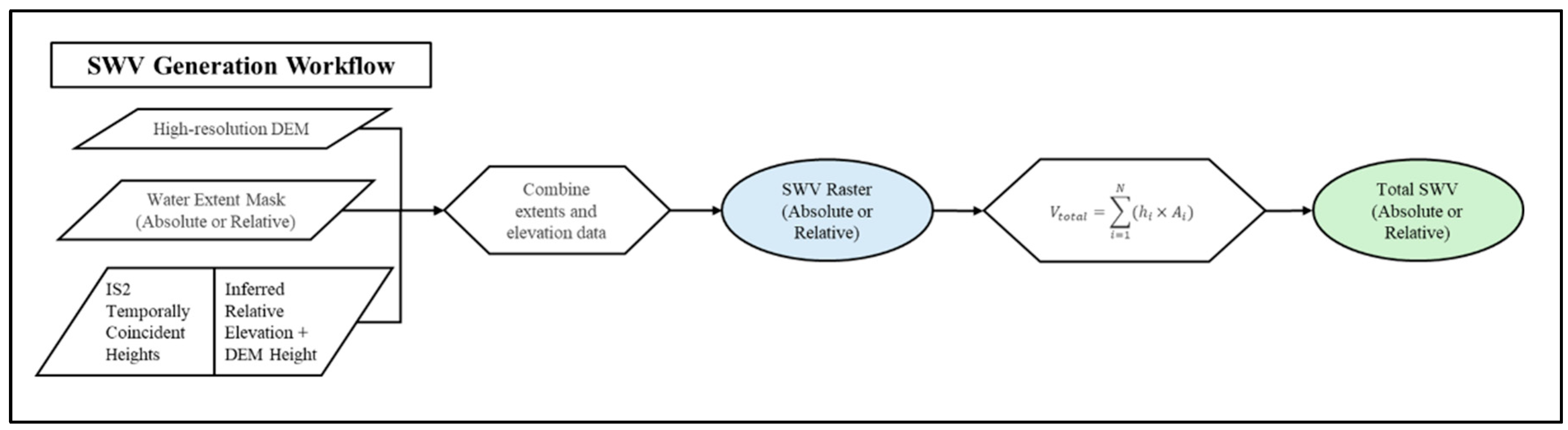
2.1. Volume Estimation Overview
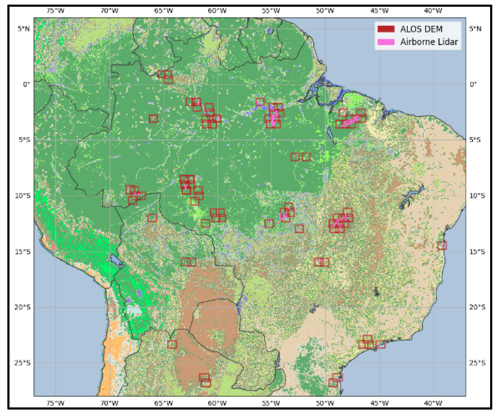
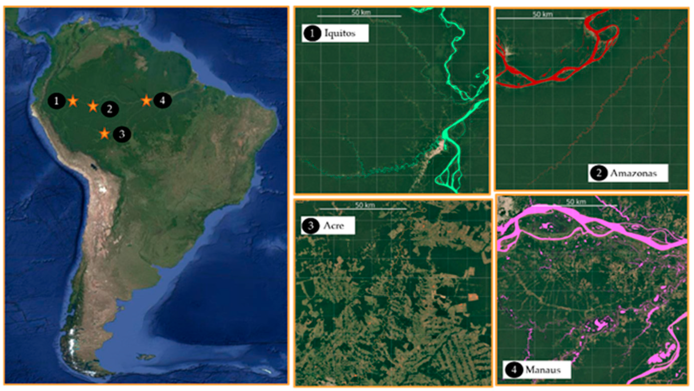
2.2. Study Region
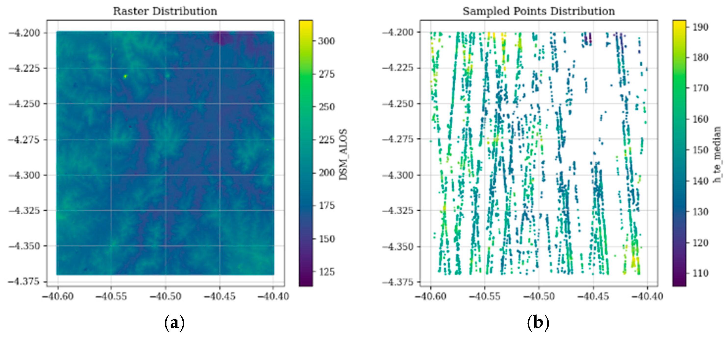
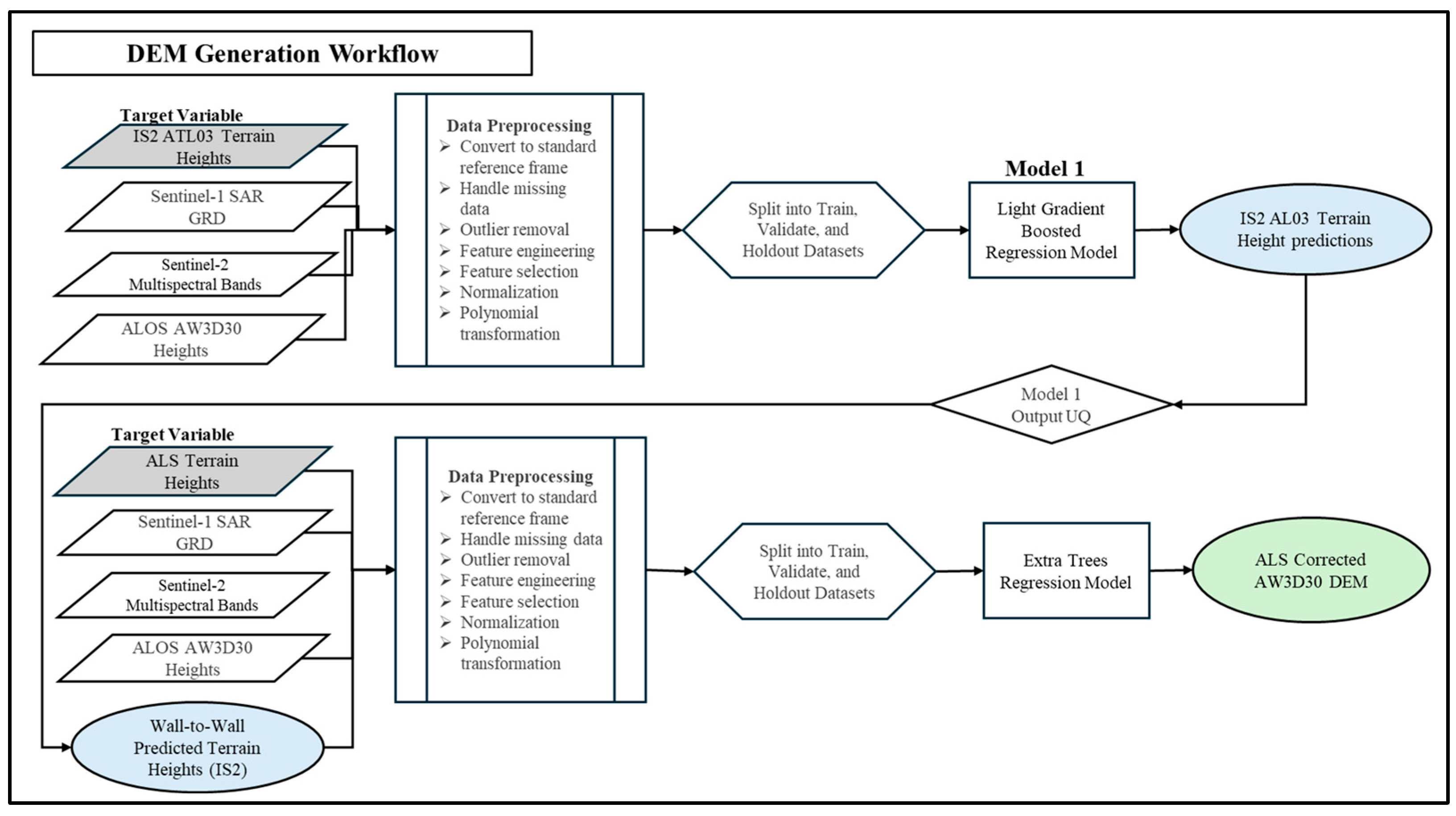
2.3. DEM Generation
2.3.1. Machine Learning Data Inputs
AW3D30 (Terrain Reference)
ICESat-2 (Terrain Reference)
Sentinel-1
Sentinel-2
Airborne Lidar Surveys (Terrain Reference)
2.3.2. Initial Assessment
2.3.3. Model Selection and Training
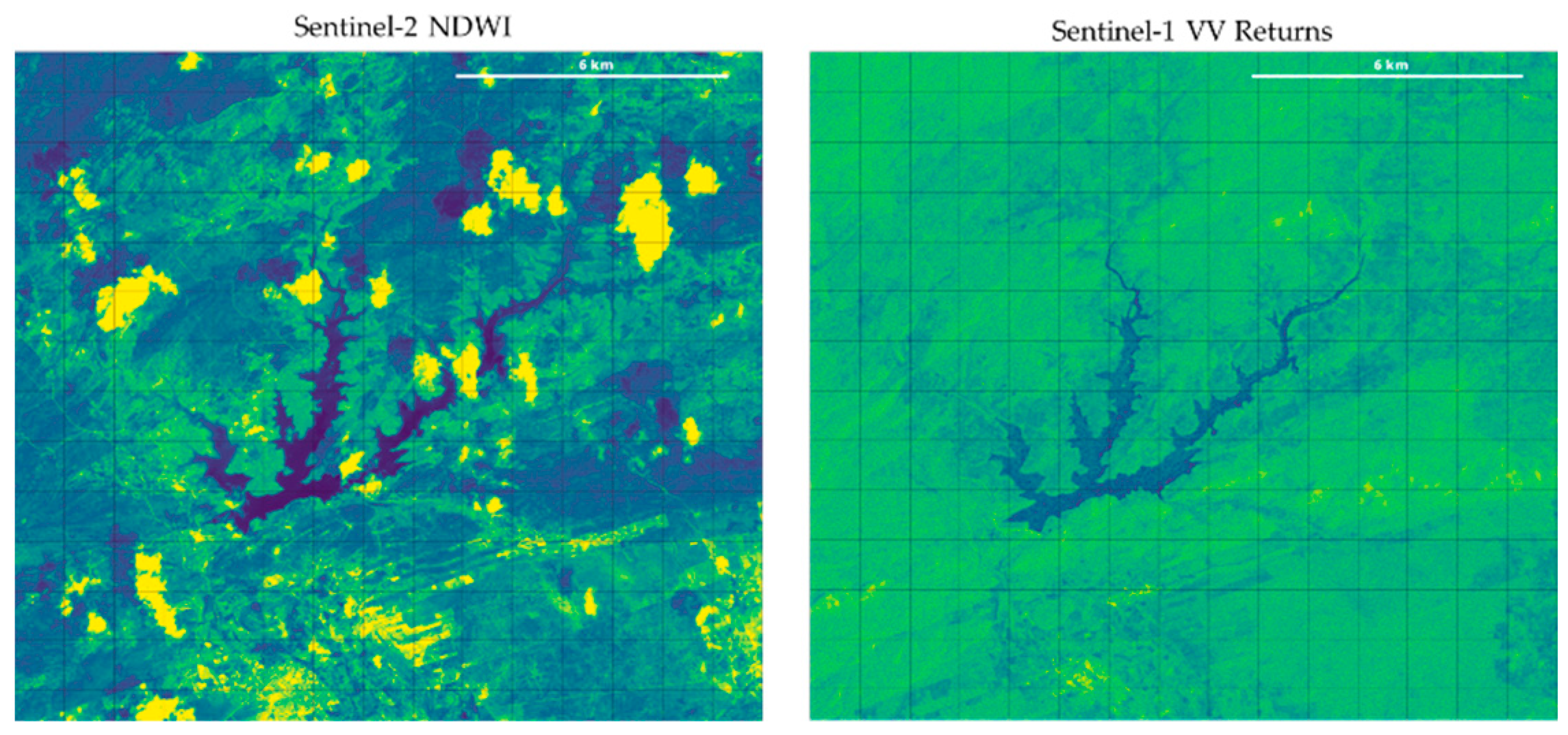
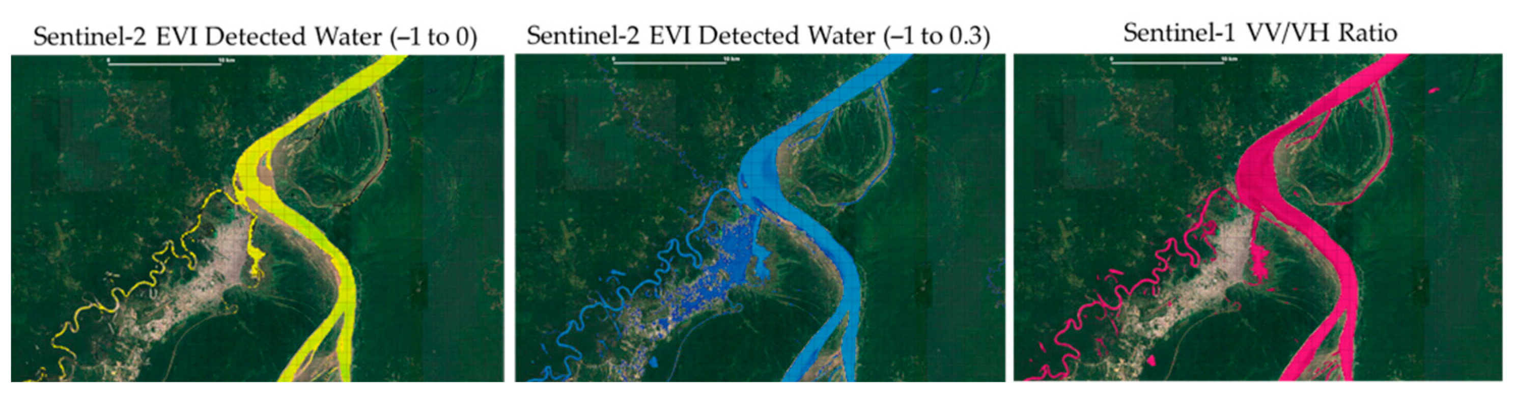
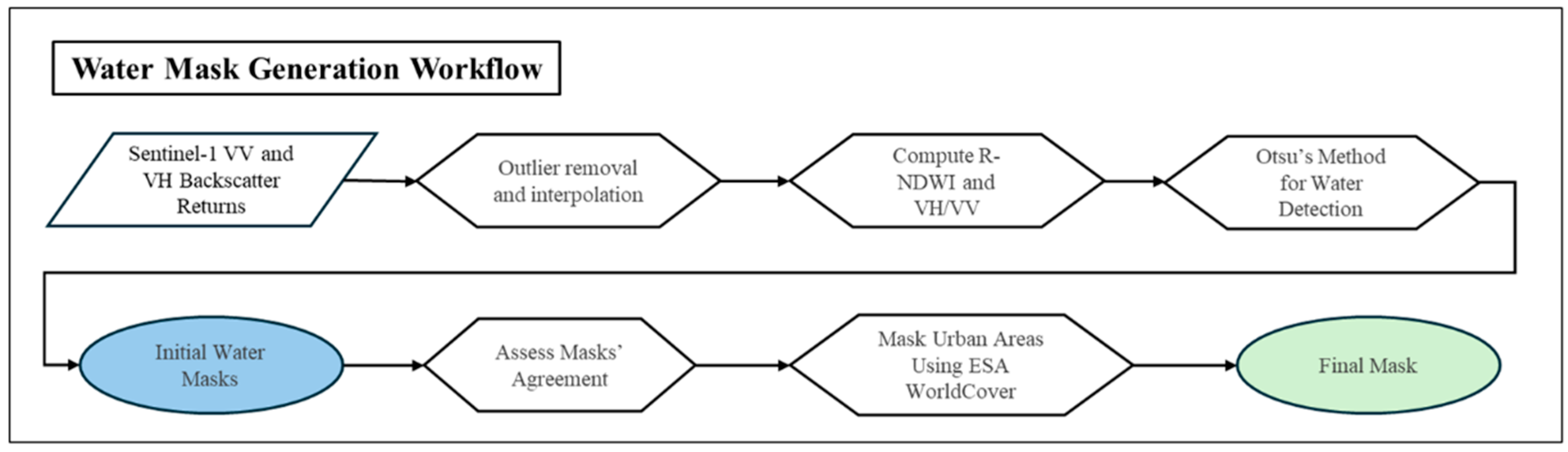
2.4. Surface Water Mapping in All-Weather Conditions
Thresholding Approach
3. Results
3.1. Validation Regions
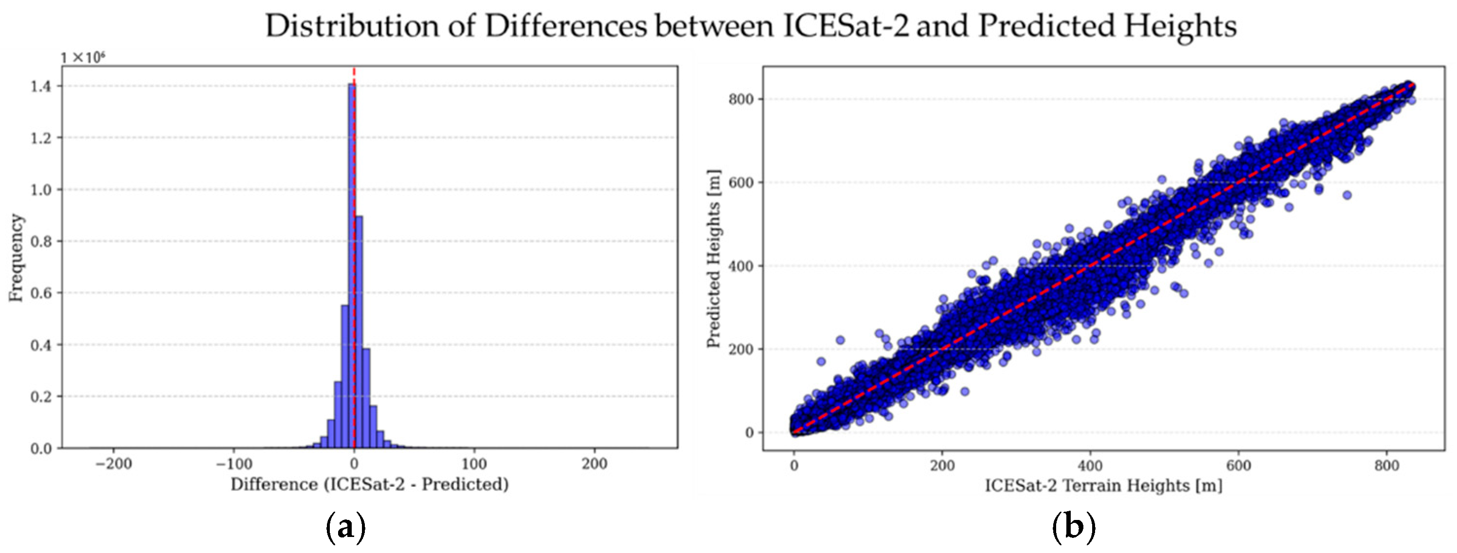
3.2. ML Model Assessment
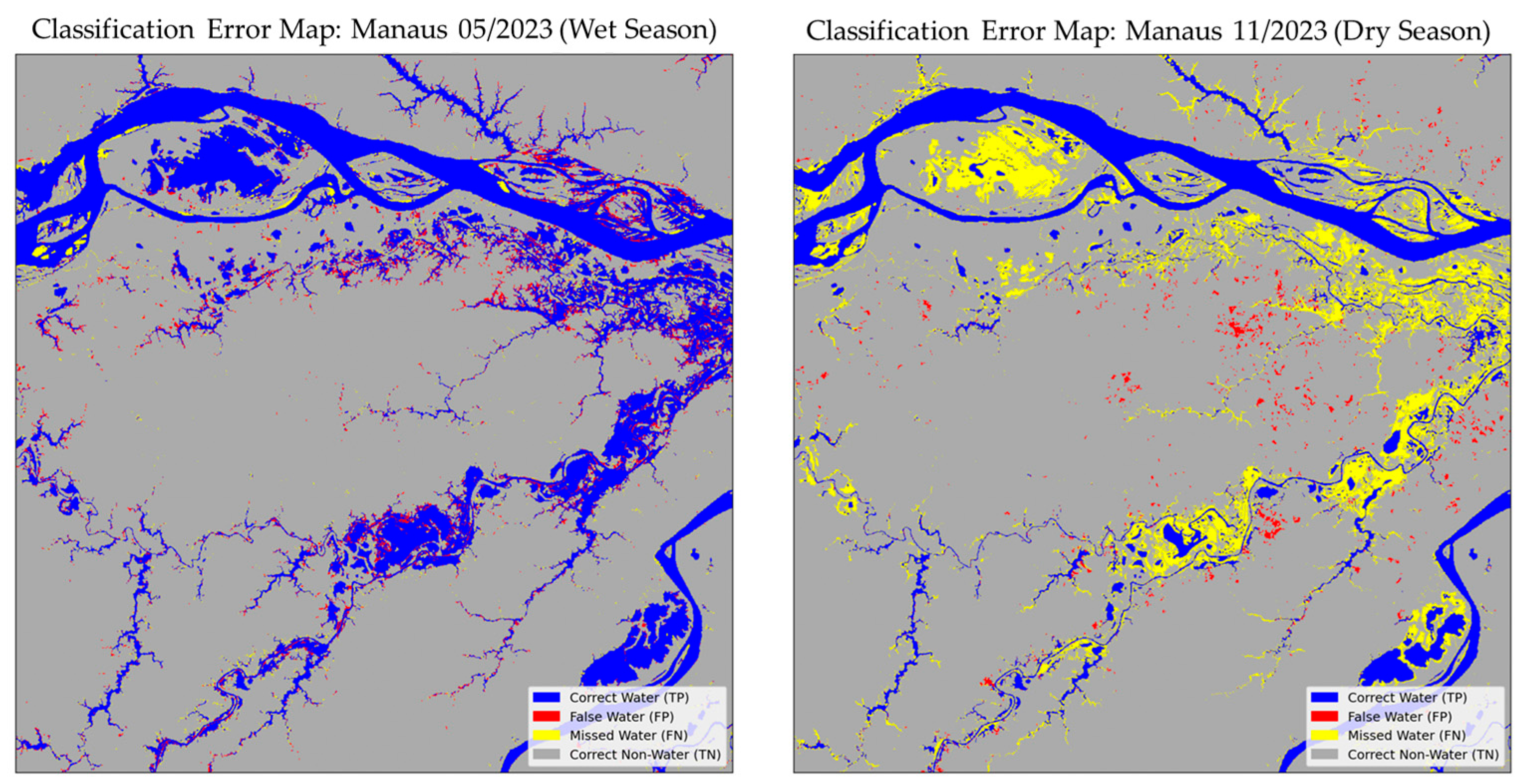
3.3. Water Masking with SAR
3.4. Volume Estimates
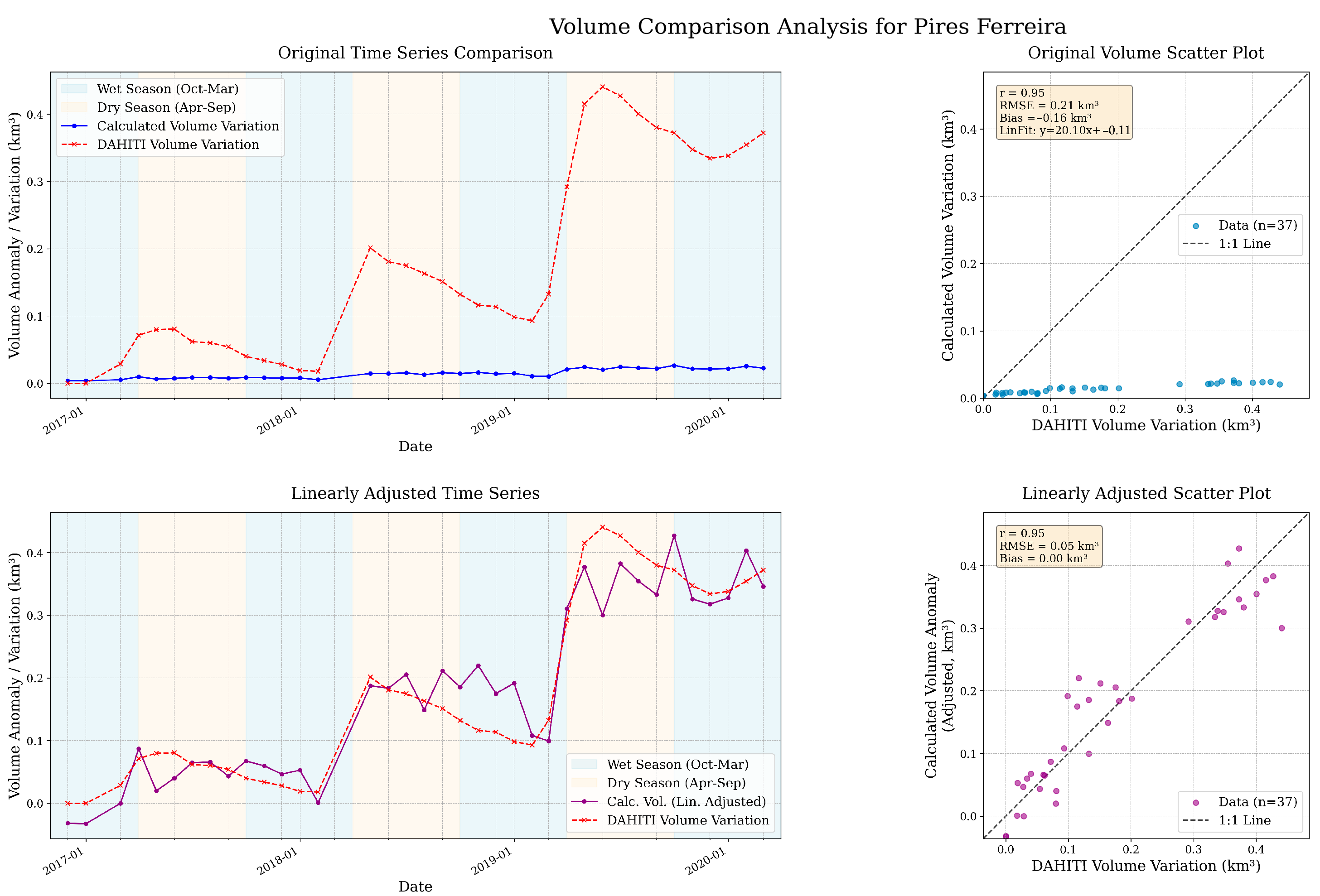
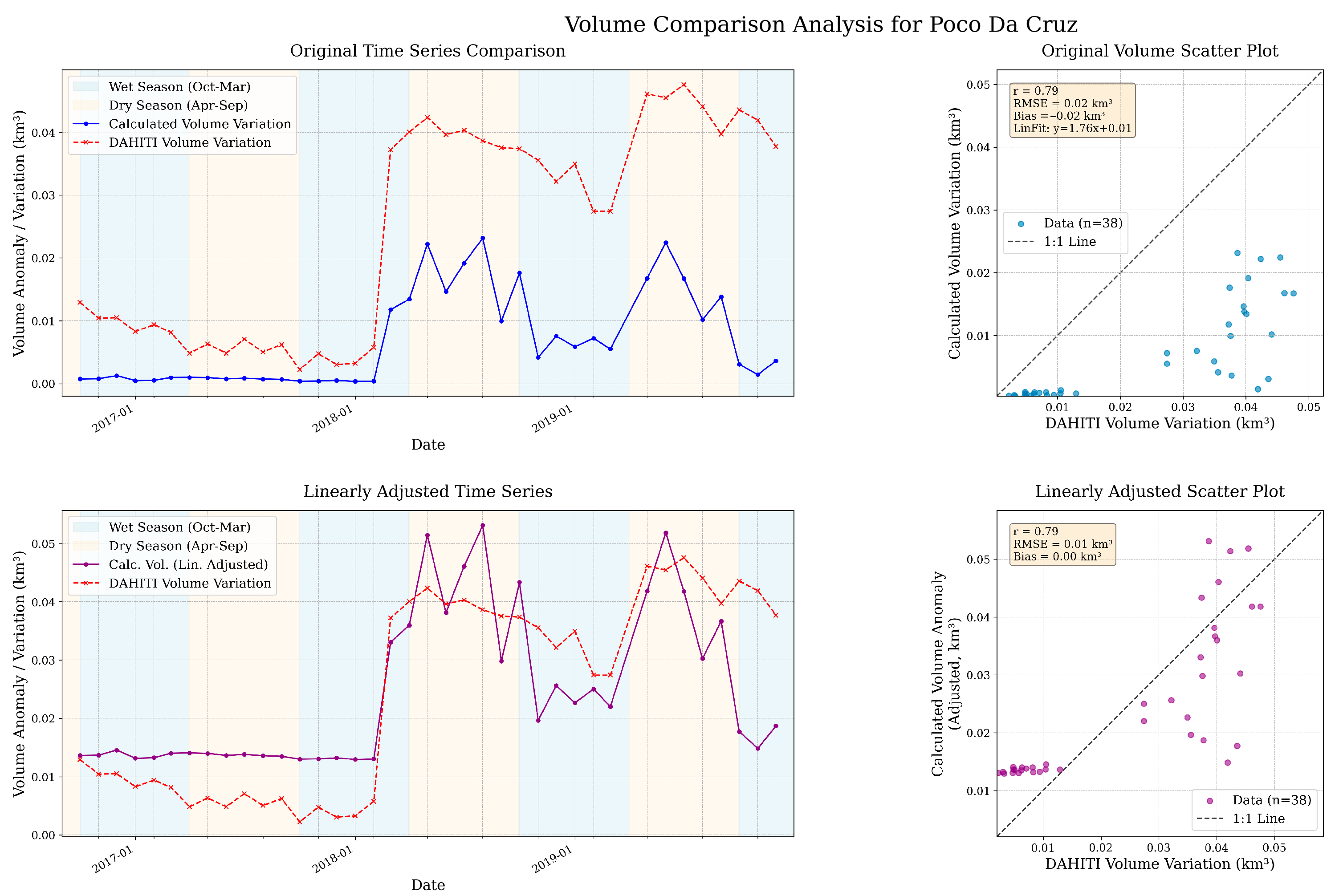
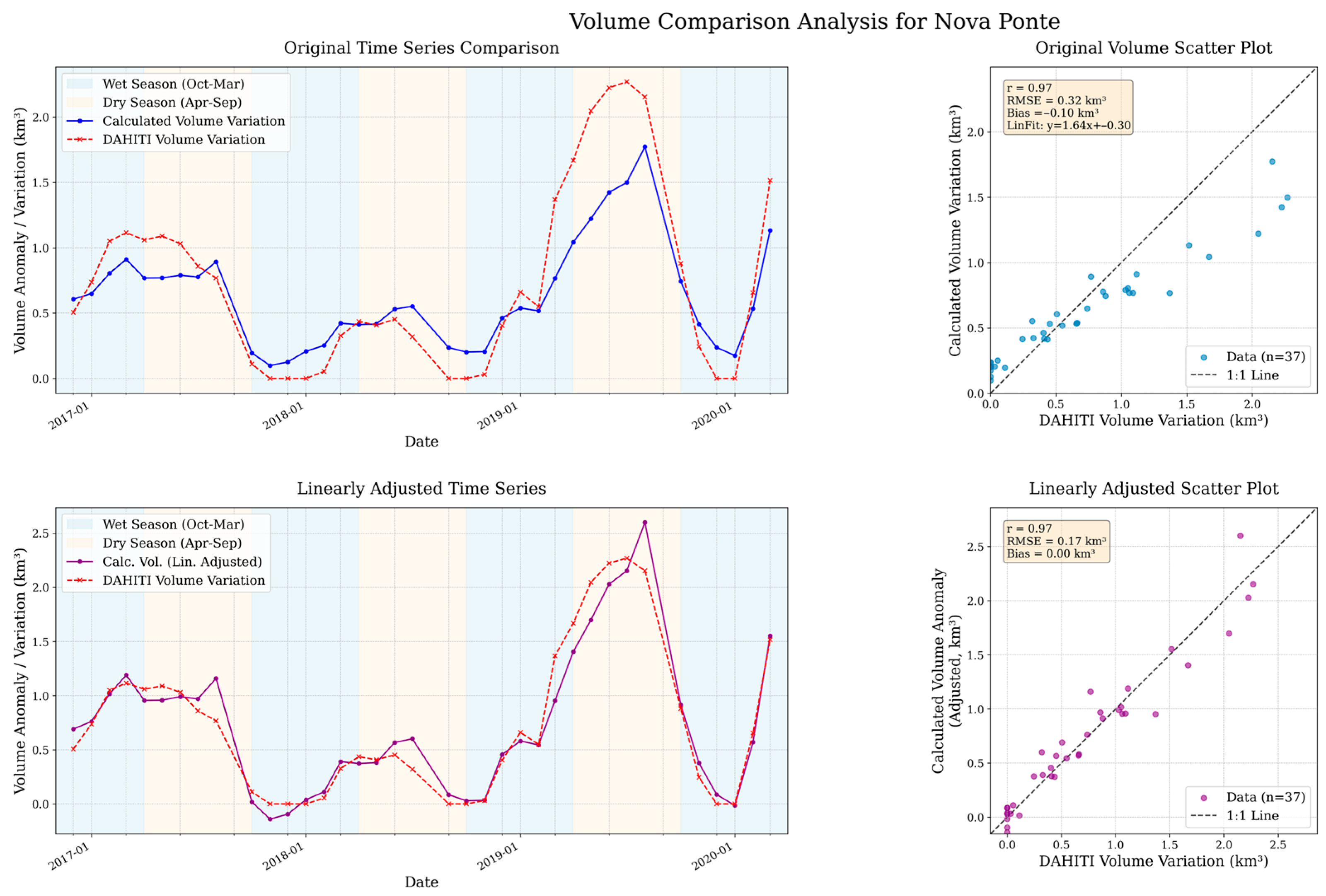
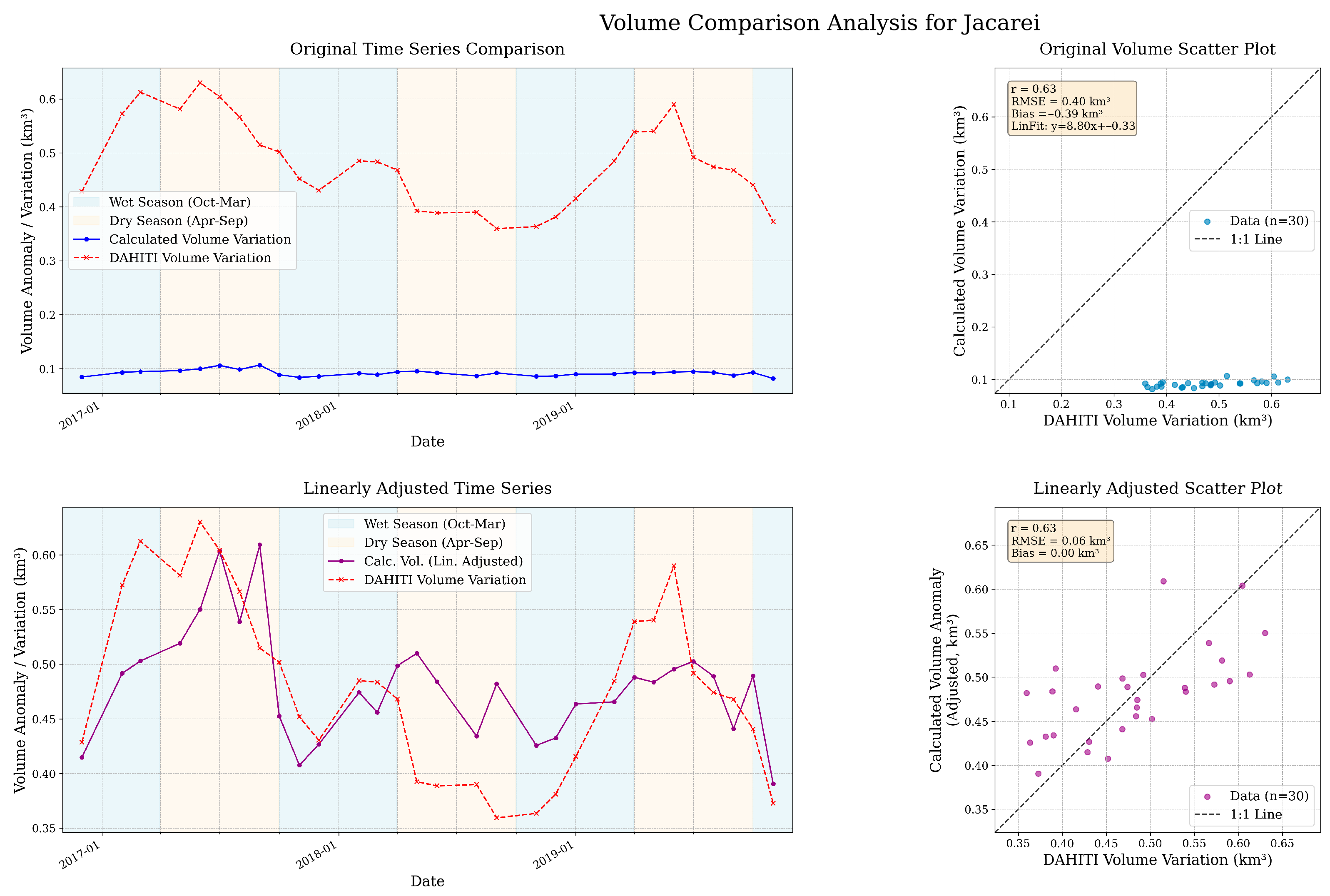
3.4.1. Relative SWV Estimates Comparison at Local Scales
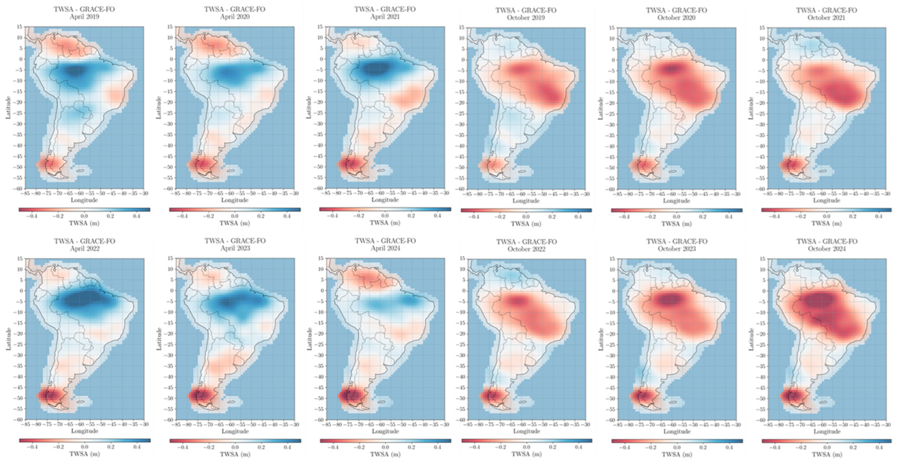
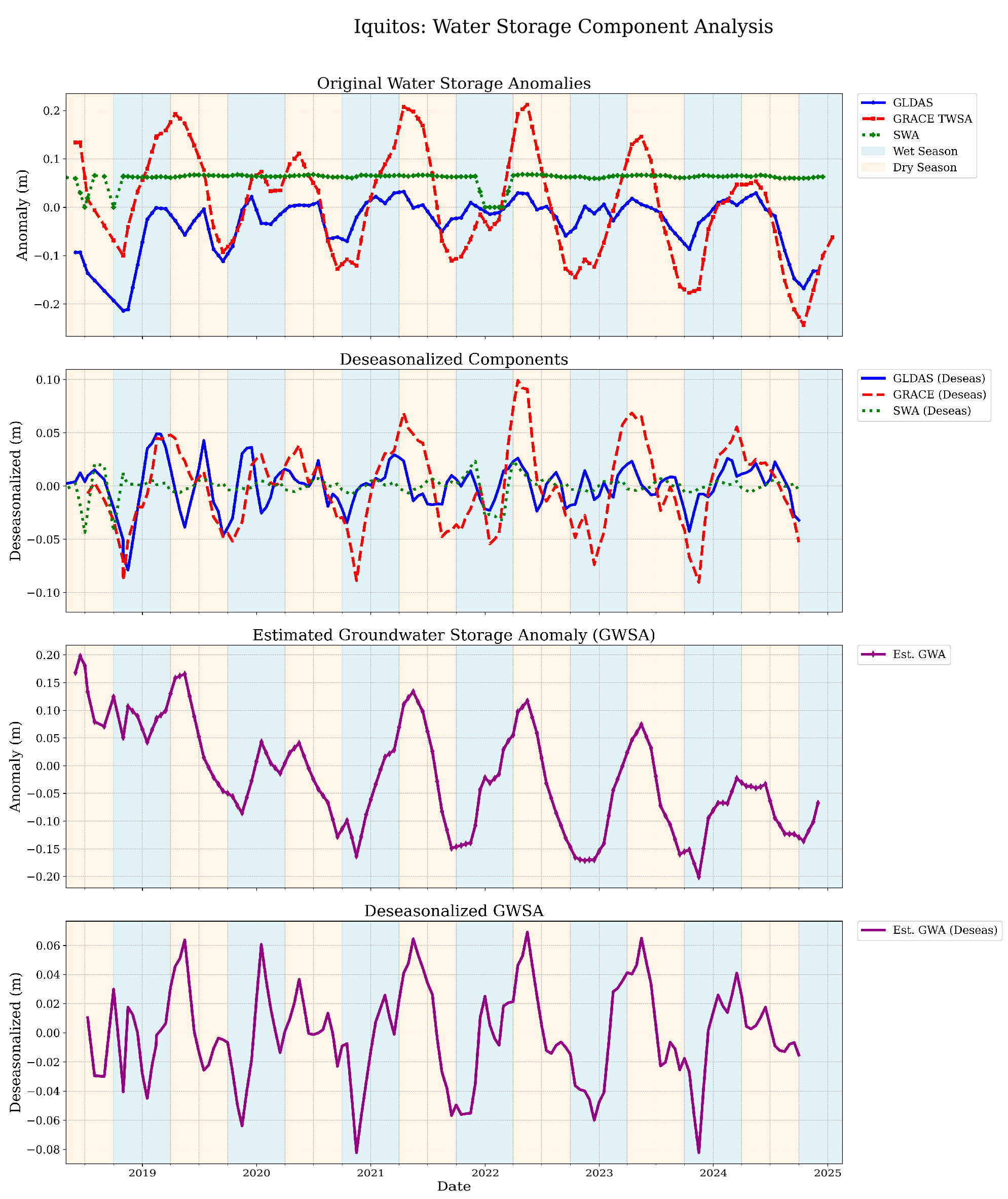
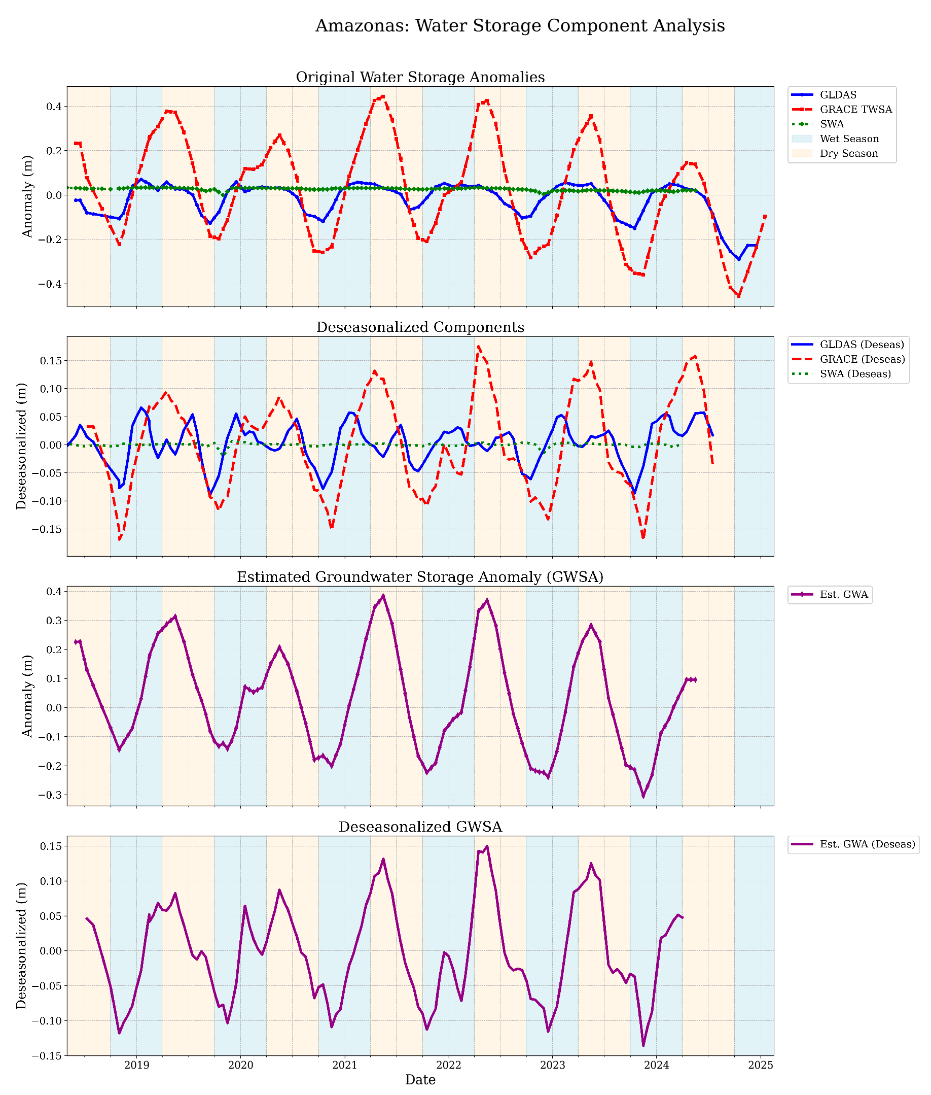
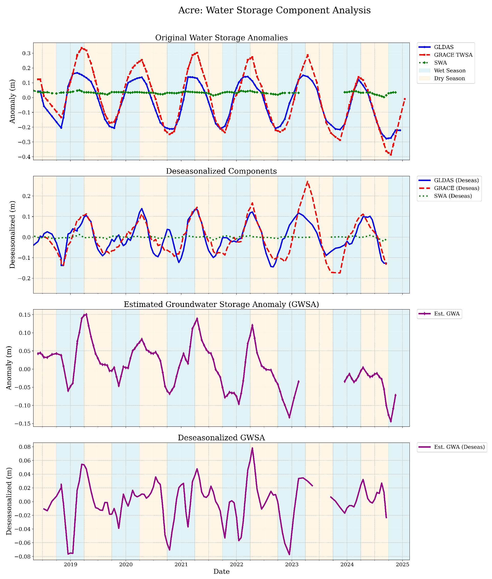
3.4.2. Long-Term SW Storage and GRACE-FO Observations
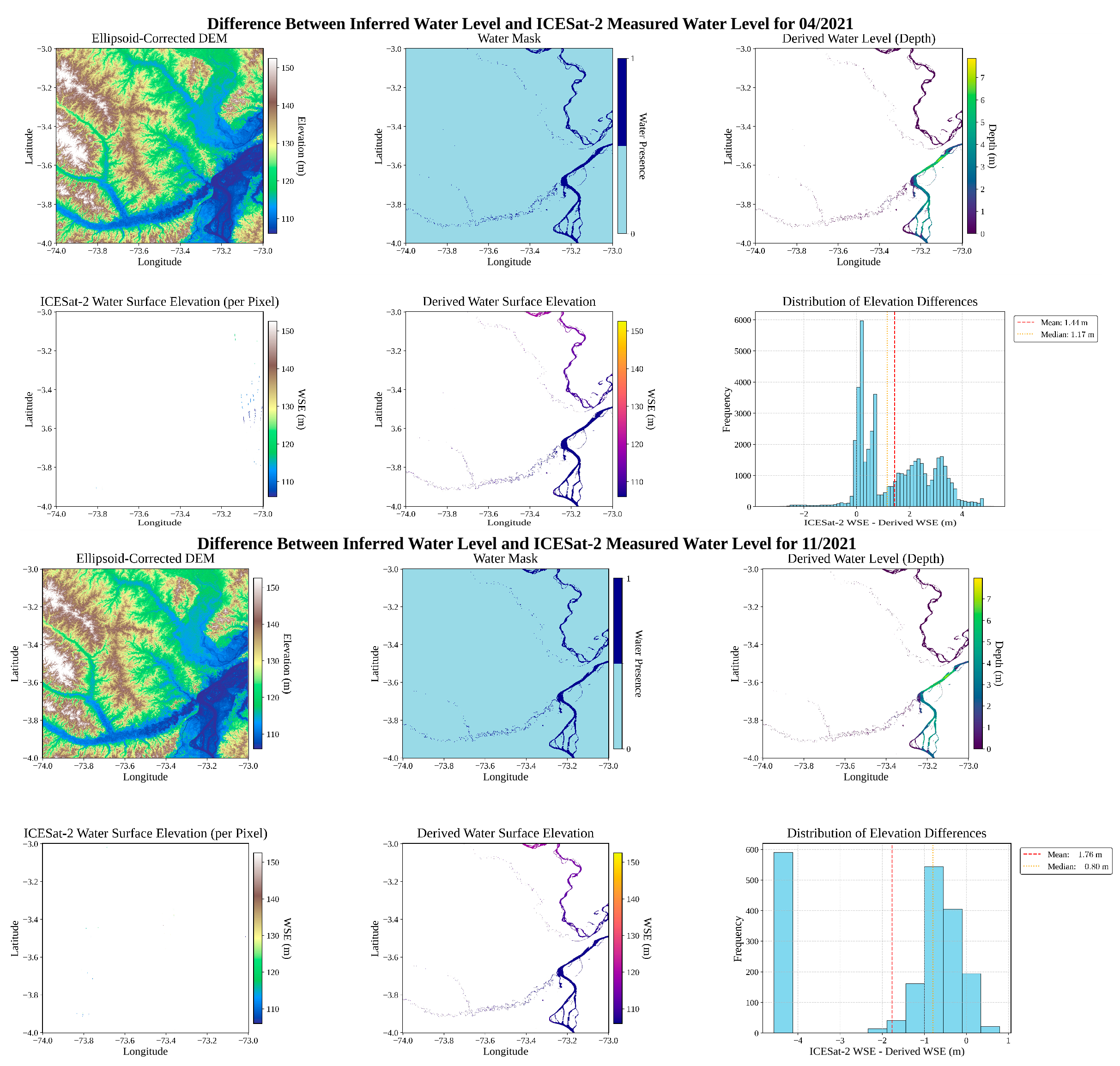
3.4.3. Temporally Coincident Altimetry for SWV Estimates
4. Discussion
5. Conclusions
Author Contributions
Funding
Data Availability Statement
Acknowledgments
Conflicts of Interest
References
- National Research Council. Thriving on Our Changing Planet: A Decadal Strategy for Earth Observation from Space; National Academies Press: Washington, DC, USA, 2018; ISBN 978-0-309-46757-5. [Google Scholar]
- The United Nations World Water Development Report 2024: Water for Prosperity and Peace-UNESCO Digital Library. Available online: https://unesdoc.unesco.org/ark:/48223/pf0000388948 (accessed on 19 February 2025).
- Terrestrial Water Storage (TWS). Available online: https://gcos.wmo.int/site/global-climate-observing-system-gcos/essential-climate-variables/terrestrial-water-storage-tws (accessed on 14 January 2025).
- Save, H.; Bettadpur, S.; Tapley, B.D. High-Resolution CSR GRACE RL05 Mascons. J. Geophys. Res. Solid Earth 2016, 121, 7547–7569. [Google Scholar] [CrossRef]
- Schwatke, C.; Dettmering, D.; Bosch, W.; Seitz, F. DAHITI–an Innovative Approach for Estimating Water Level Time Series over Inland Waters Using Multi-Mission Satellite Altimetry. Hydrol. Earth Syst. Sci. 2015, 19, 4345–4364. [Google Scholar] [CrossRef]
- Yuan, C.; Zhang, F.; Liu, C. A Comparison of Multiple DEMs and Satellite Altimetric Data in Lake Volume Monitoring. Remote Sens. 2024, 16, 974. [Google Scholar] [CrossRef]
- Rezende, I.; Fatras, C.; Oubanas, H.; Gejadze, I.; Malaterre, P.-O.; Peña-Luque, S.; Domeneghetti, A. Reconstruction of Effective Cross-Sections from DEMs and Water Surface Elevation. Remote Sens. 2025, 17, 1020. [Google Scholar] [CrossRef]
- Guenther, E.; Magruder, L.; Neuenschwander, A.; Maze-England, D.; Dietrich, J. Examining CNN Terrain Model for TanDEM-X DEMs Using ICESat-2 Data in Southeastern United States. Remote Sens. Environ. 2024, 311, 114293. [Google Scholar] [CrossRef]
- Cohen, S.; Raney, A.; Munasinghe, D.; Loftis, J.D.; Molthan, A.; Bell, J.; Rogers, L.; Galantowicz, J.; Brakenridge, G.R.; Kettner, A.J.; et al. The Floodwater Depth Estimation Tool (FwDET v2.0) for Improved Remote Sensing Analysis of Coastal Flooding. Nat. Hazards Earth Syst. Sci. 2019, 19, 2053–2065. [Google Scholar] [CrossRef]
- Papa, F.; Frappart, F. Surface Water Storage in Rivers and Wetlands Derived from Satellite Observations: A Review of Current Advances and Future Opportunities for Hydrological Sciences. Remote Sens. 2021, 13, 4162. [Google Scholar] [CrossRef]
- Wang, S.; Li, J.; Russell, H.A.J. Methods for Estimating Surface Water Storage Changes and Their Evaluations. J. Hydrometeorol. 2023, 24, 445–461. [Google Scholar] [CrossRef]
- Di Baldassarre, G.; Schumann, G.; Bates, P.D.; Freer, J.E.; Beven, K.J. Flood-Plain Mapping: A Critical Discussion of Deterministic and Probabilistic Approaches. Hydrol. Sci. J. 2010, 55, 364–376. [Google Scholar] [CrossRef]
- Barichivich, J.; Gloor, E.; Peylin, P.; Brienen, R.J.W.; Schöngart, J.; Espinoza, J.C.; Pattnayak, K.C. Recent Intensification of Amazon Flooding Extremes Driven by Strengthened Walker Circulation. Sci. Adv. 2018, 4, eaat8785. [Google Scholar] [CrossRef]
- Has Climate Change Already Affected ENSO?|NOAA Climate.gov. Available online: http://www.climate.gov/news-features/blogs/enso/has-climate-change-already-affected-enso (accessed on 17 September 2023).
- Del Rio Amador, L.; Boudreault, M.; Carozza, D.A. Global Asymmetries in the Influence of ENSO on Flood Risk Based on 1,600 Years of Hybrid Simulations. Geophys. Res. Lett. 2023, 50, e2022GL102027. [Google Scholar] [CrossRef]
- Espinoza, J.-C.; Marengo, J.A.; Schongart, J.; Jimenez, J.C. The New Historical Flood of 2021 in the Amazon River Compared to Major Floods of the 21st Century: Atmospheric Features in the Context of the Intensification of Floods. Weather Clim. Extrem. 2022, 35, 100406. [Google Scholar] [CrossRef]
- Tadono, T.; Ishida, H.; Oda, F.; Naito, S.; Minakawa, K.; Iwamoto, H. Precise Global DEM Generation by ALOS PRISM. ISPRS Ann. Photogramm. Remote Sens. Spat. Inf. Sci. 2014, II–4, 71–76. [Google Scholar] [CrossRef]
- Uuemaa, E.; Ahi, S.; Montibeller, B.; Muru, M.; Kmoch, A. Vertical Accuracy of Freely Available Global Digital Elevation Models (ASTER, AW3D30, MERIT, TanDEM-X, SRTM, and NASADEM). Remote Sens. 2020, 12, 3482. [Google Scholar] [CrossRef]
- Magruder, L.; Brunt, K.; Neumann, T.; Klotz, B.; Alonzo, M. Passive Ground-Based Optical Techniques for Monitoring the On-Orbit ICESat-2 Altimeter Geolocation and Footprint Diameter. Earth Space Sci. 2021, 8, e2020EA001414. [Google Scholar] [CrossRef]
- Neumann, T.; Brenner, A.; Hancock, D.; Robbins, J.; Saba, J.; Harbeck, K.; Gibbons, A.; Lee, J.; Luthcke, S.; Rebold, T.; et al. ATLAS/ICESat-2 L2A Global Geolocated Photon Data; Version 5 2021; NASA National Snow and Ice Data Center Distributed Active Archive Center: Boulder, CO, USA.
- Neuenschwander, A.; Pitts, K. The ATL08 Land and Vegetation Product for the ICESat-2 Mission. Remote Sens. Environ. 2019, 221, 247–259. [Google Scholar] [CrossRef]
- SlideRule—Sliderule v4.3.1 Documentation. Available online: https://slideruleearth.io (accessed on 18 October 2024).
- ESA-Sentinel-1. Available online: https://www.esa.int/Applications/Observing_the_Earth/Copernicus/Sentinel-1 (accessed on 21 October 2024).
- European Space Agency. Sentinel-2 MSI Level-1C TOA Reflectance; European Space Agency: Paris, France, 2022.
- Keller, M.; Batistella, M.; Gorgens, E.B. LiDAR Survey on 250 Hectares in Jari, Amapá, Brazil, 2021; Brazilian Agricultural Research Corporation (EMBRAPA): Brasilia, Brazil, 2024. [Google Scholar] [CrossRef]
- Keller, M.; Batistella, M.; Gorgens, E.B. LiDAR Survey on 2400 Hectares in São Sebastião Do Uatumã, Amazonas, Brazil, 2021; SIDALC: Turrialba, Costa Rica, 2024. [Google Scholar] [CrossRef]
- Keller, M.; Batistella, M.; Gorgens, E.B. LiDAR Survey on 968 Hectares in GEDI, Mato Grosso, Brazil, 2021; SIDALC: Turrialba, Costa Rica, 2024. [Google Scholar] [CrossRef]
- Keller, M.; Batistella, M.; Gorgens, E.B. LiDAR Survey on 765 Hectares in Tumbira, Pará, Brazil, 2021; SIDALC: Turrialba, Costa Rica, 2024. [Google Scholar] [CrossRef]
- Dos Santos, M.N.; Keller, M.; Batistella, M. LiDAR Survey on 245.7 Hectares in Manaus, Amazonas, Brasil in 2017; SIDALC: Turrialba, Costa Rica, 2023. [Google Scholar] [CrossRef]
- Keller, M.; Batistella, M.; Gorgens, E.B. LiDAR Survey on 1257 Hectares in Reserva Ducke, Amazonas, Brazil, 2021; SIDALC: Turrialba, Costa Rica, 2024. [Google Scholar] [CrossRef]
- Dos-Santos, M.N.; Keller, M.M.; Morton, D.C. LiDAR Surveys over Selected Forest Research Sites, Brazilian Amazon, 2008–2018; ORNL DAAC: Oak RIdge, TN, USA, 2019. [Google Scholar] [CrossRef]
- Magruder, L.; Leigh, H.; Neuenschwander, A. Evaluation of Terrain and Canopy Height Products in Central African Tropical Forests. Int. J. Remote Sens. 2016, 37, 5365–5387. [Google Scholar] [CrossRef]
- Helmer, E.H.; Lefsky, M.A. Forest Canopy Heights in Amazon River Basin Forests as Estimated with the Geoscience Laser Altimeter System (GLAS); USDA Forest Service Proceedings RMRS-P-42CD; U.S. Department of Agriculture, Forest Service, Rocky Mountain Research Station: Fort Collins, CO, USA, 2006.
- Akiba, T.; Sano, S.; Yanase, T.; Ohta, T.; Koyama, M. Optuna: A Next-Generation Hyperparameter Optimization Framework. In Proceedings of the 25th ACM SIGKDD International Conference on Knowledge Discovery & Data Mining, Anchorage, AK, USA, 4–8 August 2019; Association for Computing Machinery: New York, NY, USA, 2019; pp. 2623–2631. [Google Scholar]
- Sentinel-1 Algorithms|Google Earth Engine. Available online: https://developers.google.com/earth-engine/guides/sentinel1 (accessed on 30 October 2024).
- White, L.; Brisco, B.; Dabboor, M.; Schmitt, A.; Pratt, A. A Collection of SAR Methodologies for Monitoring Wetlands. Remote Sens. 2015, 7, 7615–7645. [Google Scholar] [CrossRef]
- Tarpanelli, A.; Mondini, A.C.; Camici, S. Effectiveness of Sentinel-1 and Sentinel-2 for Flood Detection Assessment in Europe. Nat. Hazards Earth Syst. Sci. 2022, 22, 2473–2489. [Google Scholar] [CrossRef]
- Gulácsi, A.; Kovács, F. Sentinel-1-Imagery-Based High-Resolution Water Cover Detection on Wetlands, Aided by Google Earth Engine. Remote Sens. 2020, 12, 1614. [Google Scholar] [CrossRef]
- Otsu, N. A Threshold Selection Method from Gray-Level Histograms. IEEE Trans. Syst. Man Cybern. 1979, 9, 62–66. [Google Scholar] [CrossRef]
- Pires Ferreira, Reservoir|General Info|Database for Hydrological Time Series of Inland Waters (DAHITI). Available online: https://dahiti.dgfi.tum.de/en/8671/ (accessed on 26 February 2025).
- Poço Da Cruz, Reservoir|General Info|Database for Hydrological Time Series of Inland Waters (DAHITI). Available online: https://dahiti.dgfi.tum.de/en/8702/ (accessed on 26 February 2025).
- Nova Ponte, Reservoir|General Info|Database for Hydrological Time Series of Inland Waters (DAHITI). Available online: https://dahiti.dgfi.tum.de/en/10351/ (accessed on 26 February 2025).
- Jacarei, Reservoir|General Info|Database for Hydrological Time Series of Inland Waters (DAHITI). Available online: https://dahiti.dgfi.tum.de/en/10345/ (accessed on 26 February 2025).
- Monthly Gridded Global Land Data Assimilation System (GLDAS) from Noah-v3.3 Land Hydrology Model for GRACE and GRACE-FO over Nominal Months. Available online: https://podaac.jpl.nasa.gov/dataset/TELLUS_GLDAS-NOAH-3.3_TWS-ANOMALY_MONTHLY (accessed on 22 January 2025).
- Cooley, S.W.; Smith, L.C.; Stepan, L.; Mascaro, J. Tracking Dynamic Northern Surface Water Changes with High-Frequency Planet CubeSat Imagery. Remote Sens. 2017, 9, 1306. [Google Scholar] [CrossRef]
- Pekel, J.-F.; Cottam, A.; Gorelick, N.; Belward, A.S. High-Resolution Mapping of Global Surface Water and Its Long-Term Changes. Nature 2016, 540, 418–422. [Google Scholar] [CrossRef]
- MapBiomas Amazonía Project. Collection 6 of Annual Land Cover and Land Use Maps, Version 1. Available online: https://amazonia.mapbiomas.org/ (accessed on 11 May 2025).
- Hess, L.L.; Melack, J.M.; Affonso, A.G.; Barbosa, C.; Gastil-Buhl, M.; Novo, E.M.L.M. Wetlands of the Lowland Amazon Basin: Extent, Vegetative Cover, and Dual-Season Inundated Area as Mapped with JERS-1 Synthetic Aperture Radar. Wetlands 2015, 35, 745–756. [Google Scholar] [CrossRef]
- Pedreros-Guarda, M.; Abarca-del-Río, R.; Crétaux, J.F.; Paris, A. Long-Term Lake Water Levels in Central Chile Using Satellite Altimetry and Conceptual Hydrological Modelling Approaches. Adv. Space Res. 2025, in press. [Google Scholar] [CrossRef]
- Jesus, J.; Kuplich, T. Applications of SAR Data to the Estimate of Forest Biophysical Variables in Brazil. Cerne 2020, 26, 88. [Google Scholar] [CrossRef]
- Quick Facts|Mission. Available online: https://nisar.jpl.nasa.gov/mission/quick-facts (accessed on 31 December 2024).
- Zhang, Z.; Bo, Y.; Jin, S.; Chen, G.; Dong, Z. Dynamic Water Level Changes in Qinghai Lake from Integrating Refined ICESat-2 and GEDI Altimetry Data (2018–2021). J. Hydrol. 2023, 617, 129007. [Google Scholar] [CrossRef]


| Feature Name | Source | Description |
|---|---|---|
| Ground-Classified Photon Heights | ICESat-2 ATL03 | Height measurements of ground-classified photon returns (terrain). |
| Distance to Coast | AW3D30 | Proximity to coastal region. |
| DEM Height | AW3D30 | Height measurement of DEM. |
| Terrain Slope | AW3D30 | Rate of elevation change. |
| Vegetation Cover | Sentinel-1 GRD | SAR-based classification of vegetation density. |
| EVI | Sentinel-2 MSI | Enhanced Vegetation Index, assessing vegetation health and coverage. |
| NDVI | Sentinel-2 MSI | Normalized Difference Vegetation Index, assessing vegetation health and coverage. |
| VV Standard Deviation | Sentinel-1 GRD | Variability in vertical transmit/receive polarization, used to assess roughness. |
| VH Standard Deviation | Sentinel-1 GRD | Variability in vertical transmit/receive polarization, used to assess vegetation. |
| Location (X,Y,Z) | Coordinate data in Cartesian coordinates | Spatial representation of points converted to avoid distortion. |
| Reservoir | Latitude | Longitude | Avg Area [km2] | Date Overlap |
|---|---|---|---|---|
| Pires Ferreira | −4.225° | −40.4487° | 44.454 | 2016-12 to 2020-03 |
| Poço da Cruz | −8.4973° | −37.681° | 22.607 | 2016-10 to 2019-12 |
| Nova Ponte | −19.1291° | −47.3831° | 276.11 | 2016-12 to 2020-03 |
| Jacareí | −22.968° | −46.3516° | 34.718 | 2016-12 to 2019-11 |
| ROI | Min Latitude | Max Latitude | Min Longitude | Max Longitude |
|---|---|---|---|---|
| Iquitos | −4.0° | −3.0° | −74.0° | −73.0° |
| Amazonas | −5.0° | −4.0° | −69.0° | −68.0° |
| Acre | −10.0° | −9.0° | −68.0° | −67.0° |
| Manaus | −4.0° | −3.0° | −60.0° | −59.0° |
| Dataset | Model | Points | Test RMSE (m) | Test MAE (m) | Test MAPE (%) | Holdout RMSE (m) | CV RMSE Mean (m) | Runtime (s) |
|---|---|---|---|---|---|---|---|---|
| Model 1 (subset) | Gradient Boosting | 400,000 | 24.8143 | 16.9337 | 37.1727 | 32.9318 | 25.6186 | 1101.7 |
| Ridge | 400,000 | 25.1981 | 16.6244 | 42.3386 | 33.1267 | 27.9791 | 0.64 | |
| LGBM | 400,000 | 25.4732 | 17.3843 | 32.6046 | 40.1545 | 21.1549 | 144.95 | |
| Extra Trees | 400,000 | 25.6704 | 17.764 | 32.4216 | 36.2144 | 20.7149 | 200.36 | |
| Lasso | 400,000 | 26.1356 | 16.984 | 53.7819 | 33.3548 | 28.7234 | 2.81 | |
| ElasticNet | 400,000 | 26.8239 | 17.3842 | 56.0406 | 33.9216 | 29.5481 | 1.99 | |
| CatBoost | 400,000 | 29.5375 | 20.2909 | 24.0245 | 43.4658 | 18.3456 | 132.39 | |
| XGBoost | 400,000 | 29.7489 | 20.2821 | 25.4909 | 39.7076 | 17.827 | 7.75 | |
| RandomForest | 400,000 | 30.7209 | 20.9816 | 35.9711 | 39.6489 | 13.7533 | 3647.28 | |
| Model 2 | Extra Trees | 18,805 | 1.4684 | 0.7352 | 0.1261 | 1.679 | 1.8851 | 4.53 |
| RandomForest | 18,805 | 1.5718 | 0.8073 | 0.1318 | 1.946 | 1.9714 | 45.9 | |
| XGBoost | 18,805 | 1.8431 | 1.1379 | 0.2507 | 2.1834 | 2.2182 | 1.01 | |
| LGBM | 18,805 | 2.1521 | 1.3565 | 0.354 | 2.4626 | 2.3754 | 2.89 | |
| CatBoost | 18,805 | 2.2152 | 1.5176 | 0.4297 | 2.4711 | 2.642 | 19.7 | |
| Gradient Boosting | 18,805 | 2.5266 | 1.6664 | 0.4748 | 2.8236 | 2.7969 | 16.84 | |
| Ridge | 18,805 | 6.4828 | 4.7891 | 2.1388 | 6.3496 | 6.3454 | 0.13 | |
| Lasso | 18,805 | 8.9525 | 6.3691 | 3.1299 | 9.0292 | 8.7669 | 0.44 | |
| ElasticNet | 18,805 | 36.7624 | 29.1 | 14.2088 | 36.0068 | 36.5794 | 0.19 |
| Metric | Pre-Model 1 | Post-Model 1 | Percent Improvement |
|---|---|---|---|
| RMSE (m) | 34.01 (11.95%) | 11.38 (4%) | 66.53% |
| MAE (m) | 22.64 (7.95%) | 7.37 (2.59%) | 67.43% |
| MAPE (%) | 14.13% | 4.24% | 70.01% |
| Metric | Pre-Model 2 | Post-Model 2 | Percent Improvement |
|---|---|---|---|
| RMSE (m) | 9.32 (1.7%) | 1.978 (0.36%) | 78.78% |
| MAE (m) | 6.08 (1.11%) | 0.93 (0.17%) | 84.71% |
| MAPE (%) | 3.46% | 0.17% | 95.09% |
| ROI | ICESat-2 Coverage (%) | Initial RMSE (m) | Final RMSE (m) | Initial MAE (m) | Final MAE (m) | Initial MAPE (%) | Final MAPE (%) |
|---|---|---|---|---|---|---|---|
| Acre | 10.84% | 11.06 | 4.19 | 7.28 | 3.00 | 3.92% | 1.73% |
| Amazonas | 2.04% | 16.14 | 2.74 | 13.82 | 1.71 | 12.20% | 1.75% |
| Manaus | 23.97% | 9.63 | 2.86 | 6.99 | 2.11 | 226.63% * | 3.01% |
| Iquitos | 6.19% | 13.43 | 2.49 | 10.61 | 1.63 | 8.03% | 1.39% |
| Pires Ferreira | 0.41% | 31.59 | 1.39 | 31.53 | 1.01 | 17.20% | 0.66% |
| Nova Ponte | 9.12% | 23.16 | 3.14 | 22.65 | 2.10 | 2.44% | 0.30% |
| Poço da Cruz | 2.77% | 19.21 | 1.21 | 19.16 | 0.79 | 4.23% | 0.18% |
| Jacareí | 0.71% | 10.50 | 4.55 | 8.897 | 2.63 | 1.03% | 0.30% |
| Metric | Season | Mean ± Std |
|---|---|---|
| F1_Score | Dry | 0.805 ± 0.075 |
| F1_Score | Wet | 0.819 ± 0.081 |
| Iou_Jaccard | Dry | 0.679 ± 0.098 |
| Iou_Jaccard | Wet | 0.700 ± 0.100 |
| Precision | Dry | 0.898 ± 0.102 |
| Precision | Wet | 0.911 ± 0.091 |
| Recall | Dry | 0.745 ± 0.111 |
| Recall | Wet | 0.756 ± 0.102 |
| Reservoir | Initial RMSE (km3) | Adjusted RMSE (km3) | Initial MAE (km3) | Adjusted MAE (km3) | Pearson’s Correlation Coefficient | p-Value |
|---|---|---|---|---|---|---|
| Pires Ferreira | 0.2147 | 0.0461 | 0.1647 | 0.0364 | 0.9478 | 0.0000 |
| Poço da Cruz | 0.0211 | 0.0102 | 0.0176 | 0.0084 | 0.7914 | 0.0000 |
| Nova Ponte | 0.3215 | 0.1681 | 0.2406 | 0.1216 | 0.9687 | 0.0000 |
| Jacareí | 0.3964 | 0.0612 | 0.3891 | 0.0506 | 0.6347 | 0.0002 |
| ROI | Trend GRACE-FO TWS (m/yr) | p-Value GRACE-FO TWS Trend | Trend GLDAS (m/yr) | p-Value GLDAS Trend | Trend SWS (m/yr) | p-Value SWS Trend | Trend Est. GWS (m/yr) | p-Value Est. GWS Trend |
|---|---|---|---|---|---|---|---|---|
| Iquitos | −0.0217 | 0 | −0.0022 | 0 | −0.0014 | 0.0095 | −0.0287 | 0 |
| Manaus | −0.0468 | 0.0034 | −0.0021 | 0.0299 | −0.0032 | 0.1919 | −0.0218 | 0.0223 |
| Acre | −0.0346 | 0 | −0.0033 | 0.0034 | −0.0013 | 0 | −0.0169 | 0 |
| Amazonas | −0.0326 | 0.0008 | −0.0018 | 0.0011 | −0.0022 | 0 | −0.0209 | 0.0135 |
| ROI | RMSE (GRACE-FO vs. Sum) (m) | Bias (GRACE-FO—Sum) (m) | Corr (GRACE-FO SWA) | Corr (GRACE-FO GLDAS) | Corr (GLDAS SWA) |
|---|---|---|---|---|---|
| Iquitos | 0.0959 | −0.0215 | 0.0917 | 0.524 | 0.1643 |
| Manaus | 0.3102 | −0.2153 | 0.821 | 0.8178 | 0.4635 |
| Acre | 0.0619 | 0.0065 | 0.5947 | 0.9623 | 0.6303 |
| Amazonas | 0.177 | 0.0303 | 0.5577 | 0.7027 | 0.3569 |
Disclaimer/Publisher’s Note: The statements, opinions and data contained in all publications are solely those of the individual author(s) and contributor(s) and not of MDPI and/or the editor(s). MDPI and/or the editor(s) disclaim responsibility for any injury to people or property resulting from any ideas, methods, instructions or products referred to in the content. |
© 2025 by the authors. Licensee MDPI, Basel, Switzerland. This article is an open access article distributed under the terms and conditions of the Creative Commons Attribution (CC BY) license (https://creativecommons.org/licenses/by/4.0/).
Share and Cite
Renshaw, M.; Magruder, L.A. Advancing Scalable Methods for Surface Water Monitoring: A Novel Integration of Satellite Observations and Machine Learning Techniques. Geosciences 2025, 15, 255. https://doi.org/10.3390/geosciences15070255
Renshaw M, Magruder LA. Advancing Scalable Methods for Surface Water Monitoring: A Novel Integration of Satellite Observations and Machine Learning Techniques. Geosciences. 2025; 15(7):255. https://doi.org/10.3390/geosciences15070255
Chicago/Turabian StyleRenshaw, Megan, and Lori A. Magruder. 2025. "Advancing Scalable Methods for Surface Water Monitoring: A Novel Integration of Satellite Observations and Machine Learning Techniques" Geosciences 15, no. 7: 255. https://doi.org/10.3390/geosciences15070255
APA StyleRenshaw, M., & Magruder, L. A. (2025). Advancing Scalable Methods for Surface Water Monitoring: A Novel Integration of Satellite Observations and Machine Learning Techniques. Geosciences, 15(7), 255. https://doi.org/10.3390/geosciences15070255