On Applicability of the Radially Integrated Geopotential in Modelling Deep Mantle Structure

Abstract

A long-wavelength geoidal geometry reflects mainly lateral density variations in the Earth’s mantle, with the most pronounced features of the Indian Ocean Geoid Low and the West Pacific and North Atlantic Geoid Highs. Despite this spatial pattern being clearly manifested in the global geoidal geometry determined from gravity-dedicated satellite missions, the gravitational signature of the deep mantle could be refined by modelling and subsequently removing the gravitational contribution of lithospheric geometry and density structure. Nonetheless, the expected large uncertainties in available lithospheric density models (CRUST1.0, LITHO1.0) limit, to some extent, the possibility of realistically reproducing the gravitational signature of the deep mantle. To address this issue, we inspect an alternative approach. Realizing that the gravity geopotential field (i.e., gravity potential) is smoother than its gradient (i.e., gravity), we apply the integral operator to geopotential and then investigate the spatial pattern of this functional (i.e., radially integrated geopotential). Results show that this mathematical operation enhances a long-wavelength signature of the deep mantle by filtering out the gravitational contribution of the lithosphere. This finding is explained by the fact that in the definition of this functional, spherical harmonics of geopotential are scaled by the factor 1/n (where n is the degree of spherical harmonics), thus lessening the contribution of higher-degree spherical harmonics in the radially integrated geopotential. We also demonstrate that further enhancement of the mantle signature in this functional could be achieved based on modelling and subsequent removal of the gravitational contribution of lithospheric geometry and density structure.

1. Introduction

Since seismic surveys are still sparse and uneven in many parts of the world, remote-sensing data acquired from synthetic-aperture radars, satellite altimetry, and dedicated satellite-gravity missions have been used in numerous regional and global studies of the Earth’s interior. For instance, studies of the global geoid pattern helped scientists better understand a deep mantle structure mainly manifested in a long-wavelength geoidal geometry (e.g., [1,2,3,4,5,6,7,8,9,10,11]). Gravity-dedicated satellite missions could recover the Earth’s gravitational field with a spatial resolution up to ~80 km (in terms of a half-wavelength at the equator), while further refinement has been achieved by integrating ground-based, air-borne, and sea-borne gravity measurements as well as marine gravity data from satellite altimetry (e.g., [12]).

In the Earth’s interior studies, gravity information together with topographic, bathymetric, and ice-thickness datasets and additional geophysical and geological constraints are often used to investigate geological and tectonic settings within the upper lithosphere (e.g., [13,14,15,16,17,18,19]). The long-wavelength geoidal undulations are, on the other hand, more suitable to study deeper structures in the mantle (cf. [20]) because the global geoidal geometry comprises mainly a long-wavelength signature of mantle density structure. In contrast, the global gravity pattern better exhibits lithospheric signature.

Although the signature of lithospheric structure is partially filtered out in the geoidal geometry, the gravimetric interpretation of deep mantle density structure could further be improved by modelling and subtracting the lithospheric signature. The CRUST1.0 [21] and LITHO1.0 [22] lithospheric density models have been used for this purpose [23]. Nonetheless, the current lithospheric density models have restricted accuracy and resolution. Different methods were, therefore, proposed based on applying spectral decomposition and filtering techniques or using isostatic models to enhance a long-wavelength signature of deeper sources in the geoidal geometry and gravity pattern. Besides, isostatic theories have limitations to realistically model real compensation mechanisms within parts of the lithosphere that are not in isostatic equilibrium, such as active orogenic belts, divergent tectonic margins, and active volcanic formations. Spectral decomposition and filtering techniques are, on the other hand, also inadequate because separation of gravitational sources at different depths is not unique.

To address the theoretical and practical limitations of the above methods, we inspect the possibility of enhancing the gravitational signature of the deep mantle by applying the radial integral of geopotential. Whereas the geopotential (or equivalently geoidal) geometry has a prevailing long-wavelength pattern attributed to mantle structure, its radial derivative (i.e., gravity) exhibits a more detailed gravitational signature of lithospheric geometry and density structure. Consequently, the application of the integral operator to geopotential filters out lithospheric pattern while enhancing the signature of the deep mantle because spherical harmonics of geopotential are scaled by the factor 1/n. We then apply gravimetric forward modelling techniques to model the gravitational contribution of lithospheric geometry and density structure, remove this contribution from the geopotential and its radial integral, and compare both results with the mantle model.

2. Theory

In this section, we first define the radial integral of disturbing potential, which is obtained from the geopotential (i.e., actual gravity potential) after subtracting the normal gravity potential. We then provide definitions of respective gravitational corrections to this functional that are applied to mathematically model and remove the gravitational signature of lithospheric geometry and density structure.

2.1. Radial Integral of Earth’s Disturbing Potential

The radial integral of the disturbing potential is defined by [24]

$$\Im ={\displaystyle \underset{r}{\int }T\left(r,\mathsf{\Omega }\right)} \mathrm{d}r$$

(1)

where T denotes the disturbing potential, i.e., the difference between the actual gravity potential W and the normal gravity potential U (T = W − U). The 3-D position in Equation (1) and thereafter is defined in the spherical coordinate system $(r,\mathsf{\Omega })$, where $r$ is the radius and $\mathsf{\Omega }=(\varphi ,\lambda )$ denotes the spherical direction with the spherical latitude $\varphi$ and longitude $\lambda$. The spherical harmonic representation of the Earth’s disturbing potential T reads (e.g., [25])

$$T\left(r,\mathsf{\Omega }\right)={\displaystyle \frac{\mathrm{GM}}{\mathrm{R}}} {\displaystyle \sum _{n=2}^{\infty }{\left(\frac{\mathrm{R}}{r}\right)}^{n+1}} {\displaystyle \sum _{m=-n}^n{\mathrm{T}}_{\mathrm{n},\mathrm{m}} {\mathrm{Y}}_{\mathrm{n},\mathrm{m}}\left(\mathsf{\Omega }\right)}$$

(2)

where $T_{n,m}$ are (fully-normalized) numerical coefficients of the disturbing potential T of degree n and order m, and the (fully-normalized) surface spherical functions $Y_{n,m}$ are defined by

$${\mathrm{Y}}_{\mathrm{n},\mathrm{m}}\left(\mathsf{\Omega }\right)={\mathrm{P}}_{\mathrm{n},\mathrm{m}}\left(\sin \varphi \right)\left\{\begin{array}{c}\cos m \lambda \hspace{1em}m\ge 0\\ \sin \left|m\right|\lambda \hspace{1em}m<0\end{array}\right.$$

(3)

with $P_{n,m}$ denoting the (fully-normalized) associated Legendre functions. Combining Equations (1) and (2), the spherical harmonic representation of the radial integral of Earth’s disturbing potential is given by

$${\displaystyle \int T \mathrm{d}r}={\displaystyle \frac{\mathrm{GM}}{\mathrm{R}}} {\displaystyle \sum _{n=2}^{\infty }{\displaystyle \int {\left(\frac{\mathrm{R}}{r}\right)}^{n+1} \mathrm{d}r}} {\displaystyle \sum _{m=-n}^n{\mathrm{T}}_{\mathrm{n},\mathrm{m}} {\mathrm{Y}}_{\mathrm{n},\mathrm{m}}\left(\mathsf{\Omega }\right)}={\displaystyle \frac{\mathrm{GM}}{\mathrm{R}}} {\displaystyle \sum _{n=2}^{\infty }{\mathrm{R}}^{n+1}{\displaystyle \int r^{-n-1} \mathrm{d}r}} {\displaystyle \sum _{m=-n}^n{\mathrm{T}}_{\mathrm{n},\mathrm{m}} {\mathrm{Y}}_{\mathrm{n},\mathrm{m}}\left(\mathsf{\Omega }\right)}$$

(4)

The radial integral of $r^{-n-1}$ on the right-hand side of Equation (4) is given by

$${\displaystyle \int r^{-n-1} \mathrm{d}r}=-{\displaystyle \frac{1}{n}}{r}^{-n}+\mathrm{C}\hspace{1em}\hspace{1em}\left(n>0\right)$$

(5)

Substitution from Equation (5) back to Equation (4) yields

$${\displaystyle \int T \mathrm{d}r}=-\mathrm{GM} {\displaystyle \sum _{n=2}^{\infty }{\mathrm{R}}^n\left(\frac{r^{-n}}{n}+\mathrm{C}\right)} {\displaystyle \sum _{m=-n}^n{\mathrm{T}}_{\mathrm{n},\mathrm{m}} {\mathrm{Y}}_{\mathrm{n},\mathrm{m}}\left(\mathsf{\Omega }\right)}$$

(6)

Setting the integral constant C = 0, the indefinite radial integral of Earth’s disturbing potential in Equation (6) becomes

$${\displaystyle \int T \mathrm{d}r}=-\mathrm{GM} {\displaystyle \sum _{n=2}^{\infty }\frac{1}{n}{\left(\frac{\mathrm{R}}{r}\right)}^n} {\displaystyle \sum _{m=-n}^n{\mathrm{T}}_{\mathrm{n},\mathrm{m}} {\mathrm{Y}}_{\mathrm{n},\mathrm{m}}\left(\mathsf{\Omega }\right)}$$

(7)

As seen in the definition of the radial integral of disturbing potential in Equation (7), the spherical harmonics of disturbing potential are scaled by 1/n, thus effectively filtering out the contribution from higher-degree harmonic terms. Depending on the accuracy of available global lithospheric density models, further enhancement of the mantle signature in the radially integrated disturbing potential could be done by modelling and removing the gravitational contribution of lithospheric geometry and density structure. This mathematical procedure is realized in several numerical steps described below.

2.2. Radial Integral of Bouguer Disturbing Potential

The radial integral of the Bouguer disturbing potential T^B is introduced in the following form

$${\Im }^B={\displaystyle \underset{r}{\int }{T}^B} \mathrm{d}r$$

(8)

The Bouguer disturbing potential T^B reads

$$T^{\mathrm{B}}=T-V^T-V^B-V^I$$

(9)

where V^T is the gravitational potential of topographic masses (i.e., the topographic potential), V^B is the gravitational potential of ocean density contrast (i.e., the bathymetric potential), and V^I is the gravitational potential of polar glaciers’ ice density contrast (i.e., the ice potential).

Substituting from Equation (9) back into Equation (8), we arrive at

$${\Im }^B={\displaystyle \underset{r}{\int }T} \mathrm{d}r-{\displaystyle \underset{r}{\int }{V}^T} \mathrm{d}r-{\displaystyle \underset{r}{\int }{V}^B} \mathrm{d}r-{\displaystyle \underset{r}{\int }{V}^I} \mathrm{d}r$$

(10)

As seen in Equation (9), the Bouguer disturbing potential is obtained from the Earth’s disturbing potential after removing the gravitational contribution of topography and density contrasts of oceans and polar glaciers. The Bouguer disturbing potential thus corresponds to a model Earth with no topography (no masses above geoid) and no oceans (seawater replaced by solid masses of constant reference topographic density). The same mathematical operations are applied in the definition of the radial integral of Bouguer disturbing potential in Equation (10). The radial integrals of gravitational potentials in Equation (10) were computed according to expressions summarized in Appendix A and Appendix B that utilize methods for spherical harmonic analysis and synthesis of crustal density and geometry structure.

2.3. Radial Integral of Sub-Lithospheric Mantle Disturbing Potential

In the gravimetric forward modelling scheme, the gravitational contribution of density heterogeneities within the whole lithosphere, as well as the gravitational signature of density contrast between lithosphere and asthenosphere, is subtracted to enhance the signature of sub-lithospheric mantle density structure. In our computational scheme, this procedure yields the radially integrated sub-lithospheric mantle disturbing potential ${\Im }^{\mathrm{SM}}$, i.e.,

$${\Im }^{\mathrm{SM}}={\displaystyle \underset{r}{\int }{T}^{\mathrm{SM}}} \mathrm{d}r$$

(11)

The computation of the sub-lithospheric mantle disturbing potential ${\Im }^{\mathrm{SM}}$ and its radial integral in Equation (11) is realized in numerical steps explained next.

2.3.1. Radial Integral of Crust-Stripped Disturbing Potential

In Equation (10), the radially integrated Bouguer disturbing potential ${\int }_r{T}^{B}dr$ was computed by applying topographic, bathymetric, and ice corrections to the Earth’s disturbing potential. To remove the gravitational contribution of density heterogeneities within the whole crust, the corrections due to sediments and consolidated crust were applied, yielding the radially integrated crust-stripped disturbing potential, ${\int }_r{T}^{CS}dr$, i.e.,

$${\displaystyle \underset{r}{\int }{T}^{CS}} \mathrm{d}r={\displaystyle \underset{r}{\int }{T}^{\mathrm{B}}} \mathrm{d}r-{\displaystyle \underset{r}{\int }{V}^S} \mathrm{d}r-{\displaystyle \underset{r}{\int }{V}^C} \mathrm{d}r$$

(12)

The crust-stripped disturbing potential corresponds to a model Earth with no topography (no masses above geoid) and a homogenous crust globally between the geoid and the Moho boundary.

2.3.2. Radial Integral of Mantle Disturbing Potential

The gravitational signature of Moho geometry has to be modelled and removed from the crust-striped result. This procedure yields the radially integrated mantle disturbing potential. Following numerical procedures proposed in [23], the radially integrated mantle disturbing potential ${\int }_r{T}^{M}dr$ was realized by subtracting the radially integrated gravitational potential of the Moho geometry ${\int }_r{V}^{M,\Delta {\rho }^{c/m}}dr$ (see Appendix C) from the radially integrated crust-stripped disturbing potential ${\int }_r{T}^{CS}dr$. We then write

$${\displaystyle \underset{r}{\int }{T}^{\mathrm{M}}} \mathrm{d}r={\displaystyle \underset{r}{\int }{T}^{CS}} \mathrm{d}r-{\displaystyle \underset{r}{\int }{V}^{M,\Delta {\rho }^{c/m}}} \mathrm{d}r$$

(13)

The mantle (Moho-stripped) disturbing potential corresponds to a model Earth with no topography (no masses above geoid), a homogenous crust globally below the geoid, and the boundary between the crust and mantle (Moho) having no morphology.

2.3.3. Radial Integral of Lithosphere-Stripped Disturbing Potential

The radially integrated mantle disturbing potential ${\int }_r{T}^{M}dr$, computed in Equation (13), optimally comprises a gravitational signal of the whole mantle. Depending on available mantle density models, additional corrections can be applied to reveal a gravitational signature of a particular mantle structure. Following this principle, the gravitational contribution of the lithospheric mantle ${\int }_r{V}^{LM}dr$ (see Appendix D) was computed and subtracted from ${\int }_r{T}^{M}dr$, obtaining the radially integrated lithosphere-stripped disturbing potential ${\int }_r{T}^{CL}dr$, i.e.,

$${\displaystyle \underset{r}{\int }{T}^{\mathrm{CL}}} \mathrm{d}r={\displaystyle \underset{r}{\int }{T}^{\mathrm{M}}} \mathrm{d}r-{\displaystyle \underset{r}{\int }{V}^{LM}} \mathrm{d}r$$

(14)

The lithosphere-stripped disturbing potential corresponds to a model Earth with no topography (no masses above geoid), a homogenous crust globally between the geoid and the crust-mantle boundary of no morphology, and a homogenous lithospheric mantle between the crust-mantle boundary of no morphology and the lithosphere-asthenosphere boundary (LAB).

2.3.4. Radial Integral of Sub-Lithospheric Mantle Disturbing Potential

The radially integrated lithosphere-stripped disturbing potential ${\int }_r{T}^{CL}dr$ comprises the gravitational signature of the lithosphere-asthenosphere boundary (LAB) that has to be removed to enhance the gravitational signature of sub-lithospheric mantle. By analogy with the computation of the radially integrated mantle disturbing potential (Section 2.3.2), this numerical procedure was realized by stripping the lithosphere with respect to the density contrast between the reference lithospheric density and the asthenosphere density in the computation of the gravitational potential of LAB geometry (see Appendix E). This numerical step yields the radially integrated sub-lithospheric mantle disturbing potential ${\int }_r{T}^{SM}dr$; see also Equation (11). We then write

$${\Im }^{\mathrm{SM}}={\displaystyle \underset{r}{\int }{T}^{\mathrm{SM}}} \mathrm{d}r={\displaystyle \underset{r}{\int }{T}^{\mathrm{CL}}} \mathrm{d}r-{\displaystyle \underset{r}{\int }{V}^{LAB}} \mathrm{d}r$$

(15)

The sub-lithospheric mantle (LAB-stripped) disturbing potential corresponds to a model Earth with no topography (no masses above geoid), a homogenous crust globally between the geoid and the crust-mantle boundary of no morphology, and a homogenous lithospheric mantle between the crust-mantle boundary of no morphology and the LAB boundary of no morphology. It is dominated by the gravitational signal of lateral heterogeneities within the sub-lithospheric mantle and its radial integral.

3. Data Acquisition

In numerical modelling, we used the global gravitational model EIGEN-6C4 [26] to compute the gravity field quantities. For computation of the topographic, bathymetric, and ice corrections to gravity field quantities, we used the topographic, bathymetric, and glacial bedrock relief data from Earth2014 [27] together with the global lateral topographic density model UNB_TopoDens [28] to better represent the density variations within topography. To model the density structure and geometry within the whole lithosphere, we used the total sediment thickness data for the world’s oceans and marginal seas [29], the CRUST1.0 [21] global seismic crustal model, and the LITHO1.0 [22] global seismic lithospheric model. The gravity field quantities and respective corrections for topography and lithospheric density structure were computed globally with a spatial resolution up to degree 180 of spherical harmonics.

The disturbing potential and its radial integral were computed using the EIGEN-6C4 model, while the normal gravity component was evaluated by adopting the GRS80 model [30]. The gravitational contributions of topography, bathymetry, and polar glaciers were subtracted from the disturbing potential and its radial integral. This procedure yields the refined Bouguer disturbing potential and its radial integral. The average topographic density of 2670 kg/m³ (cf. [31,32]) was used to compute the gravitational contribution of uniform topographic density, and the anomalous topographic density contribution was evaluated using the UNB TopoDens density data. For the computation of ice contribution to gravity field quantities, we used a glacial density of 917 kg/m³ (cf. [33]). A depth-dependent seawater density model [34] was used to evaluate the gravitational contribution of ocean density contrast (i.e., the bathymetric correction).

The gravitational contributions of continental sediments and consolidated crust were evaluated using the CRUST1.0 model, updated Antarctic crust structure [35]. A 5 × 5 arc-min dataset of the total sediment thickness for the world’s oceans and marginal seas was used to compute the contribution of marine sediments. The Moho signature was modelled using the CRUST1.0 Moho depth, used to remove the gravitational signature of the crust-mantle density interface. The LITHO1.0 uppermost mantle density data were used to model and consequently remove the density variations within the lithospheric mantle. We also removed the gravitational signature of LAB geometry to enhance the gravitational signature of the sub-lithospheric mantle.

4. Results

The disturbing potential and its radial integral were computed according to the following expressions, respectively.

$$T\left(\mathrm{R},\mathsf{\Omega }\right)={\displaystyle \frac{\mathrm{GM}}{\mathrm{R}}} {\displaystyle \sum _{n=2}^{180}{\displaystyle \sum _{m=-n}^n{\mathrm{T}}_{\mathrm{n},\mathrm{m}} {\mathrm{Y}}_{\mathrm{n},\mathrm{m}}\left(\mathsf{\Omega }\right)}}$$

(16)

$$\Im \left(\mathrm{R},\mathsf{\Omega }\right)=\mathrm{GM} {\displaystyle \sum _{n=2}^{180}\frac{1}{n}{\displaystyle \sum _{m=-n}^n{\mathrm{T}}_{\mathrm{n},\mathrm{m}} {\mathrm{Y}}_{\mathrm{n},\mathrm{m}}\left(\mathsf{\Omega }\right)}}$$

(17)

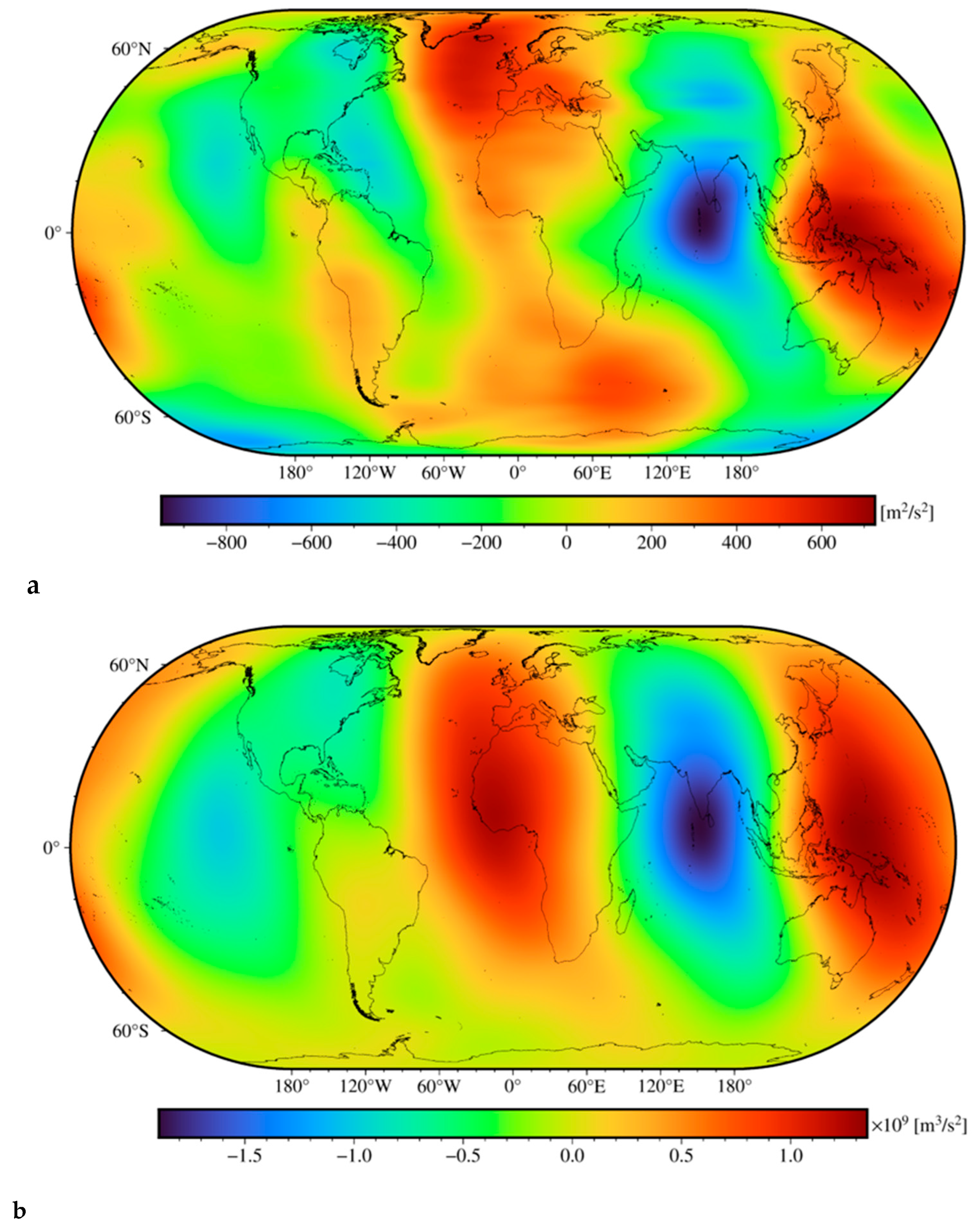
As seen in Equation (17), the values of the radially integrated disturbing potential are computed in spectral form from the spherical harmonics $T_{n,m}$ of disturbing potential scaled by the factor 1/n. This scaling factor lessens the contribution of higher-degree spherical harmonics so that their combined contribution in the radial integral of Earth’s disturbing potential becomes significantly smaller than that of the Earth’s disturbing potential. The smoothing effect is demonstrated in Figure 1, where we plotted the Earth’s disturbing potential and its radial integral, both computed globally on a 1 arc-deg equiangular grid from the EIGEN-6C4 coefficients up to degree n = 180. A spatial pattern and spectrum of the radial integral of the disturbing potential were investigated and compared with other parameters of the gravity field in [24]. They acquired that this smoothing is explained by the fact that more detailed features in the disturbing potential (mainly attributed to a gravitational signature of lithospheric density structure and geometry) are filtered out proportionally with increasing degree of spherical harmonics in this functional.

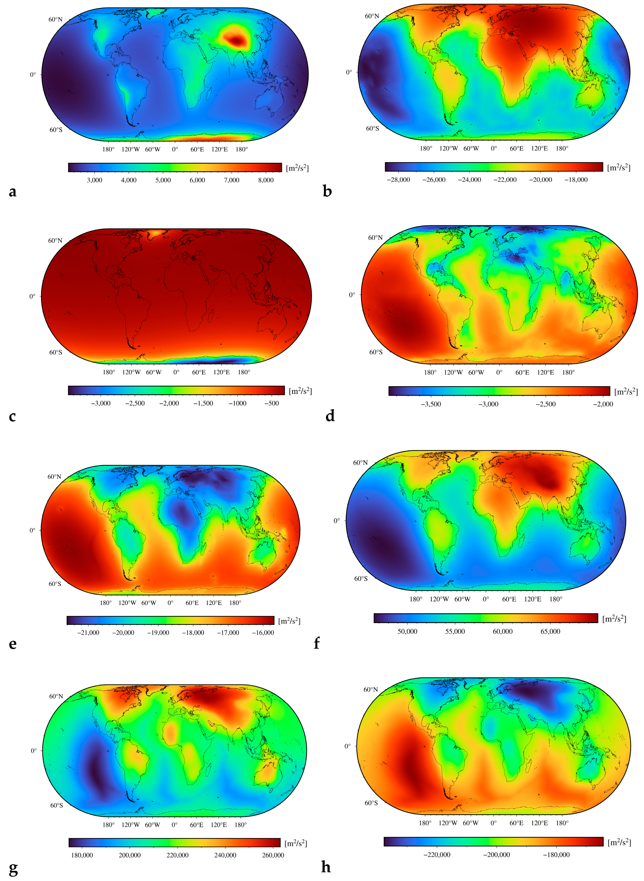
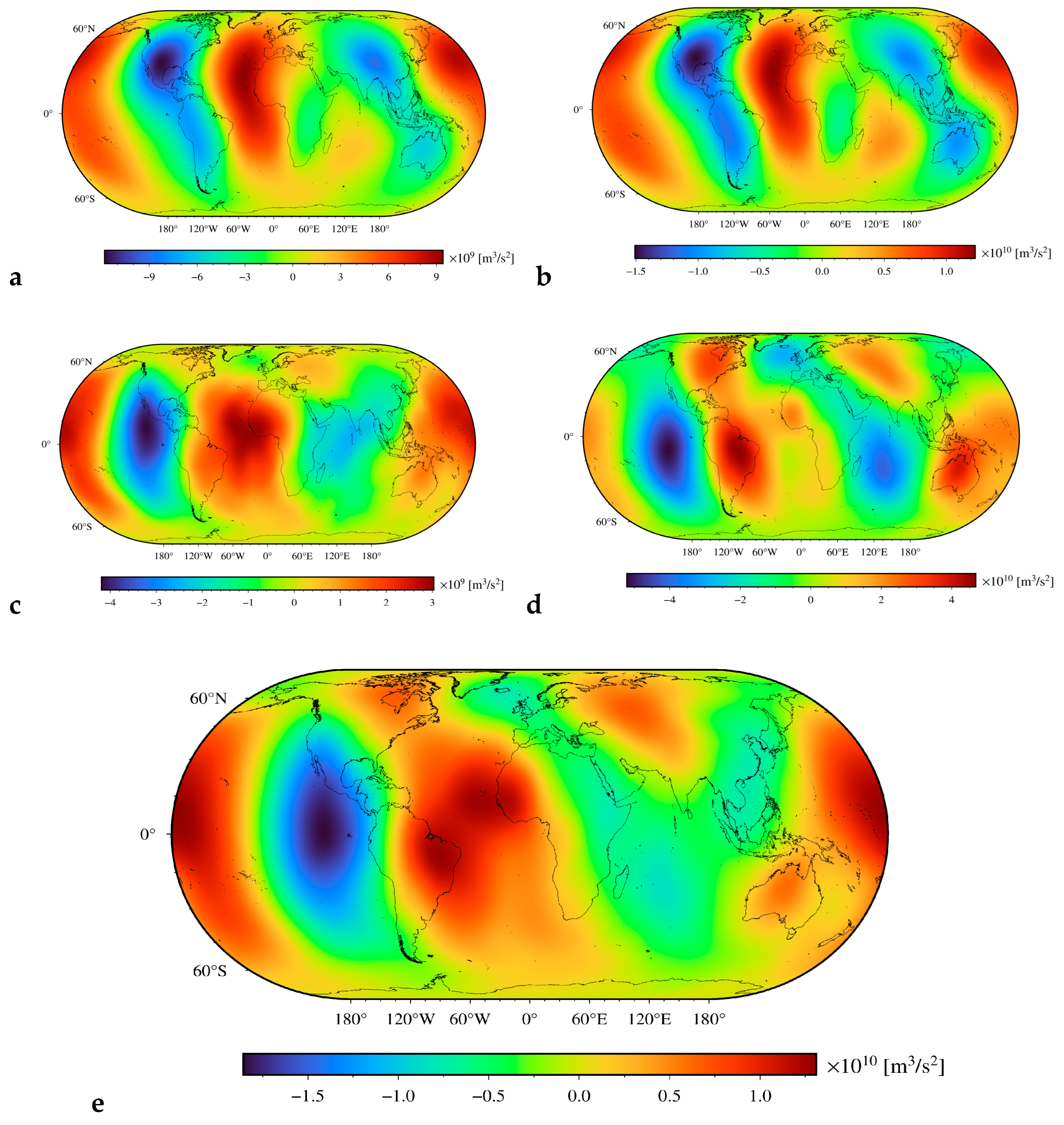
We further inspected the possibility of enhancing the signature of the deep mantle by subtracting the gravitational contribution of the lithospheric geometry and density structure from the Earth’s disturbing potential and its radial integral. Results are presented in Figure 2, Figure 3, Figure 4 and Figure 5, with statistical summaries of results in

Table 1. The statistics of gravitational potentials of lithospheric geometry and density structure components used to compute the sub-lithospheric mantle disturbing potential. For notation used, see legend in Figure 2.

Gravitational Potential	Min [m2 s−2]	Max [m2 s−2]	Mean [m2 s−2]	STD [m2 s−2]
$V^T$	2226	8494	3589	1114
$V^B$	−28,533	−16,402	−22,386	3185
$V^I$	−3472	−312	−731	729
$V^S$	−10,405	−6051	−8207	977
$V^C$	−25,077	−11,529	−15,661	2741
$V^{M,\Delta {\rho }^{c,m}}$	46,423	69,885	55,734	5832
$V^{LM}$	174,276	262,661	213,366	17,795
$V^{LAB}$	−244,558	−168,987	−203,311	16,194

,

Table 2. Statistics of disturbing potentials. For notation used, see legend in Figure 3.

Disturbing Potential	Min [m2 s−2]	Max [m2 s−2]	Mean [m2 s−2]	STD [m2 s−2]
$T$	−1036	833	−8	284
$T^B$	9002	26,971	19,657	3858
$T^{CS}$	−14,811	9079	−1369	5769
$T^M$	52,335	57,176	54,455	954
$T^{CL}$	228,091	319,453	268,166	18,230
$T^{SM}$	62,079	81,743	70,517	3649

,

Table 3. The statistics of the radially integrated potentials presented in Figure 4, used to compute the radial integral of the sub-lithospheric mantle disturbing potential.

Radially Integrated Gravitational Potential	Min [m3 s−2]	Max [m3 s−2]	Mean [m3 s−2]	STD [m3 s−2]
${\displaystyle \underset{r}{\int }{V}^T \mathrm{d}r}$	−2.3878 × 109	3.8872 × 109	−1.6962 × 10−9	8.2504 × 108
${\displaystyle \underset{r}{\int }{V}^B \mathrm{d}r}$	−6.7750 × 109	8.5480 × 109	−3.6462 × 10−9	2.7199 × 109
${\displaystyle \underset{r}{\int }{V}^I \mathrm{d}r}$	−2.8656 × 108	2.9741 × 108	−1.3294 × 10−10	5.5653 × 107
${\displaystyle \underset{r}{\int }{V}^S \mathrm{d}r}$	−9.7560 × 108	5.5993 × 108	−1.2702	2.7608 × 108
${\displaystyle \underset{r}{\int }{V}^C \mathrm{d}r}$	−3.6042 × 109	2.6121 × 109	48.9703	1.1868 × 109
${\displaystyle \underset{r}{\int }{V}^{M,\Delta {\rho }^{c/m}} \mathrm{d}r}$	−1.0518 × 1010	1.3199 × 1010	1.0145 × 10−8	4.3710 × 109
${\displaystyle \underset{r}{\int }{V}^{LM} \mathrm{d}r}$	−4.8607 × 1010	4.5146 × 1010	−1.8737 × 10−8	1.5163 × 1010
${\displaystyle \underset{r}{\int }{V}^{LAB} \mathrm{d}r}$	−2.3878 × 109	3.8872 × 109	−1.6962 × 10−9	8.2504 × 108

and

Table 4. Statistics of the radially integrated disturbing potentials presented in Figure 5.

Radially Integrated Disturbing Potential	Min [m3 s−2]	Max [m3 s−2]	Mean [m3 s−2]	STD [m3 s−2]
${\displaystyle \underset{r}{\int }T \mathrm{d}r}$	−1036	833	−8	284
${\displaystyle \underset{r}{\int }{T}^B \mathrm{d}r}$	−1.1818 × 1010	9.4317 × 109	−119.97	3.6716 × 109
${\displaystyle \underset{r}{\int }{T}^{CS} \mathrm{d}r}$	−1.5103 × 1010	1.2340 × 1010	−76.70	4.8540 × 109
${\displaystyle \underset{r}{\int }{T}^M \mathrm{d}r}$	−4.1926 × 109	3.0366 × 109	−274.68	1.2042 × 109
${\displaystyle \underset{r}{\int }{T}^{CL} \mathrm{d}r}$	−5.2214 × 1010	4.6829 × 1010	−2894.21	1.5935 × 1010
${\displaystyle \underset{r}{\int }{T}^{SM} \mathrm{d}r}$	−1.8577 × 1010	1.3109 × 1010	−3182.16	5.3405 × 109

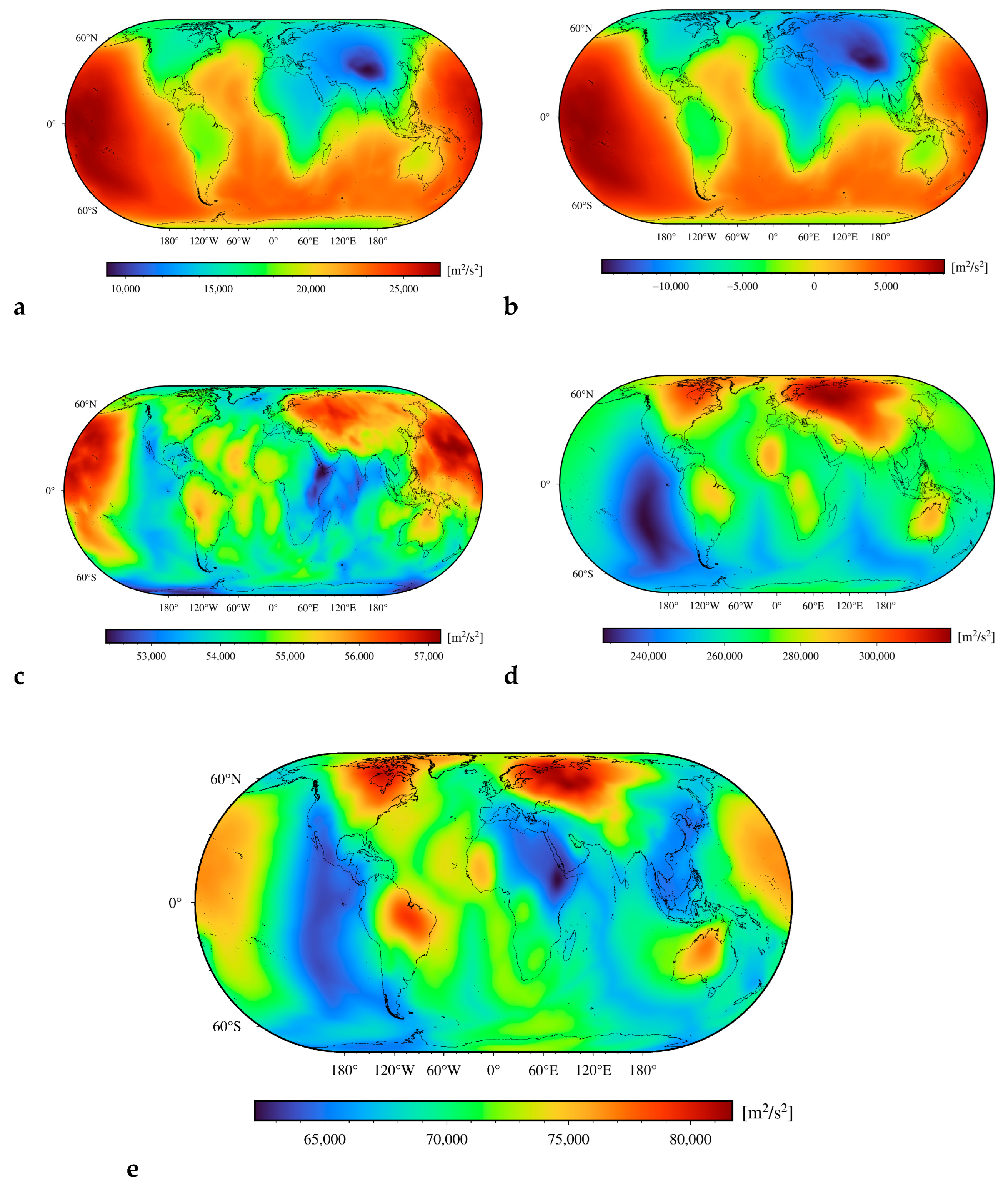
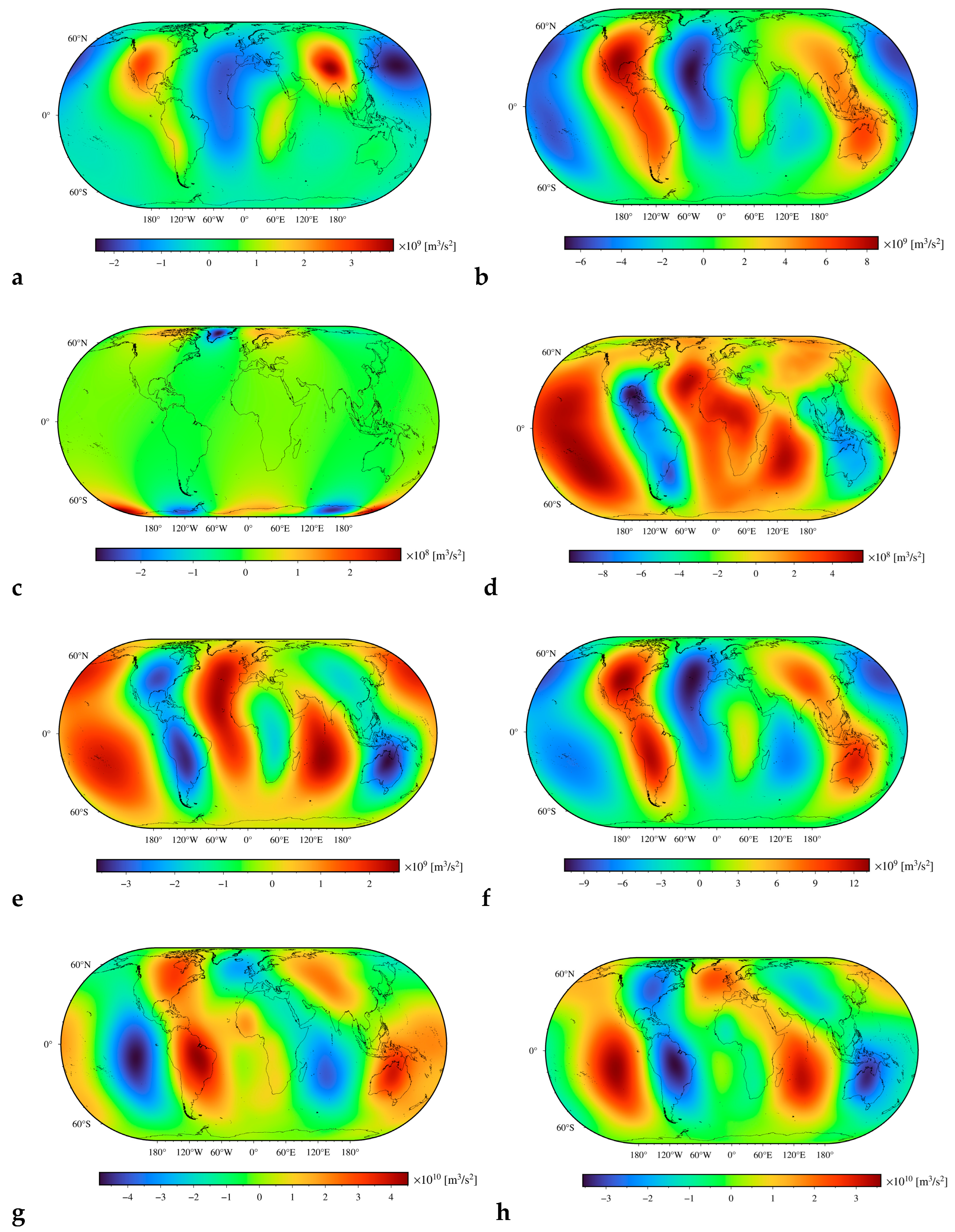
. In Figure 2, we plotted the gravitational potentials of lithospheric density and geometry structure components subtracted from the Earth’s disturbing potential to obtain the sub-lithospheric mantle disturbing potential. The intermediate results after subtracting individual gravitational contributions and the final solution, i.e., the sub-lithospheric mantle disturbing potential, are plotted in Figure 3. The corresponding corrections and results for the radially integrated values are shown in Figure 4 and Figure 5, respectively.

5. Discussion

The Earth’s topography is primarily controlled by the lateral density variations within the lithosphere as well as tectonic motions and lithospheric stresses, while global mantle flow induces deformations of its surface, leading to dynamic topography. As seen in Figure 6, where we plotted the dynamic topography model prepared by Rubey et al. [36], the deep mantle structure is dominated by two large antipodal low shear-velocity provinces at the base of the mantle (e.g., [5]). More detailed features involve large negative anomalies along active convergent margins, including oceanic subductions and continental collisions. It is worth noting that dynamic topography models prepared by other authors generally exhibit a pattern that is similar to that seen in Figure 6. A similar pattern is apparent in the Earth’s disturbing potential. As seen in Figure 1a, the Earth’s disturbing potential is manifested by two large positive anomalies that are coupled by large negative anomalies attributed to mantle downwelling in mantle convection. A similar pattern is seen in the radially integrated disturbing potential (see Figure 1b), with more detailed features attributed to the lithospheric density structure filtered out after applying the integral operator. Consequently, the radially integrated disturbing potential is more suitable to interpret the deep mantle than the disturbing potential (or the geoid).

We further compared the dynamic topography model, shown in Figure 6, with the results obtained after removing the gravitational contribution of the lithospheric geometry and density structure (including the LAB geometry) from the Earth’s disturbing potential and its radial integral. As seen in Figure 3e and Figure 5e, the sub-lithospheric mantle disturbing potential and its radial integral more closely replicate the dynamic topography than the Earth’s disturbing potential and its radial integral. Nevertheless, we also observe some significant discrepancies between the dynamic topography and our two results (i.e., the sub-lithospheric mantle disturbing potential and its radial integral). The negative anomaly in the dynamic topography along America is systematically shifted westwards in both refined results, and with a similar systematic shift of the positive anomaly over Africa. The margins of the Pacific positive anomaly, on the other hand, coincide quite closely in the West Pacific, but completely disagree over Australia, where the dynamic topography reaches minimum values, while values in both refined results there reach local maxima.

As seen in Figure 3e, the lithospheric signature is still strongly manifested in the sub-lithospheric mantle disturbing potential, particularly along active divergent tectonic margins, while this pattern is filtered out in the radially integrated sub-lithospheric mantle disturbing potential (see Figure 5e). Consequently, the application of the integral operator to disturbing potential and mathematical removal of the respective gravitational contribution of the lithospheric geometry and density structure provides the result that most closely agrees with the dynamic topography and appears the most suitable for gravimetric interpretation of lateral density distribution within the deep mantle.

The results presented in this study depend on the accuracy of global gravitational and lithospheric density models used for numerical realization. The errors in the computed values of the disturbing potential and its radial integral due to uncertainties of the global gravitational model (EIGEN-6C4) are negligible when compared to much larger errors attributed to uncertainties of lithospheric density models (CRUST1.0, LITHO1.0). The uncertainties of both lithospheric density models were assessed in [37]. According to their estimates, relative errors up to 10–20% could be expected in results presented through Figure 2, Figure 3, Figure 4 and Figure 5, given that errors in the density values propagate almost proportionally to errors in the computed gravity field quantities. Moreover, the errors typically increase with depth due to increasing uncertainties of estimated rock densities from tomographic surveys. It is important to note that despite several functional relations between rock density and seismic velocities that have been developed based on the analysis of tomographic data while incorporating geophysical, geochemical, and geothermal constraints, these density models might be widely inaccurate due to several reasons. A major limiting factor is insufficient coverage in many parts of the world by tomographic surveys. The refinement of 1D reference density models by incorporating 2D or 3D lithospheric density models is then complicated. Furthermore, the direct relation between seismic velocities and mass densities does not exist because density distribution depends on many other factors (such as temperature, mineral composition, and pressure).

6. Summary and Concluding Remarks

We have investigated the possibility of interpreting lateral density distribution within the deep mantle by applying the integral operator to the disturbing potential. In the definition of the radially integrated disturbing potential, spherical harmonics of the disturbing potential are scaled by the factor $1/n$, thus reducing the contribution of higher-degree spherical harmonic terms. Consequently, the radially integrated disturbing potential better enhances the long-wavelength signature of the deep mantle than the disturbing potential. This integral operator can then be used as an effective filtering technique together with the spherical harmonic decomposition. In other words, the scaling factor $1/n$ is first applied to spherical harmonic terms of the disturbing potential, for $n>0$. Note that the radial integral of the zero-degree term $GM/r$ is a ln function. The spherical harmonic decomposition can then be applied to select a maximum degree of spherical harmonics of the radially integrated disturbing potential used for the gravimetric interpretation of the deep mantle.

We further investigated the possibility of enhancing the signature of the deep mantle by subtracting the gravitational contribution of lithospheric geometry and density structure from the disturbing potential and its radial integral. Both results (i.e., the sub-lithospheric mantle disturbing potential and its radial integral) exhibited better agreement with the dynamic topography model than the corresponding results before applying this refinement (i.e., the disturbing potential and its radial integral). Nevertheless, our numerical findings indicate that the radially integrated sub-lithospheric mantle disturbing potential is the most suitable for gravimetric interpretation of lateral density variations within the deep mantle. The main reason is that the sub-lithospheric mantle disturbing potential still comprises the gravitational signature of the lithosphere, particularly along active divergent tectonic margins, while this pattern was completely filtered out in its radially integrated solution.

Summarizing our numerical findings, we argue that the application of the integral operator to disturbing potential generally improves the gravimetric interpretation of the deep mantle by filtering out the gravitational contribution of higher-degree spherical harmonic terms, mainly attributed to the lithospheric geometry and density structure. Nevertheless, this mathematical operation alone cannot fully remove the gravitational contribution of the lithosphere because it occupies the whole gravity spectrum with its largest contribution at low-degree spherical harmonics. The gravimetric forward modeling should be applied to model and completely remove the gravitational contribution of the lithospheric geometry and density structure. Consequently, the combined application of the integral operator and forward modelling provides the best result for the gravimetric interpretation of lateral density variations within the deep mantle in terms of the radially integrated sub-lithospheric mantle disturbing potential. This result agrees most closely with the spatial pattern of dynamic topography. The sub-lithospheric mantle disturbing potential, on the other hand, still comprises the lithospheric signature, with a redundant pattern that closely resembles the LAB geometry as well as a thermal signature that significantly controls density variations, particularly within the lithospheric mantle. This redundant lithospheric signature is likely due to large errors in the LITHO1.0 and CRUST1.0 datasets of lithospheric mantle density and thickness. These errors are partially filtered out after applying the integral operator. However, it is important to emphasize that large-scale errors in lithospheric models remain even after applying the integral operator, especially at low-degree spherical harmonic terms that cannot be filtered out.

References

- Hager, B.H.; Clayton, R.W.; Richards, M.A.; Comer, R.P.; Dziewonski, A.M. Lower mantle heterogeneity, dynamic topography and the geoid. Nature 1985, 313, 541–545. [Google Scholar] [CrossRef]
- Hager, B.; Richards, M. Long-wavelength variations in Earth’s geoid: Physical models and dynamical implications. Philos. Trans. R. Soc. Math. Phys. Sci. 1989, 328, 309–327. [Google Scholar] [CrossRef]
- Wen, L.; Anderson, D.L. Layered mantle convection: A model for geoid and topography. Earth Planet. Sci. Lett. 1997, 146, 367–377. [Google Scholar] [CrossRef]
- Zhong, S.; Davies, G. Effects of plate and slab viscosities on the geoid. Earth Planet. Sci. Lett. 1999, 170, 487–496. [Google Scholar] [CrossRef]
- Steinberger, B. Slabs in the lower mantle—Results of dynamic modelling compared with tomographic images and the geoid. Phys. Earth Planet. Inter. 2000, 118, 241–257. [Google Scholar] [CrossRef]
- Zhong, S. Role of ocean-continent contrast and continental keels on plate motion, net rotation of lithosphere and the geoid. J. Geophys. Res. 2001, 106, 703–712. [Google Scholar] [CrossRef]
- Čadek, O.; Fleitout, L. Effect of lateral viscosity variations in the top 300 km on the geoid and dynamic topography. Geophys. J. Int. 2003, 152, 566–580. [Google Scholar] [CrossRef]
- Moucha, R.; Forte, A.; Mitrovica, J.; Daradich, A.D. Lateral variations in mantle rheology: Implications for convection related surface observables and inferred viscosity models. Geophys. J. Int. 2007, 169, 113–135. [Google Scholar] [CrossRef]
- Yoshida, M.; Nakakuki, T. Effects on the long-wavelength geoid anomaly of lateral viscosity variations caused by stiff subducting slabs, weak plate margins and lower mantle rheology. Phys. Earth Planet. Inter. 2009, 172, 278–288. [Google Scholar] [CrossRef]
- Ghosh, A.; Becker, T.W.; Zhong, S.J. Effect of lateral viscosity variations on the geoid. Geophys. Res. Lett. 2010, 37, L01301. [Google Scholar] [CrossRef]
- Coblentz, D.; van Wijk, J.; Richardson, R.M.; Sandiford, M. The upper mantle geoid: Implications for continental structure and the intraplate stress field. In The Interdisciplinary Earth: A Volume in Honor of Don L. Anderson; Foulger, G.R., Lustrino, M., King, S.D., Eds.; Special Paper 514; Geological Society of America: Boulder, CO, USA, 2015. [Google Scholar] [CrossRef]
- Sandwell, D.T.; Müller, R.D.; Smith, W.H.F.; Garcia, E.; Francis, R. New global marine gravity model from CryoSat-2 and Jason-1 reveals buried tectonic structure. Science 2014, 346, 65–67. [Google Scholar] [CrossRef] [PubMed]
- Braitenberg, C.; Wienecke, S.; Wang, Y. Basement structures from satellite-derived gravity field: South China Sea ridge. J. Geophys. Res. 2006, 111, B05407. [Google Scholar] [CrossRef]
- Shin, Y.H.; Xu, H.; Braitenberg, C.; Fang, J.; Wang, Y. Moho undulations beneath Tibet from GRACE-integrated gravity data. Geophys. J. Int. 2007, 170, 971–985. [Google Scholar] [CrossRef]
- Braitenberg, C.; Ebbing, J. New insights into the basement structure of the west-Siberian basin from forward and inverse modelling of Grace satellite gravity data. J. Geophys. Res. 2009, 114, B06402. [Google Scholar] [CrossRef]
- Alvarez, O.; Gimenez, M.; Braitenberg, C.; Folguera, A. GOCE Satellite derived Gravity and Gravity gradient corrected for topographic effect in the South Central Andes Region. Geophys. J. Int. 2012, 190, 941–959. [Google Scholar] [CrossRef]
- Mahatsente, R.; Önal, G.; Çemen, I. Lithospheric structure and the isostatic state of Eastern Anatolia: Insight from gravity data modelling. Lithosphere 2018, 10, 279–290. [Google Scholar] [CrossRef]
- Chisenga, C.; Yan, J. A new crustal thickness model for mainland China derived from EIGEN-6C4 gravity data. J. Asian Earth Sci. 2019, 179, 430–442. [Google Scholar] [CrossRef]
- Rathnayake, S.; Tenzer, R.; Eshagh, M.; Pitoňák, M. Gravity maps of the lithospheric structure beneath the Indian Ocean. Surv. Geophys. 2019, 40, 1055–1093. [Google Scholar] [CrossRef]
- Tenzer, R.; Bagherbandi, M.; Chen, W.; Sjöberg, L.E. Global isostatic gravity maps from satellite missions and their applications in the lithospheric structure studies. IEEE J. Sel. Top. Appl. Earth Obs. Remote Sens. 2016, 10, 549–561. [Google Scholar] [CrossRef]
- Laske, G.; Masters, G.; Ma, Z.; Pasyanos, M.E. Update on CRUST1.0—A 1-degree global model of Earth’s crust. Geophys. Res. Abstr. 2013, 15, EGU2013-2658. [Google Scholar]
- Pasyanos, M.E.; Masters, T.G.; Laske, G.; Ma, Z. LITHO1.0: An updated crust and lithospheric model of the Earth. J. Geophys. Res. 2014, 119, 2153–2173. [Google Scholar] [CrossRef]
- Tenzer, R.; Chen, W. Mantle and sub-lithosphere mantle gravity maps from the LITHO1.0 global lithospheric model. Earth-Sci. Rev. 2019, 194, 38–56. [Google Scholar] [CrossRef]
- Tenzer, R.; Novák, P.; Eshagh, M. The radial integral of the geopotential. Surv. Geophys. 2025. [Google Scholar] [CrossRef]
- Heiskanen, W.; Moritz, H. Physical Geodesy; WH Freeman and Co.: San Francisco, CA, USA; London, UK, 1967. [Google Scholar]
- Förste, C.; Bruinsma, S.L.; Abrikosov, O.; Lemoine, J.M.; Marty, J.C.; Flechtner, F.; Balmino, G.; Barthelmes, F.; Biancale, R. EIGEN-6C4 The latest combined global gravity field model including GOCE data up to degree and order 2190 of GFZ Potsdam and GRGS Toulouse. In Proceedings of the 5th GOCE User Workshop, Paris, France, 25–28 November 2014. [Google Scholar] [CrossRef]
- Hirt, C.; Rexer, M. Earth2014: 1 arc-min shape, topography, bedrock and ice-sheet models—Available as gridded data and degree-10,800 spherical harmonics. Int. J. Appl. Earth Obs. Geoinf. 2015, 39, 103–112. [Google Scholar] [CrossRef]
- Sheng, M.B.; Shaw, C.; Vaníček, P.; Kingdon, R.W.; Santos, M.; Foroughi, I. Formulation and validation of a global laterally varying topographical density model. Tectonophysics 2019, 762, 45–60. [Google Scholar] [CrossRef]
- Divins, D.L. Total Sediment Thickness of the World’s Oceans and Marginal Seas; NOAA Natl Geophys Data Cent: Boulder, CO, USA, 2003. [Google Scholar]
- Moritz, H. Geodetic Reference System 1980. J. Geod. 2000, 74, 128–133. [Google Scholar] [CrossRef]
- Hinze, W.J. Bouguer reduction density, why 2.67? Geophys. 2003, 68, 1559–1560. [Google Scholar] [CrossRef]
- Artemjev, M.E.; Kaban, M.K.; Kucherinenko, V.A.; Demjanov, G.V.; Taranov, V.A. Subcrustal density inhomogeneities of northern Eurasia as derived from the gravity data and isostatic models of the lithosphere. Tectonophysics 1994, 240, 248–280. [Google Scholar] [CrossRef]
- Cutnell, J.D.; Kenneth, W.J. Physics, 3rd ed.; Wiley: New York, NY, USA, 1995. [Google Scholar]
- Gladkikh, V.; Tenzer, R. A mathematical model of the global ocean saltwater density distribution. Pure Appl. Geophys. 2012, 169, 249–257. [Google Scholar] [CrossRef]
- Baranov, A.; Tenzer, R.; Bagherbandi, M. Combined gravimetric-seismic crustal model for Antarctica. Surv. Geophys. 2018, 39, 23–56. [Google Scholar] [CrossRef]
- Rubey, M.; Brune, S.; Heine, C.; Davies, D.R.; Williams, S.E.; Müller, R.D. Global patterns of Earth’s dynamic topography since the Jurassic: The role of subducted slabs. Solid. Earth 2017, 8, 899–919. [Google Scholar] [CrossRef]
- Tenzer, R.; Chen, W. The accuracy assessment of lithospheric density models. Appl. Sci. 2023, 13, 10432. [Google Scholar] [CrossRef]