Abstract
In this study, we analyzed the microearthquake seismicity in the Enguri area (Georgia) recorded between 2020 and 2023 using a newly installed seismic network developed within the DAMAST project. The high sensitivity of the network allowed the detection of even very small seismic events, enabling a detailed investigation of the temporal dynamics of local seismicity. Statistical analyses suggest that the seismic activity around the Enguri Dam is influenced by a combination of natural tectonic processes and subtle reservoir-induced stress changes. While the dam does not appear to exert strong seismic forcing, the observed ≈7-month delay between water level variations and seismicity may indicate a triggering effect. Localized stress variations and temporal clustering further support the hypothesis that water level fluctuations modulate seismic activity. Additionally, the mild persistence in interoccurrence times is consistent with a stress accumulation and delayed triggering mechanism associated with reservoir loading.
1. Introduction
The Enguri Dam is situated along the Enguri River, which flows through the northwest part of Georgian territories, including the region of Abkhazia, and plays a crucial role in the country’s power supply. It is situated in the northwestern part of Georgia, within the southern section of the Greater Caucasus Mountains, where the ongoing convergence between the Eurasian and African–Arabian plates results in folding, thrusting, and crustal shortening [1,2,3,4,5]. Previous studies have extensively examined the seismotectonic characteristics of the Enguri area, including GPS-derived convergence rates [1,6,7,8,9,10], regional fault systems [11,12,13], and seismicity patterns [14,15].
Standing at 271 m, the Enguri Dam is among the tallest arch dams in the world. Its reservoir, with an mean volume of 1 billion cubic meters and yearly water level fluctuations of approximately 100 m, is situated in close proximity to active faults. This unique setting makes it a compelling case study for reservoir-triggered seismicity and the complex interactions between dam reservoirs and fault systems [16]. According to Basili et al. [17], the active fault structures around the Enguri Dam pose the most significant seismic hazard to the Enguri Hydropower Plant (HPP).
In the framework of the DAMAST (Dams and Induced Seismicity Transfer for Sustainability) project (https://www.damast-caucasus.de/68.php), a local modern seismic network was installed to monitor the seismic activity around the Enguri Dam. The newly established local seismic network consists of four surface stations, three stations located in shallow boreholes and one in a deep borehole. Such significant advancements in the local seismic network, developed within the DAMAST project, enhanced the detection capabilities, allowing even minor seismic events to be recorded. This improvement enables a more detailed examination of the catalog’s properties. Although the recorded seismicity shows activity along existing faults, ongoing studies are focused on the detailed identification of active fault branches, their geometry, and slip mechanisms, as well as exploring the potential connection between seismic activity and fluctuations in the dam-reservoir water levels.
In this work, we aim to provide a comprehensive statistical analysis of the temporal and magnitude distribution characteristics of the seismicity of the Enguri area recorded from 2020 to 2023 within the DAMAST project. In addition to well-established seismological and statistical metrics—such as the b-value of the Gutenberg–Richter law, the magnitude of completeness, and the coefficient of variation (both global and local)—this study examines the clustering in the time distribution of the Enguri seismicity by using the Allan factor analysis, as well as the correlation properties of the interevent times and magnitude by means of the detrended fluctuation analysis, and, moreover, introduces a novel set of parameters to characterize the seismicity of the region under study. These parameters are derived from the visibility graph (VG) method, originally developed by Lacasa et al. [18], and then increasingly utilized in recent studies to analyze seismic sequences [19,20].
Our study focuses also on the correlation between the seismicity and water level of the Enguri Dam. Information on water level fluctuations at the Enguri reservoir was obtained in collaboration with LTD Engurhesi, the operator of the Enguri Hydropower Plant (HPP) [21]. The dataset consists of daily reservoir elevation records, systematically collected since the dam’s commissioning in the 1970s and continuously maintained to the present. For this study, we focused on the 2020–2023 period to facilitate comparison with the local seismicity catalog [22].
2. Seismo-Tectonic Settings
The Enguri Dam is located directly on the Mukhuri segment (MS) of the reverse Racha-Lechkhumi fault system, which extends with a strike of 288°. The average (mean) maximum magnitude for this fault is estimated at 6.61, with a mean slip rate of 0.375 mm/year. The largest historical earthquake, the Kvira event (Mw = 6.9; 1250), occurred along this fault. The magnitude of this earthquake corresponds closely to the 98th percentile estimate of the maximum magnitude (MWMAXP98 = 6.92) for the Mukhuri segment, meaning there is only a 2% probability that the actual maximum magnitude exceeds this value. To the south, the Enguri Dam area is surrounded by three segments of the Odishi active fault system. The Achigvara (OA) segment (strike 350°) and the Martvili (OM) segment (strike 233°) represent right-lateral and left-lateral faults, respectively, while the Khobi (OKH)segment (strike 298°) is characterized as a reverse fault. The Odishi fault has an average maximum magnitude of 6.43 and a slip rate of 0.1 mm/year. At the junction of the Achigvara and Khobi faults, a historical earthquake with Mw = 6.1 occurred in the year 1614. Another active fault that could significantly impact the Enguri HPP is the Larakvakva reverse fault, which consists of two branches—North and South—crossing the Jvari Reservoir. The Larakvakva South branch (LS) has a strike of 288° and an average maximum magnitude (Mwmax) of 6.61. A historical earthquake, the 1750 Akiba event (Mw = 7.0), occurred along this fault. The magnitude of this earthquake closely corresponds to the 98th percentile estimate of the maximum magnitude (MWMAXP98 = 7.02). The average slip rate of the fault is 0.17 mm/year, with the North branch (LN) being more active, exhibiting an average Mw of 6.74 and a slip rate of 0.34 mm/year.
Figure 1 presents the surface projection of active faults around the Enguri Dam [17], along with the investigated seismicity (yellow dots) recorded by the new local seismic network developed within the DAMAST project within 33 km radius around the Enguri Dam and down to 30 km depth. The dataset covers the period from 1 October 2020 to 31 December 2023, and the earthquake magnitudes range from −1.3 to 3.3. Seismic activity is notably high along the Mukhuri segment, affecting both branches of the Larakvakva reverse fault and the Achigvara segment. Additionally, significant seismicity is observed along the pressure tunnel that connects the Jvari reservoir to the powerhouse at the Gali Reservoir (Abkhazia), located approximately 15 km southwest of the Enguri High Dam. Old literature published by Murusidze in 1980 [23] references the so-called ‘Enguri faults,’ marked by red dashed lines in Figure 1, which are clearly visible in the topography. However, these faults are not included in the European active fault database [17], primarily due to insufficient investigation. Based on the seismic activity pattern, we can infer that the Ingrishi faults are quite active and may extend farther southwest toward the Gali Reservoir (GR).
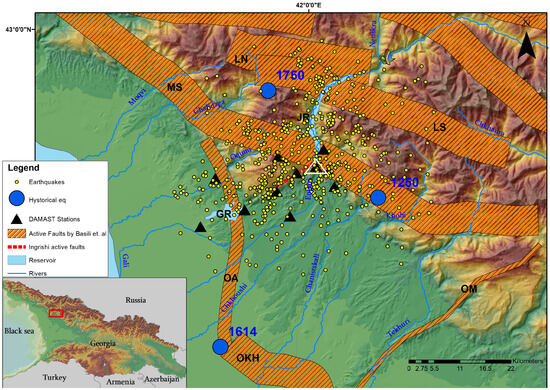
Figure 1.
Seismicity and active fault structures in the Enguri Dam region. Yellow circles indicate microearthquakes recorded between 2020 and 2023; large blue circles mark historical earthquakes. DAMAST seismic stations are shown as black triangles. Active faults from Basili et al. [17] (hatched areas) and locally identified Ingrishi fault segments (red dashed lines) are overlaid. Major rivers, the Jvari Reservoir (JR), Gali Reservoir (GR), and the location of the Enguri Dam (white triangle) are labeled. Inset: Regional map showing the location of the study area (red box) within Georgia and surrounding countries.
3. Seismic Network and Data
3.1. Description of the Seismic Network
A ten-station local seismic network was established to monitor low-magnitude seismic activity near the Enguri Dam. Seven of the stations are located within a 10 km radius of the dam, while the remaining three are within a 10 km radius of the Gali Reservoir, ensuring comprehensive coverage with enhanced sensitivity near active fault segments, as illustrated in Figure 1.
In this study, we used a dedicated seismic catalog independently constructed from continuous waveform data recorded by the local seismic network deployed around the Enguri Dam within the DAMAST project. This catalog was not derived from any official or national database. The network, specifically designed to monitor microseismicity near the dam, enables the detection of events with magnitudes well below the threshold of the national seismic monitoring system [15].
The finalized configuration of the deployed network around the Enguri Dam, comprising both surface and borehole stations, includes Centaur data loggers, routers, and SIM cards for data transmission at each active station. The network was deployed in five major phases: October 2020, December 2020, September 2021, January 2022, and October 2023. The initial deployment consisted of five stations, followed by the addition of two more. Subsequently, one station was installed in the Abkhazia region, with two additional stations added later. The coordinates and elevations of these stations are provided in Table 1.

Table 1.
Coordinates and elevations of seismic stations.
Among the stations, KIT1 and HPP are powered by AC electricity, while the others rely on solar panels combined with battery storage. Most stations (KIT1, NIKA, BUFF, BRID, KETI, and DOG) have maintained continuous data recording and transmission since their installation. Site selection was significantly influenced by challenging terrain on the western side of the dam reservoir and restrictions near the Georgia–Abkhazia border. Despite these obstacles, the GULB station was successfully installed in a high-altitude mountainous area. However, due to unreliable real-time data transmission and extremely difficult—sometimes impossible—access, the GULB station was decommissioned in June 2023.
Borehole stations are equipped with Isometrics Trillium Compact Posthole 20s (TC20PH2) broadband sensors installed at depths of 17–20 m (BUFF: 19 m, NIKA: 17 m, DOG: 20 m) and 250 m (KIT1), effectively minimizing surface noise. These sensors provide a flat velocity response over a broad frequency range, from approximately 0.008 Hz to beyond 100 Hz, in accordance with manufacturer specifications and confirmed by instrument response spectra analysis. Their self-noise levels approach the New Low Noise Model (NLNM) within the most sensitive portion of the seismic band, making them ideal for low-noise borehole environments. Additionally, they offer a dynamic range exceeding 156 dB at 1 Hz. Data acquisition is handled by Centaur CTR4-3 digitizers, which deliver 24-bit resolution, GPS-based timing, and onboard data storage.
Surface broadband stations (KETI, BRID, and GULB) are equipped with Kinemetrics MBB-2 sensors connected to Centaur digitizers. These sensors exhibit a flat velocity response between approximately 0.03 Hz and 80 Hz, as confirmed by pole-zero analysis. Although they are nominally specified down to 0.0083 Hz (120 s), the effective usable bandwidth is more limited in practice. Their dynamic range exceeds 155 dB at 1 Hz, and careful mechanical coupling during field installation helps minimize noise.
Short-period installations (e.g., OKM, HPP, and GAL), especially in remote or access-restricted areas, employ three-component 4.5 Hz geophones (type PE-6/B) connected to compact DATA-CUBE3 Type 2 recorders. These sensors provide a flat velocity response above 4.5 Hz, with a usable bandwidth extending up to 80 Hz. The geophone response spectra were modeled using simplified empirical two-pole transfer functions, validated through SEED RESP files. This configuration offers a dynamic range of approximately 100–110 dB, ensuring high sensitivity for detecting shallow microseismic events.
The instrument responses at all stations were verified using SEED RESP files, ensuring consistent response spectra across each component (HHE, HHN, and HHZ) of the same sensor model. These responses include the complete pole-zero structure, gain, and normalization factors, and were uniformly applied during data correction and processing. A summary is provided in Table 2.
Table 2.
Instrument response characteristics by sensor type and station class.
3.2. Seismic Ambient Noise Analysis and Station Performance
To evaluate the ambient noise environment at each seismic station, we analyzed the root-mean-square (Vrms) velocity amplitudes of both vertical and horizontal components by integrating the power spectral density (PSD). Two frequency bands were selected to characterize the noise: 1–10 Hz, which captures the dominant energy of local and regional events and is critical for local magnitude () estimation, and 5–15 Hz, which highlights high-frequency noise that may impact the detectability of small-magnitude () events.
The Vrms values (see Table 3) exhibit considerable variability across the network. Borehole stations—including KIT1 and the shallower boreholes BUFF, NIKA, and DOG—consistently show the lowest Vrms levels, confirming their superior performance for microseismic monitoring and reliable magnitude calibration.
Table 3.
Root-mean-square (Vrms) velocity amplitudes across vertical and horizontal components in two frequency bands (1–10 Hz and 5–15 Hz) for all stations in the Enguri seismic network.
The surface broadband station GULB, located in a high-altitude alpine environment, also demonstrated excellent noise performance prior to its removal in mid-2023, providing valuable high-quality data during its operational period. In contrast, surface stations such as KETI and GAL exhibit elevated Vrms levels, with GAL particularly noisy in the 5–15 Hz band—likely due to local anthropogenic activity or wind-induced noise. The OKM and HPP stations show intermediate noise levels, likely benefiting from more favorable site conditions.
To further evaluate station performance, we calculated the median vertical-component power spectral density (PPSD) [24] for each station using the ObsPy PPSD module. The resulting spectra were plotted against the New High Noise Model (NHNM) and New Low Noise Model (NLNM) [25] defined by Peterson (1993) [26], which serve as the global reference standards for seismic noise levels (Figure 2). PPSD values are reported in decibels (dB) relative to , representing acceleration power spectral density.
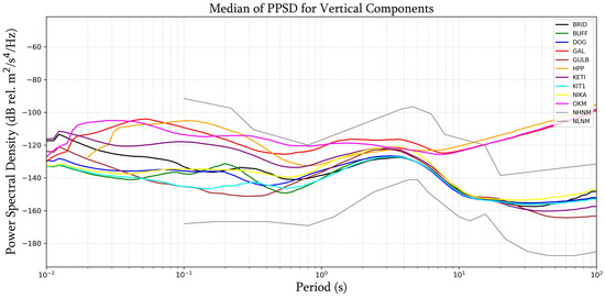
Figure 2.
Median power spectral density (PPSD) for vertical component across all stations compared with Peterson noise models.
The PPSD analysis confirms and complements the Vrms-based observations: stations KIT1, BUFF, NIKA, DOG, and GULB exhibit spectral noise levels that closely approach the New Low Noise Model (NLNM) across the entire seismic frequency band. In contrast, the surface stations GAL, KETI, OKM, and HPP show elevated noise levels over a broad portion of the spectrum (until 10 s), reflecting more exposed or less shielded installation environments. Nevertheless, all stations remain below the New High Noise Model (NHNM), confirming that even the noisiest sites in the Enguri network operate within globally accepted noise limits.
Together, the Vrms and PPSD analyses provide a coherent and detailed characterization of ambient noise variability across the Enguri seismic network, underpinning data quality assessment, magnitude completeness evaluation, and microseismic detectability throughout the monitored area.
Although ambient noise studies commonly rely on power spectral density (PSD) values in acceleration units, root-mean-square velocity (Vrms) estimates in m/s provide an intuitive and practical complement for evaluating station performance, particularly within local networks. Similar methods have been employed to assess broadband station quality and sensor performance [27,28,29]. While formal Vrms-based noise thresholds are not yet standardized in the literature, the values reported in this study fall within the expected range for well-installed broadband and borehole sensors. This analytical framework is consistent with widely adopted methodologies for ambient noise benchmarking and instrumental self-noise characterization [30].
3.3. Local Magnitude Estimation and Uncertainty
The local magnitude (ML) for each event was calculated using the SEISAN software, which applies a standard Richter-type formulation [31] and was later adapted for regional seismic networks [32]. The implementation used in this study follows the methods described in [33], as part of the SEISAN processing framework. Although this method is not specifically calibrated for the Enguri region, it was applied consistently across all events. This uniform application ensures that any systematic bias in absolute magnitudes remains constant, thereby preserving the internal relative scaling essential for statistical analyses such as Gutenberg–Richter b-value estimation, Allan factor calculations, and time clustering metrics.
For each event, ML was independently computed at each station that recorded it. The final event magnitude was defined as the average of the station-specific ML values. The associated magnitude uncertainty was quantified as the standard deviation of these station estimates, reflecting intra-event variability arising from local noise conditions and site amplification effects. Across the analyzed events, this standard deviation typically ranged from 0.1 to 0.3, with a network-wide average uncertainty of approximately 0.23 magnitude units.
To ensure robustness in magnitude determination, only events recorded by at least four stations were included. The number of contributing stations varied between four and eight, depending on event magnitude, location, and signal-to-noise ratio.
Ground conditions—such as surface versus borehole installations and soil versus rock coupling—can significantly affect recorded amplitudes. No site-specific corrections were applied prior to ML estimation. Instead, to mitigate biases from individual stations with potentially amplified ground motions, event magnitudes were computed as averages across all contributing stations. Borehole sites (e.g., KIT1, BUFF, DOG, and NIKA) typically exhibited lower noise levels and more stable amplitude readings, thereby contributing to more reliable magnitude estimates. Future improvements will incorporate station-specific corrections based on empirical site response functions or values, pending further site characterization.
Two illustrative examples (Figure 3 and Figure 4) highlight how site conditions affect amplitude and magnitude variability. We present recordings of two local microearthquakes, observed at six stations, which occurred on 13 February 2023 (ML = 0.8, Lat: 42.762, Lon: 41.987) and 13 March 2023 (ML = 1.0, Lat: 42.764, Lon: 42.031). The recordings come from the following stations: KIT1, a deep borehole station (250 m, Trillium Compact 20s); GULB, a surface broadband station on a concrete pedestal (MBB-2); and KETI, a surface broadband station on soft soil (MBB-2). Waveforms were bandpass-filtered between 5 and 10 Hz.
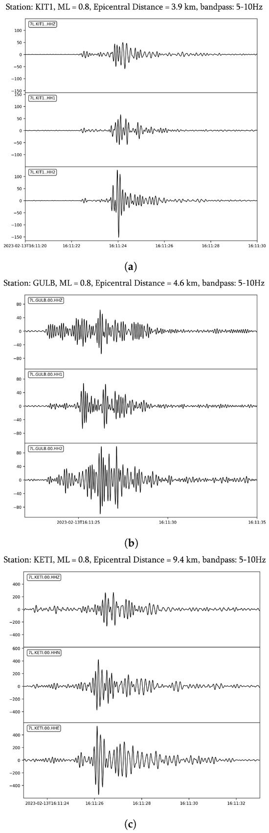
Figure 3.
Event recordings on three seismic stations: (a) KITI, (b) GULB, (c) KETI. Records of the 13 February 2023 event (ML = 0.8; Lat: 42.762, Lon: 41.987, Depth = 8.7 km).
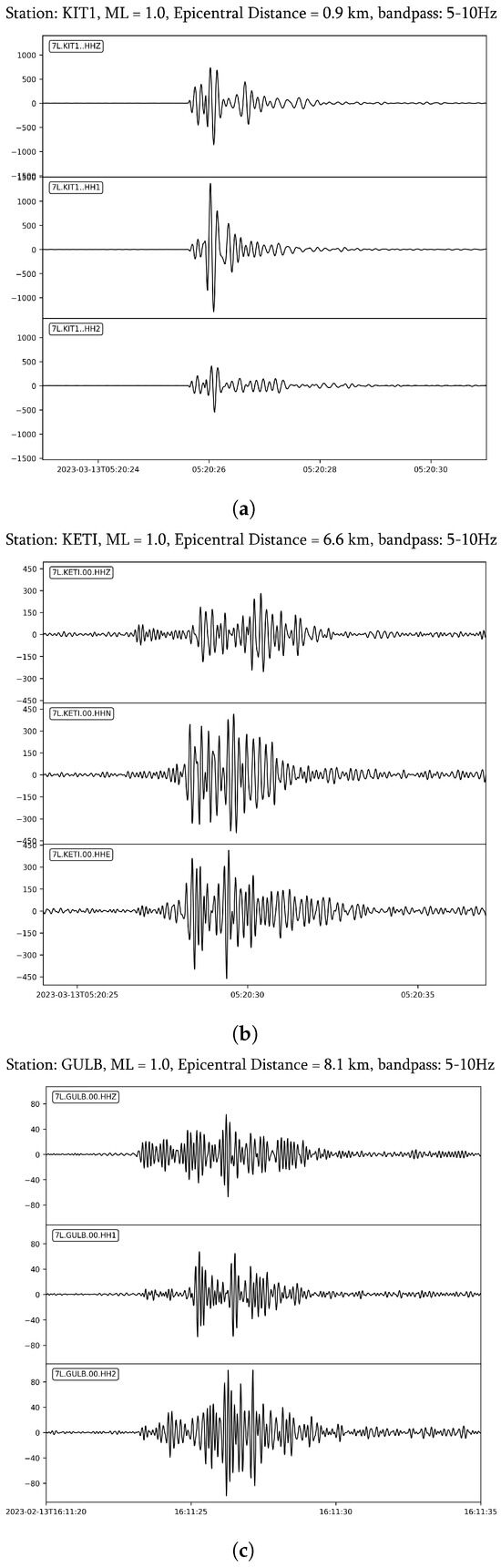
Figure 4.
Event recordings on three seismic stations: (a) KITI, (b) KETI, (c) GULB. Records of the 13 March 2023 event (ML = 1.0; Lat: 42.764, Lon: 42.031, Depth = 3.1 km).
For the first event, KIT1 exhibited the lowest ambient noise and the most stable amplitudes, making it ideal for reliable ML estimation. In contrast, KETI recorded significantly higher amplitudes, likely due to site amplification and resonance effects associated with its soft-soil installation, despite being at a slightly greater epicentral distance. GULB showed intermediate waveform characteristics. The resulting magnitude uncertainty for this event, calculated as the standard deviation across stations, was 0.28.
For the second event, signal amplitudes at KETI were not markedly amplified, resulting in reduced inter-station variability. The associated magnitude uncertainty in this case was 0.23.
These examples illustrate the variability of amplitude-based magnitude estimates across stations with differing site conditions. By applying consistent preprocessing, multi-station averaging, and maintaining a well-distributed network geometry, this study ensures that such variability does not significantly affect the statistical integrity of the catalog. Given that the primary objectives focus on temporal and structural seismicity analyses rather than absolute source scaling, the adopted approach provides sufficient accuracy and robustness. Regional calibration of the ML scale remains a target for future work.
4. Methods
4.1. The Frequency–Magnitude Distribution
The Gutenberg–Richter (GR) law [34] describes the relationship between the number of earthquakes, N, with a magnitude greater than or equal to a threshold magnitude and the threshold. It is given by the equation
The coefficient b plays a crucial role as it reflects the proportion between smaller and larger events, and it also informs about the stress state within the Earth’s crust. Estimating precisely the b-value is essential for an accurate assessment of seismic hazard [35,36].
The b-value can be estimated by using the least square linear regression (LSR) method on the logarithm of the cumulative number of earthquakes with [37], where is the completeness magnitude of the earthquake catalog corresponding to the smallest magnitude that can be detected by the seismic network [38], as follows:
Its error is given by the following formula:
where represents the linear regression estimate of .
plays an important role in the estimation of b. can be calculated by using several methods. In particular, by the method of maximum curvature (MAXC) [39], is the magnitude corresponding to the largest frequency of seismic events in the non-cumulative binned frequency–magnitude distribution. In the goodness-of-fit test (GFT) method [39], is estimated by comparing the frequency–magnitude distribution of the observed seismicity with those of synthetic earthquake sequences. The synthetic distributions are generated based on the a and b values estimated from the observed dataset for magnitudes , evaluated as the cutoff magnitude increases. Let R represent the absolute difference in earthquake counts per magnitude bin between the observed and synthetic distributions. The magnitude of completeness, , is defined as the smallest for which the observed data for align with a straight line on a log-linear plot, within a specified confidence threshold given by .
4.2. The Allan Factor
A set of earthquakes can be modeled by a discrete-time point process marked by the magnitude
where is the time of occurrence of the event i with magnitude .
By partitioning the time axis into non-overlapping intervals of duration , referred to as the timescale, we construct the sequence , which is the series the number of earthquakes occurring within the k-th time window [40].
The AF is defined by the following formula:
The AF was employed in the investigation the time dynamics of several phenomena [41,42,43,44]. In a Poissonian seismic sequence, where events are independent and uncorrelated, the AF remains relatively flat across all considered timescales, oscillating around a value of 1, except at very large timescales where finite-size effects become significant [45,46]. In contrast, a clustered earthquake sequence exhibits an AF that varies with the timescale , typically increasing following a power-law trend, as expected in a fractal (self-similar) process.
In this case, the exponent of the power-law , known as fractal exponent, measures the strength of time clusterization; is called fractal onset time and marks the smaller limit of significant scaling behavior in the AF [40]. Thus, if , the earthquake sequence can be considered Poissonian, while if , it is clusterized.
4.3. The Global and Local Coefficient of Variation
If an earthquake series is represented by the sequence of the interoccurrence intervals, the following quantities can be defined: the global coefficient of variation [47]
and the local coefficient of variation [48]
where is the series of the interoccurrence times and and are their standard deviation and mean.
These two metrics are both employed to assess the degree of time clustering within an earthquake sequence. In the case of a Poissonian process, where events are randomly distributed, both and take on values close to 1. For regular or periodic sequences, these values drop below 1, indicating reduced variability, whereas for clustered sequences, they exceed 1. The coefficient of variation, , reflects the overall clustering behavior of the sequence and can be influenced by fluctuations in the event rate. On the other hand, the local variation, , captures the variability between successive interevent times and is less sensitive to gradual changes in the average rate. For example, if two periodic sequences are concatenated, the combined sequence may appear strongly clustered on a global scale—resulting in —but remains locally periodic, leading to .
4.4. The Detrended Fluctuation Analysis
Detrended fluctuation analysis (DFA) was introduced as a method to identify long-range correlations in non-stationary signals [49], and it has since been extensively employed [50,51,52,53,54]. Telesca et al. [55] used DFA to analyze earthquake magnitudes and discovered that the scaling exponent of the fluctuation function augmented during the reactivation phases of volcanic activity at El Hierro (Spain) from 2011 to 2014. Varotsos et al. [56] considered DFA results for earthquake magnitudes as a tool for forecasting earthquakes. Additionally, Lennartz et al. [57] studied the long-range correlations in the earthquake magnitudes in Northern and Southern California using DFA. Varotsos et al. [58] demonstrated that the DFA scaling exponent in California’s seismicity could indicate disruptions in long-range correlations preceding major seismic events.
The scaling behavior of seismic interevent time series has been examined in various studies using DFA [59]. Investigating long-range correlations in both earthquake magnitudes and interevent times is therefore a key approach for understanding the underlying dynamics of seismic activity.
The DFA method is described below:
- The series , where , and N is the size of the series, is integrated and the integrated series is divided into boxes of equal size n.
- For each n-size box, a line fits by the least square method and is subtracted from .
- The fluctuation, , is calculated as
- Steps (i)–(iii) are repeated for all the available box sizes n. A power-law relationship between and n indicates the presence of long-range correlation in the series, as follows:
- The numerical value of the scaling exponent provides insight into the temporal correlation structure of the seismic series, as follows:
- If , the series is uncorrelated.
- If , the series exhibits persistent correlations, meaning that an increase (or decrease) in one period is likely to be followed by a similar trend in the next.
- If , the series displays antipersistent correlations, where an increase is typically followed by a decrease, and vice versa.
4.5. The Natural Visibility Graph
The Natural Visibility Graph (NVG) transforms a time series into a graph or network. Two arbitrary data points, and , are considered connected nodes in the corresponding graph if any other data point located between them satisfies the condition given by [18]
The NVG method has been utilized across various research areas, including economics [60,61,62], weather forecasting [63,64], medicine [65,66,67], earthquakes [68], biology [69], among others. One of the key parameters in the NVG method is the degree, which indicates the number of connections originating from a node. Typically, higher values in the series function as hubs within the graph, as they tend to “attract” more connections compared with nodes associated with lower values.
An earthquake sequence can be examined using the NVG method by treating the magnitudes as nodes of a graph and establishing links between magnitudes that satisfy the “visibility” criterion (Equation (11)). In this way, a seismic sequence can be transformed into a graph using the NVG method.
The adjacency matrix describes the connections between nodes as follows:
Considering two time series with adjacency matrices and , the (AEO) [70,71] is given by
where is the Kronecker delta. can vary between 1 (when both the adiacency matrices are identical) and (when each edge exists just for one VG); we can interpret these two conditions like the maximum of correlation and the absence of correlation among the variables, respectively.
The AEO defined in Equation (13) can be used to estimate the time-lag between two series. Given two time series and , keeping the first fixed, we construct the time-shifted copies of the second one, . For and each of the time-shifted copies of , we calculate the adjacency matrix, obtained by applying Equation (11). Indicating as the adiacency matrix of and as , , , etc., the adjacency matrices of the delayed copies of , from the maximum of sequence , the time-lag between the series and can be derived. As an example, consider two sinusoids with delay , and , where and represent white noise with and variances and , respectively (Figure 5a). Plotting between the two sinusoids, the maximum is at , which is exactly the delay of the second sinusoid with respect to the first one (Figure 5b).
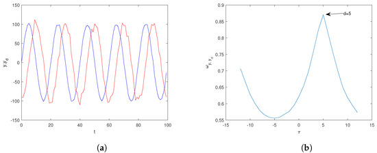
Figure 5.
(a) Comparison between two sinusoids with delay , and , where and represent white noise with and variances and , respectively. (b) Variation of with the time lag ; the maximum of indicates the time lag of between the two sinusoids.
4.6. The Correlogram-Based Periodogram
For short time series, an effective algorithm for computing the power spectrum is the correlogram-based periodogram.
Consider the simple model of periodic series, as follows:
with > 0, , distributed as a uniform variable in , and being a series of uncorrelated random variables with mean 0 and standard deviation , independent of .
The classical periodogram is given by
where N is the length of the series, and it is calculated for
where and indicates the integer part of x. If the series is modulated by a strong cycle with frequency , the periodogram will display a peak at . In contrast, for an uncorrelated series (), the periodogram remains nearly flat, with no distinct peak [72]. Ahdesmäki et al. [73] introduced the correlogram-based periodogram, which is more effective than the classical periodogram in identifying the main cycle of a series.
The classical periodogram is equivalent to the correlogram
where
is the estimator of the autocorrelation function. Using the sample autocorrelation function
where indicates the mean, Ahdesmäki et al. [73] proposed the following correlogram-based periodogram to estimate the power spectrum of a series:
where denotes the real part of x, N is the length of the series, and is the biased Spearman’s rank correlation coefficient. In contrast with the standard periodogram, the correlogram-based periodogram can take on negative values, so the absolute value is typically considered.
To test a frequency , the g-statistics can be used, as follows:
If g is large, the tested frequency is considered highly significant. To assess the significance of the tested frequency, a simulation-based method can be applied [73]: a series of random sequences, modeled as in Equation (14), are generated. For each simulated series, the g-value is computed using Equation (21). The distribution of the g-statistics is then estimated from all the calculated g-values, and the p-value is determined. A low p-value indicates the presence of a strong periodicity.
5. Results
A total of 474 seismic events were recorded in the vicinity of the Enguri Dam, with magnitudes ranging from −1.3 to 2.8. Figure 6 shows the time distribution of the analyzed seismicity. The frequency–magnitude distribution of the investigated seismicity is shown in Figure 7. The completeness magnitude was found to be 0.4 for both the MAXC and GFT (with = 90%) methods. The b-value was calculated as using Equation (2). Although the value of b suggests that the Enguri Dam area may be in a relatively stable state, there could exist possible localized stress accumulation possibly near active faults or stress concentration zones influenced by the dam.
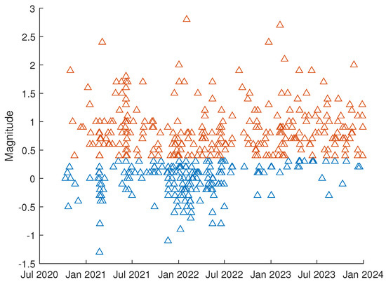
Figure 6.
Time distribution of the earthquakes in the investigated area. The red triangles represent the earthquakes above the completeness magnitude.
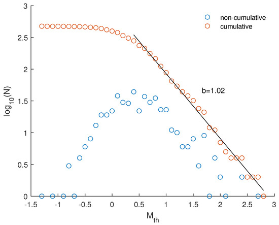
Figure 7.
Cumulative (red) and non-cumulative (blue) frequency–magnitude distribution of earthquakes occurring at depths of up to 30 km and within a 33 km radius from the center of the dam. The slope of the regression line (black) is the estimate of the b-value.
We selected only those earthquakes with magnitude ; thus, the number of analyzed earthquakes reduced from 474 to 279 (represented by the red triangles in Figure 6) and occurred at depths of up to 30 km and within a maximum distance of 33 km from the center of the dam. Various statistical analyses were applied to this dataset with the objective of achieving the most comprehensive characterization possible of the temporal dynamics of the seismic activity around the Enguri Dam.
Figure 8 presents the sequence of interoccurrence times (in days). The global and local coefficients of variation are and , respectively. The 95% confidence intervals for these estimates, [0.888, 1.138] and [0.875, 1.116], were determined based on 100 simulated Poissonian seismic sequences, which match the original dataset in size and mean interoccurrence time. These intervals were derived as the 2.5% and 97.5% percentiles of the and distributions calculated from the Poissonian sequences. Since the and values for the Enguri seismicity exceed their respective 95% confidence intervals, the analyzed earthquakes exhibit a time-clustered process on both global and local scales, meaning that earthquakes tend to occur in clusters rather than randomly over time. The local coefficient of variation is even larger than the global one, which could suggest stress accumulation and release cycles in certain fault segments, as well as hydro-seismic effects due to water level changes.
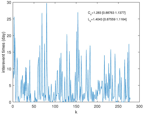
Figure 8.
Sequence of the interoccurrence times.
Figure 9 displays the Allan factor (AF) for the analyzed seismic activity alongside the 95% confidence bands corresponding to two types of surrogate sequences: 100 Poissonian sequences sharing the same rate as the original dataset (in green) and 100 randomized sequences produced by shuffling the original interoccurrence times, preserving the same probability density function of interoccurrence times, (in red). The AF slightly increases with the timescale , indicating that the seismicity exhibits a certain degree of time clusterization. However, from the numerical value of the scaling exponent , which quantifies the strength of the clusterization, estimated over the range of the large timescales, such clustering appears rather weak. Except the range of very large timescales, where the AF is characterized by a certain fluctuating behavior, it significantly exceeds the Poissonian 95% confidence band, indicating non-Poissonian behavior across the considered timescales. However, the AF remains within the 95% confidence interval derived from the 100 random shuffles, suggesting that the clustering behavior could be very likely due to the behavior of the . The AF results might suggest that microearthquakes near the high dam could exhibit a noticeable time clustering that is weak, meaning that there is no strong external trigger. However, the results leave open the possibility that subtle processes like pore pressure changes or small stress redistributions due to reservoir loading/unloading may play a role in shaping the seismicity pattern.
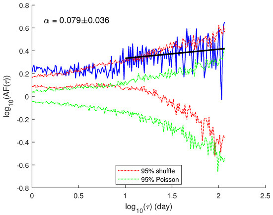
Figure 9.
The Allan factor of the earthquake sequence is shown in blue. The red dotted lines indicate the 95% confidence interval derived from random shuffles of the original interevent times, while the green dotted lines represent the 95% confidence interval based on Poissonian surrogate sequences. The black solid line shows the linear regression of the Allan factor over the larger timescales, with its slope corresponding to the fractal exponent.
Figure 10 illustrates the fluctuation function for both the interoccurrence times (Figure 10a) and the magnitudes (Figure 10b). The interoccurrence times exhibit a mildly persistent behavior, suggesting that an increase or decrease in the interoccurrence time during one period is likely to be followed by a similar trend in the subsequent period. This suggests that past seismic activity slightly influences future events, potentially due to periodic stress accumulation and release near the dam. Fluctuations in reservoir water levels can alter the stress state of surrounding rock, gradually increasing pressure until microearthquakes are triggered. This process appears not entirely random but exhibits some memory of prior seismic events—implying that once stress is accumulated, it may require time to be released again, resulting in clustered seismic activity. While the timing of earthquakes shows such memory effects, the magnitudes do not exhibit any clear temporal pattern. This supports the notion that earthquake sizes follow statistical distributions rather than being governed by a predictable process.
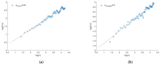
Figure 10.
Detrended fluctuation analysis of the (a) interoccurrence times and (b) magnitudes. the red dotted lines show the linear regression of the fluctuation function over the scale n.
We analyzed the seismic dataset by means of the NVG method. Figure 11a shows the links among the magnitudes drawn on the base of the “visibility” criterion of Equation (11).
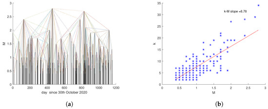
Figure 11.
(a) Sequence of analyzed earthquakes. The links among the magnitudes are defined by the Natural Visibility Graph. (b) Relationship between the degree k and the magnitude M.
Following Telesca et al. [74], who identified an intriguing relationship between the degree k in a seismic sequence and earthquake magnitude M, the slope of the linear fit describing this relationship is referred to as the k–M slope. Several studies using observational [75], experimental [20], and physics-based synthetic [76] seismic catalogs have reported a positive correlation between the k–M slope and the Gutenberg–Richter b-value. More recently, Li et al. [77] demonstrated that this correlation is both universal and stable.
Figure 11b illustrates the relationship between the degree k and magnitude M in our earthquake dataset, along with the corresponding linear regression line. The slope of this fit, known as the k–M slope, is positive (), indicating a direct correlation between degree and magnitude. In other words, larger-magnitude earthquakes tend to have higher degrees—they function as “hubs” in the seismic network, drawing more connections than smaller events, and are thus “visible” to more earthquakes.
Moreover, Figure 12 shows that the Enguri seismic dataset aligns well with the general trend observed in other seismic datasets, further supporting the robustness of the k–M slope–b-value relationship.
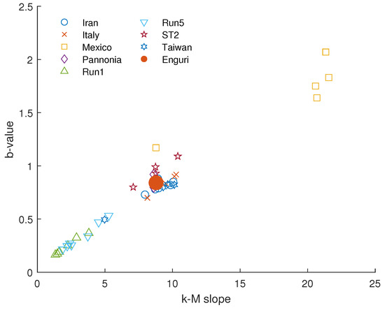
Figure 12.
Relationship between the k-M slope and the b-value for the Enguri dataset compared with that of the seismic datasets analyzed in previous studies (Iran [19], Italy and Taiwan [20], Mexico [74], Pannonia [78], R1 and R2 [79], and ST2 [80]).
Figure 13 illustrates the monthly changes in the number of earthquakes (with ) alongside the monthly average water level of the Enguri reservoir. The monthly variation in earthquake frequency remains below 20 events per month. Meanwhile, the average water level is characterized by a distinct annual cycle. This cyclical behavior is further supported by correlogram-based periodogram analysis. Figure 14 displays the correlogram-based periodogram for the monthly mean water level (in yellow) and the monthly earthquake counts (in blue); the 99% significant periods are indicated by circles. The water level exhibits a clear and significant quasi-annual periodicity, which is also mirrored in the monthly earthquake counts, though with less intensity. However, given the availability of the water level time series starting from 1978, we applied the correlogram-based method to the entire dataset in order to accurately determine the periodicity of the monthly water level. The resulting spectrum, shown in Figure 15, indicates that the dominant periodicity is 12 months. A secondary peak at 6 months is present and represents a harmonic of the annual cycle.
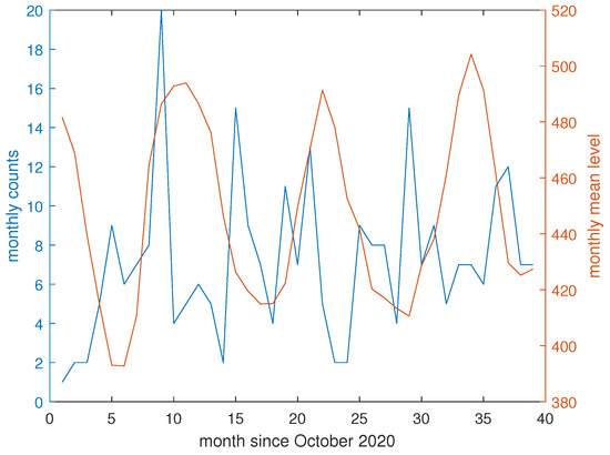
Figure 13.
Time variation of the monthly earthquake counts (blue) and mean water level (red).
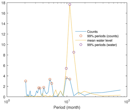
Figure 14.
Correlogram-based periodogram of the monthly earthquake counts (blue) and the monthly mean water level (yellow). The circles indicates the 99% significant periods in both periodograms.
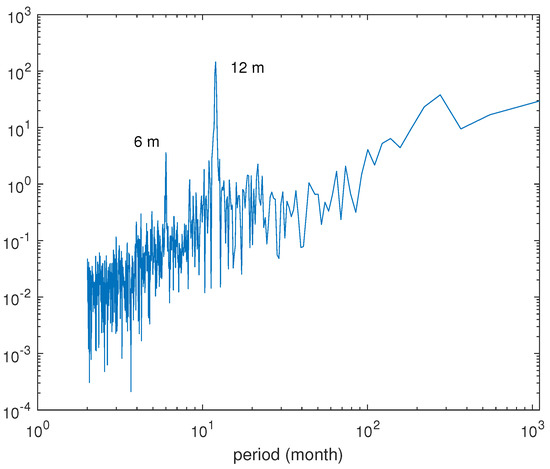
Figure 15.
Correlogram-based periodogram of the monthly mean water level from 1978 to 2023. The dominant periodicity occurs at 12 months, corresponding to the main cycle, while the 6-month peak represents its first harmonic.
We applied the NVG to both monthly time series and computed the AEO while varying the time lag from −12 to 12 months.
To evaluate the significance of the obtained values, we constructed a null distribution representing the case of no correlation between the two graphs. This was implemented using a permutation-based approach, structured as follows:
- The adjacency matrices of both graphs were randomly permuted, while preserving the null elements on the diagonal and maintaining symmetry. These constraints ensure that node connections are shuffled randomly, but the overall graph structure remains consistent with the visibility graph rules.
- For each permutation and time lag , the value was computed.
- This process was repeated 100 times, resulting in a null distribution of values for each time lag .
- The 95th percentile of each distribution was calculated to determine the threshold for statistical significance.
- These percentiles were then used to construct a 95% confidence envelope for . If the observed value exceeds this envelope at a given , it is considered statistically significant.
The results shown in Figure 16 indicate a significant correlation between the two time series, with consistently remaining above the 95% confidence curve for all values of . Notably, the highest value of is observed at months, indicating that the monthly mean water level leads the monthly earthquake counts by approximately 7 months (±0.5 months, considering the monthly resolution of the time series). This result further supports the possibility that seismic activity around the Enguri reservoir may be influenced by the loading and unloading cycles associated with reservoir operations, which, although not dominant, could play a contributing role in triggering observed seismic events. Furthermore, the found delay would strengthen the hypothesis that the triggering mechanism by which the dam influences fault activation—already critically stressed by the tectonic stress field—is not the immediate undrained elastic response to loading, but rather a delayed seismic response driven by the diffusion of pore fluid pressures.
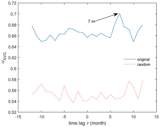
Figure 16.
Average edge overlap between the monthly time series of earthquake counts and mean water level. The red dotted line represents the 95% confidence curve.
The effect of the annual loading/unloading of the dam can be approximated by a periodic pore-pressure variation at the base of the dam. This can be expressed as
where T is the period of the loading/unloading cycle. Following Saar and Manga [81], the hydraulic diffusivity D can be expressed as
where h is the mean depth of the seismic events, is given by Equation (22), and is the time delay between water level and seismicity (which in our case are the monthly mean water level and earthquake counts, respectively).
In our case, months (as shown in Figure 15), (as shown in Figure 16), and . Substituting these values into Equation (23) gives
This estimated value of D falls within the typical range of seismic hydraulic diffusivity (0.1–100 m2/s) reported by Talwani and Acree [82] in their study of seismicity near the Monticello Reservoir (Italy).
6. Conclusions
In this study, we conducted several statistical analyses on microearthquake seismicity in the Enguri area (Georgia) that occurred between 2020 and 2023. These events were recorded by a newly installed seismic network developed as part of the DAMAST project. The enhanced sensitivity of this network enabled the detection of even very small seismic events, allowing a more detailed picture of the temporal dynamics of seismicity in the area. Our main findings can be summarized as follows: (1) the seismicity around the Enguri Dam is likely influenced by a combination of natural tectonic processes and subtle reservoir-induced stress changes; (2) although the dam does not appear to be causing strong seismic forcing, it could have a role in triggering the seismicity that appears to be delayed by about 7 months from the water level; (3) localized stress variations and time clustering suggest that water level changes may modulate seismic activity over time; and (4) the mild persistence of interoccurrence times aligns with the idea of stress buildup and delayed earthquake triggering due to reservoir loading effect.
Author Contributions
Conceptualization, L.T.; methodology, L.T.; software, L.T.; formal analysis, L.T.; investigation, L.T., T.C. and N.T. (Nino Tsereteli); data curation, N.T. (Nino Tsereteli) and N.T. (Nazi Tugushi); writing—original draft preparation, L.T. and N.T. (Nino Tsereteli); writing—review and editing, L.T., T.C. and N.T. (Nino Tsereteli); visualization, L.T., N.T. (Nino Tsereteli) and N.T. (Nazi Tugushi). All authors have read and agreed to the published version of the manuscript.
Funding
This research was funded by the National Research Council (93C23000100005) and by the Shota Rustaveli National Science Foundation of Georgia (FR-21-20840).
Data Availability Statement
Seismicity and water level data are provided in the publicly accessible RADAR4KIT data repository under DOI: 10.35097/ms4mgwspyvbggw6k and DOI: 10.35097/qmczxs93wh0vz407, respectively.
Acknowledgments
The authors would like to thank the Federal Ministry of Education and Research of Germany (BMBF, now BMFTR) for funding the DAMAST and DAMAST-Transfer projects as part of ‘CLIENT II—International Partnership for Sustainable Innovations’, a funding programme within the framework of ‘Research for Sustainable Development (FONA3)’, BMBF project 03G0882A—DAMAST and DAMAST transfer. This enabled to establish the new station network.
Conflicts of Interest
The authors declare no conflicts of interest.
References
- Reilinger, R.; McClusky, S.; Vernant, P.; Lawrence, S.; Ergintav, S.; Cakmak, R.; Ozener, H.; Kadirov, F.; Guliev, I.; Stepanyan, R.; et al. GPS constraints on continental deformation in the Africa-Arabia-Eurasia continental collision zone and implications for the dynamics of plate interactions. J. Geophys. Res. Solid Earth 2006, 111, 1–26. [Google Scholar] [CrossRef]
- Allen, M.; Jackson, J.; Walker, R. Late Cenozoic reorganization of the Arabia-Eurasia collision and the comparison of short-term and long-term deformation rates. Tectonics 2004, 23, 1–16. [Google Scholar] [CrossRef]
- Mosar, J.; Kangarli, T.; Bochud, M.; Glasmacher, U.A.; Rast, A.; Brunet, M.F.; Sosson, M. Cenozoic-recent tectonics and uplift in the greater Caucasus: A perspective from Azerbaijan. Geol. Soc. Spec. Publ. 2010, 340, 261–280. [Google Scholar] [CrossRef]
- Zor, E.; Sandvol, E.; Gürbüz, C.; Türkelli, N.; Seber, D.; Barazangi, M. The crustal structure of the East Anatolian Plateau (Turkey) from receiver functions. Geophys. Res. Lett. 2006, 33, L08301. [Google Scholar] [CrossRef]
- Copley, A.; Jackson, J. Active tectonics of the Turkish–Iranian Plateau. Tectonics 2006, 25, TC6006. [Google Scholar] [CrossRef]
- Mcclusky, S.; Balassanian, S.; Barka, A.; Demir, C.; Ergintav, S.; Georgiev, I.; Gurkan, O.; Hamburger, M.; Hurst, K.; Kahle, H.; et al. Global positioning system constraints on plate kinematics and dynamics in the eastern Mediterranean and Caucasus. J. Geophys. Res. Solid Earth 2000, 105, 5695–5719. [Google Scholar] [CrossRef]
- Aktuğ, B.; Meherremov, E.; Kurt, M.; Özdemir, S.; Esedov, N.; Lenk, O. GPS constraints on the deformation of Azerbaijan and surrounding regions. J. Geodyn. 2013, 67, 40–45. [Google Scholar] [CrossRef]
- Kadirov, F.; Gadirov, A.; Abdullayev, N. Gravity modelling of the regional profile across South Caspian basin and tectonic implications. In The Modern Problems of Geology and Geophysics of Eastern Caucasus and the South Caspian Depression; Nafta-Press: Baku, Azerbaijan, 2012; Volume 231, p. 251. [Google Scholar]
- Müller, M.; Asch, G.; Ratschbacher, L.; Stöckhert, B.; Zor, E.; Akal, C.; Sipahioglu, S.; Lueth, S.; Kind, R. Present-day deformation across the Lesser and Greater Caucasus from geodetic and seismological data. Earth Planet. Sci. Lett. 2022, 579, 117369. [Google Scholar]
- Sokhadze, G.; Floyd, M.; Godoladze, T.; King, R.; Cowgill, E.; Javakhishvili, Z.; Hahubia, G.; Reilinger, R. Active convergence between the lesser and greater Caucasus in Georgia: Constraints on the tectonic evolution of the lesser-greater Caucasus continental collision. Earth Planet. Sci. Lett. 2018, 481, 154–161. [Google Scholar] [CrossRef]
- Caputo, M.; Gamkrelidze, I.; Malvezzi, V.; Sgrigna, V.; Shengelaia, G.; Zilpimiani, D. Geostructural basis and geophysical investigations for the seismic hazard assessment and prediction in the Caucasus. Il Nuovo Cimento C 2000, 23, 191–216. [Google Scholar]
- Philip, H.; Cisternas, A.; Gvishiani, A.; Gorshkov, A. The Caucasus: An actual example of the initial stages of continental collision. Tectonophysics 1989, 161, 1–21. [Google Scholar] [CrossRef]
- Tan, O.; Taymaz, T. Active tectonics of the Caucasus: Earthquake source mechanisms and rupture histories obtained from inversion of teleseismic body waveforms. Spec. Pap. Geol. Soc. Am. 2006, 409, 531. [Google Scholar]
- Telesca, L.; Tsereteli, N.; Chelidze, T.; Lapenna, V. Spectral investigation of the relationship between seismicity and water level in the Enguri high dam area (Georgia). Geosciences 2024, 14, 22. [Google Scholar] [CrossRef]
- Karamzadeh, N.; Tsereteli, N.; Gaucher, E.; Tugushi, N.; Shubladze, T.; Varazanashvili, O.; Rietbrock, A. Seismological study around the Enguri dam reservoir (Georgia) based on old catalogs and ongoing monitoring. J. Seismol. 2023, 27, 953–977. [Google Scholar] [CrossRef]
- Braun, T.; Cesca, S.; Kuhn, D.; Martirosian-Janssen, A.; Dahm, T. Anthropogenic seismicity in Italy and its relation to tectonics: State of the art and perspectives. Anthropocene 2018, 21, 80–94. [Google Scholar] [CrossRef]
- Basili, R.; Danciu, L.; Beauval, C.; Sesetyan, K.; Vilanova, S.P.; Adamia, S.; Arroucau, P.; Atanackov, J.; Baize, S.; Canora, C.; et al. The European Fault-Source Model 2020 (EFSM20): Geologic input data for the European Seismic Hazard Model 2020. Nat. Hazards Earth Syst. Sci. 2024, 24, 3945–3976. [Google Scholar] [CrossRef]
- Lacasa, L.; Luque, B.; Ballesteros, F.; Luque, J.; Nuno, J.C. From time series to complex networks: The visibility graph. Proc. Natl. Acad. Sci. USA 2008, 105, 4972–4975. [Google Scholar] [CrossRef]
- Khoshnevis, N.; Taborda, R.; Azizzadeh-Roodpish, S.; Telesca, L. Analysis of the 2005–2016 earthquake sequence in Northern Iran using the visibility graph method. Pure Appl. Geophys. 2017, 174, 4003–4019. [Google Scholar] [CrossRef]
- Telesca, L.; Chen, C.C.; Lovallo, M. Investigating the relationship between seismological and topological properties of seismicity in Italy and Taiwan. Pure Appl. Geophys. 2020, 177, 4119–4126. [Google Scholar] [CrossRef]
- Kobalia, O.; Gogokhia, K.; Kalabegishvili, M. Water Level of the Jvari Reservoir of Enguri High Arch Dam for the Years 1978–2025; Engurhesi Ltd.: Tbilisi, Georgia, 2025. [Google Scholar]
- Frietsch, M.; Tugushi, N.; Karamzadeh, N.; Tsereteli, N.; Gaucher, E.; Rietbrock, A. Seismisches Monitoring im Betrieb der Enguri-Stauanlage. Z. Für Wasserwirtsch. 2025; in preparation. [Google Scholar]
- Murusidze, G. Seismicity and the possible position of strong earthquakes sources in the area of the Inguri HPP. In Seismic Impacts on Hydrotechnical and Power Structures; Savarensky, E., Ed.; Pub, House Nauka: Moscow, Russia, 1980; pp. 73–80. [Google Scholar]
- McNamara, D.E.; Buland, R.P. Ambient noise levels in the continental United States. Bull. Seismol. Soc. Am. 2004, 94, 1517–1527. [Google Scholar] [CrossRef]
- Krischer, L.; Megies, T.; Barsch, R.; Beyreuther, M.; Lecocq, T.; Caudron, C.; Wassermann, J. ObsPy: A bridge for seismology into the scientific Python ecosystem. Comput. Sci. Discov. 2015, 8, 014003. [Google Scholar] [CrossRef]
- Peterson, J. Observations and Modeling of Seismic Background Noise; U.S. Geological Survey Open-File Report 93-322; U.S. Geological Survey: Reston, VA, USA, 1993. [CrossRef]
- Ringler, A.T.; Hutt, C.R. Self-Noise Models of Seismic Instruments. Seismol. Res. Lett. 2010, 81, 972–983. [Google Scholar] [CrossRef]
- Anthony, R.E.; Ringler, A.T.; Wilson, D.C.; McNamara, D.E. Ambient Noise Levels in the Continental United States. Seismol. Res. Lett. 2020, 91, 2199–2210. [Google Scholar]
- Casey, A.T.; Ringler, A.T.; Anthony, R.E. Ambient Seismic Noise as a Measure of Station Performance. Seismol. Res. Lett. 2018, 89, 1453–1460. [Google Scholar] [CrossRef]
- Sleeman, R.; van Wettum, A.; Trampert, J. Three-channel correlation analysis: A new technique to measure instrumental noise of digitizers and seismic sensors. Bull. Seismol. Soc. Am. 2006, 96, 258–271. [Google Scholar] [CrossRef]
- Richter, C.F. An Instrumental Earthquake Magnitude Scale. Bull. Seismol. Soc. Am. 1935, 25, 1–32. [Google Scholar] [CrossRef]
- Hutton, L.K.; Boore, D.M. The ML Scale in Southern California. Bull. Seismol. Soc. Am. 1987, 77, 2074–2094. [Google Scholar] [CrossRef]
- Havskov, J.; Ottemöller, L. SEISAN: The Earthquake Analysis Software for Windows, Solaris, Linux and MacOSX. Seismol. Res. Lett. 2010, 81, 532–540. [Google Scholar]
- Gutenberg, R.; Richter, C.F. Frequency of earthquakes in California. Bull. Seismol. Soc. Am. 1944, 34, 185–188. [Google Scholar] [CrossRef]
- Scholz, C.H. The frequency-magnitude relation of microfracturing in rock and its relation to earthquakes. Bull. Seismol. Soc. Am. 1968, 58, 399–415. [Google Scholar] [CrossRef]
- Wyss, M. Towards a physical understanding of the earthquake frequency distribution. Geophys. J. R. Astron. Soc. 1973, 31, 341–359. [Google Scholar] [CrossRef]
- Kárník, V.; Klíma, K. Magnitude-frequency distribution in the European-Mediterranean earthquake regions. Tectonophysics 1993, 220, 309–323. [Google Scholar] [CrossRef]
- Utsu, T. Representation and analysis of the earthquake size distribution: A historical review and some new approaches. Pageoph 1999, 155, 509–535. [Google Scholar] [CrossRef]
- Wiemer, S.; Wyss, M. Minimum magnitude of completeness in earthquake catalogs: Examples from Alaska, the Western United States, and Japan. Bull. Seismol. Soc. Am. 2000, 90, 859–869. [Google Scholar] [CrossRef]
- Thurner, S.; Lowen, S.B.; Feurstein, M.C.; Heneghan, C.; Feichtinger, H.G.; Teich, M.C. Analysis, synthesis, and estimation of fractal-rate stochastic point processes. Fractals 1997, 5, 565–596. [Google Scholar] [CrossRef]
- Fadel, P.; Barman, S.; Phillips, S.; Gebber, G. Fractal fluctuations in human respiration. J. Appl. Physiol. 2004, 97, 2056–2064. [Google Scholar] [CrossRef]
- Fadel, P.; Orer, H.; Barman, S.; Vongpatanasin, W.; Victor, R.; Gebber, G. Fractal properties of human muscle sympathetic nerve activity. Am. J. Physiol. Circ. Physiol. 2004, 286, H1076–H1087. [Google Scholar] [CrossRef]
- Yuan, Y.; Zhuang, X.T.; Liu, Z.Y.; Huang, W.G. Time–clustering behavior of sharp fluctuation sequences in Chinese stock markets. Chaos Solitons Fractals 2012, 45, 838–845. [Google Scholar] [CrossRef]
- Anteneodo, C.; Malmgren, R.; Chialvo, D. Poissonian bursts in e–mail correspondence. Eur. Phys. J. B—Condensed Matter Complex Syst. 2010, 75, 389–394. [Google Scholar] [CrossRef]
- Telesca, L.; ElShafey Fat ElBary, R.; Amin Mohamed, A.E.E.; ElGabry, M. Analysis of the cross-correlation between seismicity and water level in the Aswan area (Egypt) from 1982 to 2010. Nat. Hazards Earth Syst. Sci. 2012, 12, 2203–2207. [Google Scholar] [CrossRef]
- Serinaldi, F.; Kilsby, C.G. On the sampling distribution of Allan factor estimator for a homogeneous Poisson process and its use to test inhomogeneities at multiple scales. Phys. A Stat. Mech. Its Appl. 2013, 392, 1080–1089. [Google Scholar] [CrossRef]
- Kagan, Y.Y.; Jackson, D.D. Long-Term Earthquake Clustering. Geophys. J. Int. 1991, 104, 117–134. [Google Scholar] [CrossRef]
- Shinomoto, S.; Miura, K.; Koyama, S. A measure of local variation of inter-spike intervals. Biosystems 2005, 79, 67–72. [Google Scholar] [CrossRef]
- Peng, C.K.; Havlin, S.; Stanley, H.E.; Goldberger, A.L. Quantification of scaling exponents and crossover phenomena in nonstationary heartbeat time series. Chaos 1995, 5, 82–87. [Google Scholar] [CrossRef]
- Heneghan, C.; McDarby, G. Establishing the relation between detrended fluctuation analysis and power spectral density analysis for stochastic processes. Phys. Rev. E 2000, 62, 6103–6110. [Google Scholar] [CrossRef]
- Talkner, P.; Weber, R.O. Power spectrum and detrended fluctuation analysis: Application to daily temperatures. Phys. Rev. E 2000, 62, 150–160. [Google Scholar] [CrossRef]
- Kantelhardt, J.W.; Koscielny-Bunde, E.; Rego, H.H.A.; Havlin, S.; Bunde, A. Detecting Long-range Correlations with Detrended Fluctuation Analysis. Phys. A Stat. Mech. Its Appl. 2001, 295, 441–454. [Google Scholar] [CrossRef]
- Colás, A.; Vigil, L.; Vargas, B.; Cuesta-Frau, D.; Varela, M. Detrended Fluctuation Analysis in the prediction of type 2 diabetes mellitus in patients at risk: Model optimization and comparison with other metrics. PLoS ONE 2019, 14, e0225817. [Google Scholar] [CrossRef]
- Zhao, S.; Jiang, Y.; He, W.; Mei, Y.; Xie, X.; Wan, S. Detrended fluctuation analysis based on best-fit polynomial. Front. Environ. Sci. 2022, 10, 1054689. [Google Scholar] [CrossRef]
- Telesca, L.; Lovallo, M.; Lopez, M.C.; Molist, J.M. Multiparametric statistical investigation of seismicity occurred at El Hierro (Canary Islands) from 2011 to 2014. Tectonophysics 2016, 672–673, 121–128. [Google Scholar] [CrossRef]
- Varotsos, P.A.; Sarlis, N.V.; Skordas, E.S. Study of the temporal correlations in the magnitude time series before major earthquakes in Japan. J. Geophys. Res. Space Phys. 2014, 119, 9192–9206. [Google Scholar] [CrossRef]
- Lennartz, S.; Livina, V.N.; Bunde, A.; Havlin, S. Long-term memory in earthquakes and the distribution of interoccurrence times. Europhys. Lett. 2008, 81, 69001. [Google Scholar] [CrossRef]
- Varotsos, P.; Sarlis, N.; Skordas, E. Scale-specific order parameter fluctuations of seismicity before mainshocks: Natural time and detrended fluctuation analysis. Europhys. Lett. 2012, 99, 001. [Google Scholar] [CrossRef]
- Telesca, L.; Chen, C.C. Fractal and spectral investigation of the shallow seismicity in Taiwan. J. Asian Earth Sci. 2019. [Google Scholar] [CrossRef]
- Zhang, R.; Ashuri, B.; Shyr, Y.; Deng, Y. Forecasting construction cost index based on visibility graph: A network approach. Physica A 2018, 493, 239–252. [Google Scholar] [CrossRef]
- Long, Y. Visibility graph network analysis of gold price time series. Physica A 2013, 392, 3374–3384. [Google Scholar] [CrossRef]
- Wang, N.; Li, D.; Wang, Q. Visibility graph analysis on quarterly macroeconomic series of China based on complex network theory. Physica A 2012, 391, 6543–6555. [Google Scholar] [CrossRef]
- Jiang, W.; Wei, B.; Zhan, J.; Xie, C.; Zhou, D. A visibility graph power averaging aggregation operator: A methodology based on network analysis. Comput. Ind. Eng. 2016, 101, 260–268. [Google Scholar] [CrossRef]
- Chen, S.; Hu, Y.; Mahadevan, S.; Deng, Y. A visibility graph averaging aggregation operator. Physica A 2014, 403, 1–12. [Google Scholar] [CrossRef]
- Yu, M.; Hillebrand, A.; Gouw, A.A.; Stam, C.J. Horizontal visibility graph transfer entropy (HVG-TE): A novel metric to characterize directed connectivity in large-scale brain networks. NeuroImage 2017, 156, 249–264. [Google Scholar] [CrossRef]
- Bhaduri, S.; Ghosh, D. Electroencephalographic data analysis with visibility graph technique for quantitative assessment of brain dysfunction. Clin. EEG Neurosci. 2015, 46, 218–223. [Google Scholar] [CrossRef] [PubMed]
- Ahmadlou, M.; Adeli, H.; Adeli, A. New diagnostic EEG markers of the Alzheimer’s disease using visibility graph. J. Neural Transm. 2010, 117, 1099–1109. [Google Scholar] [CrossRef] [PubMed]
- Aguilar-San Juan, B.; Guzmán-Vargas, L. Earthquake magnitude time series: Scaling behavior of visibility networks. Eur. Phys. J. B 2013, 86, 454. [Google Scholar] [CrossRef]
- Zheng, M.; Domanskyi, S.; Piermarocchi, C.; Mias, G.I. Visibility graph based temporal community detection with applications in biological time series. Sci. Rep. 2021, 11, 5623. [Google Scholar] [CrossRef]
- Lacasa, L.; Nicosia, V.; Latora, V. Network structure of multivariate time series. Sci. Rep. 2015, 5, 15508. [Google Scholar] [CrossRef]
- Carmona-Cabezas, R.; Gómez-Gómez, J.; Ariza-Villaverde, A.B.; Gutiérrez de Ravé, E.; Jiménez-Hornero, F.J. Multiplex Visibility Graphs as a complementary tool for describing the relation between ground level O3 and NO2. Atmos. Pollut. Res. 2020, 11, 205–212. [Google Scholar] [CrossRef]
- Priestley, M.B. Spectral Analysis and Time Series; Academic Press: London, UK; New York, NY, USA, 1981; p. 890. [Google Scholar]
- Ahdesmäki, M.; Lähdesmäki, H.; Pearson, R.; Huttunen, H.; Yli-Harja, O. Robust detection of periodic time series measured from biological systems. BMC Bioinform. 2005, 6, 117. [Google Scholar] [CrossRef]
- Telesca, L.; Lovallo, M.; Ramirez-Rojas, A.; Flores-Marquez, L. Investigating the time dynamics of seismicity by using the visibility graph approach: Application to seismicity of Mexican subduction zone. Physica A 2013, 391, 1553–1562. [Google Scholar] [CrossRef]
- Azizzadeh-Roodpish, S.; Cramer, C.H. Visibility graph analysis of Alaska crustal and Aleutian subduction zone seismicity: An investigation of the correlation between b value and k–M slope. Pure Appl. Geophys. 2018, 175, 4241–4252. [Google Scholar] [CrossRef]
- Perez-Oregon, J.; Lovallo, M.; Telesca, L. Visibility graph analysis of synthetic earthquakes generated by the Olami–Feder–Christensen spring-block model. Chaos 2020, 30, 093111. [Google Scholar] [CrossRef]
- Li, L.; Luo, G.; Liu, M. The K-M Slope: A Potential Supplement for b-Value. Seismol. Res. Lett. 2023, 94, 1892–1899. [Google Scholar] [CrossRef]
- Telesca, L.; Lovallo, M.; Toth, L. Visibility graph analysis of 2002–2011 Pannonian seismicity. Physica A 2014, 416, 219–224. [Google Scholar] [CrossRef]
- Telesca, L.; Lovallo, M.; Ramirez-Rojas, A.; Flores-Marquez, L. Relationship between the frequency magnitude distribution and the visibility graph in the synthetic seismicity generated by a simple stick-slip system with asperities. PLoS ONE 2014, 9, e106233. [Google Scholar] [CrossRef] [PubMed]
- Telesca, L.; Thai, A.T.; Lovallo, M.; Cao, D.T.; Nguyen, L.M. Shannon Entropy Analysis of Reservoir-Triggered Seis-micity at Song Tranh 2 Hydropower Plant, Vietnam. Appl. Sci. 2022, 12, 8873. [Google Scholar] [CrossRef]
- Saar, M.; Manga, M. Seismicity induced by seasonal groundwater recharge at Mt. Hood, Oregon. Earth Planet. Sci. Lett. 2003, 214, 605–618. [Google Scholar] [CrossRef]
- Talwani, P.; Acree, S. Pore pressure diffusion and the mechanism of reservoir-induced seismicity. Pure Appl. Geophys. 1984, 122, 947–965. [Google Scholar] [CrossRef]
Disclaimer/Publisher’s Note: The statements, opinions and data contained in all publications are solely those of the individual author(s) and contributor(s) and not of MDPI and/or the editor(s). MDPI and/or the editor(s) disclaim responsibility for any injury to people or property resulting from any ideas, methods, instructions or products referred to in the content. |
© 2025 by the authors. Licensee MDPI, Basel, Switzerland. This article is an open access article distributed under the terms and conditions of the Creative Commons Attribution (CC BY) license (https://creativecommons.org/licenses/by/4.0/).