


The Role of Disorder in Foreshock Activity


Abstract
1. Introduction
2. The Model
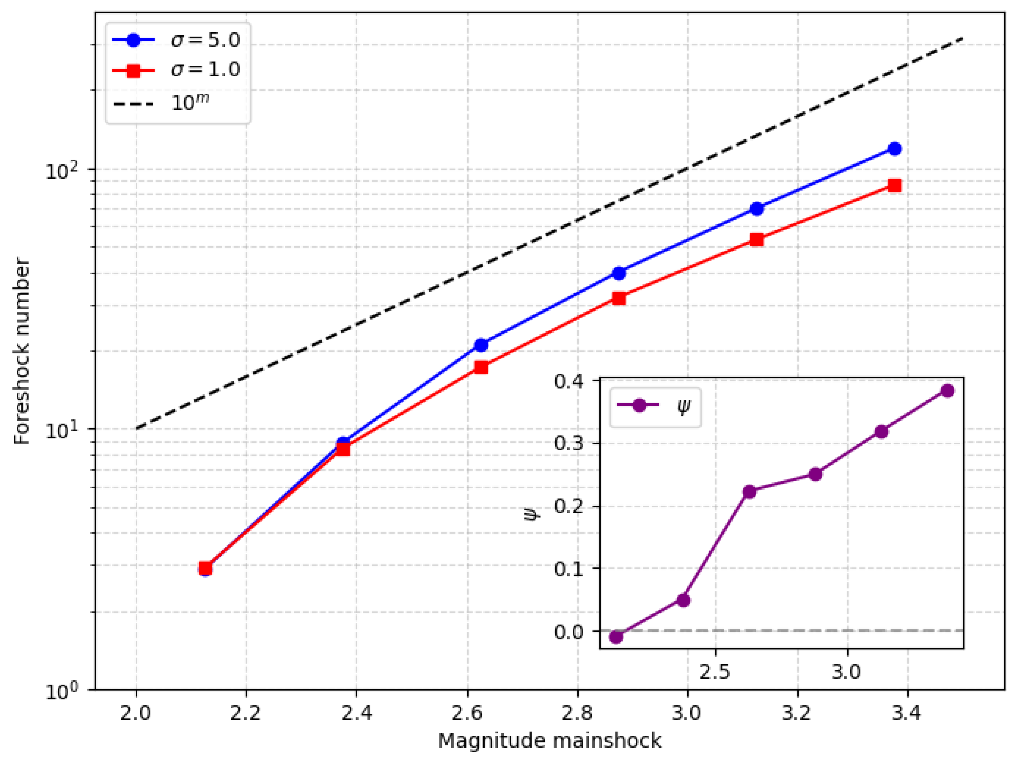
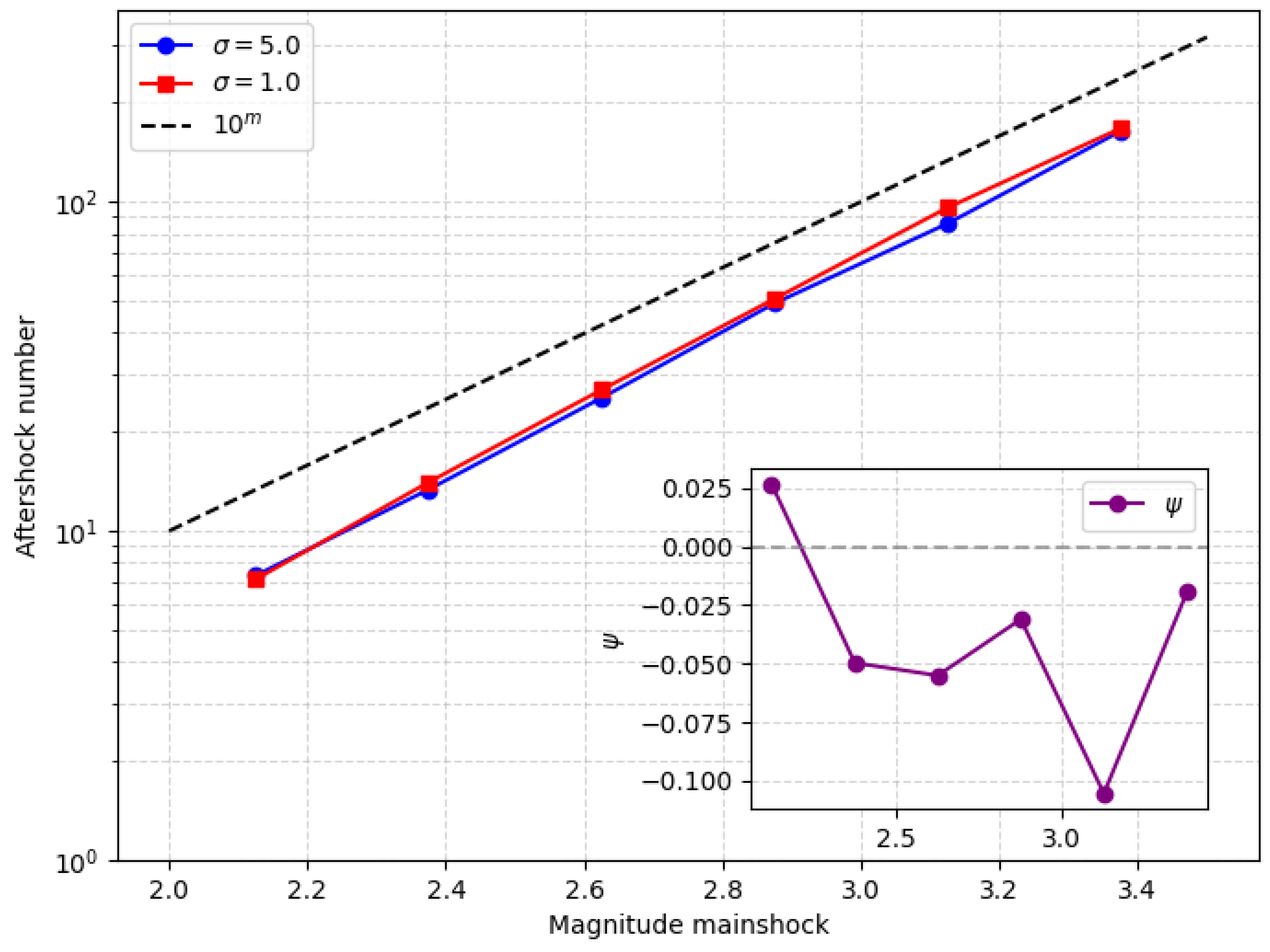
3. Results
4. Discussion
5. Conclusions
Funding
Data Availability Statement
Acknowledgments
Conflicts of Interest
Appendix A
Appendix A.1. Number of Sequences with Foreshocks

Appendix A.2. The Homogeneous Case σ = 0
Appendix A.3. Universality of the Exponent τ = 3/2
- Separation of timescales enforces marginal stability. The tectonic loading is infinitely slow compared to both coseismic slip and viscoelastic relaxation. This hierarchy of timescales forces the system to hover at a marginally stable point: between one avalanche and the next, the stress accumulates until exactly one block reaches its failure threshold. This enforces a branching ratio equal to unity, the hallmark of a critical branching process [37]
- Mapping to a critical branching process or depinning interface. In a critical branching process, each “parent” failure triggers, on average, one “daughter” failure, leading to . Similarly, in elastic interface depinning models with quenched disorder, the avalanche-size distribution near the depinning transition also scales as in any dimension [39].
- Why does not lead to unphysical divergences. A pure power-law with would imply a divergent mean if extended to . However, in any real fault (and in our finite lattice), a natural cutoff limits the maximum avalanche size. Once a slipping region spans the entire lattice, it cannot grow larger. This finite-size cutoff ensures a well-behaved .
Appendix A.4. Algorithmic Description of the Model
- 1.
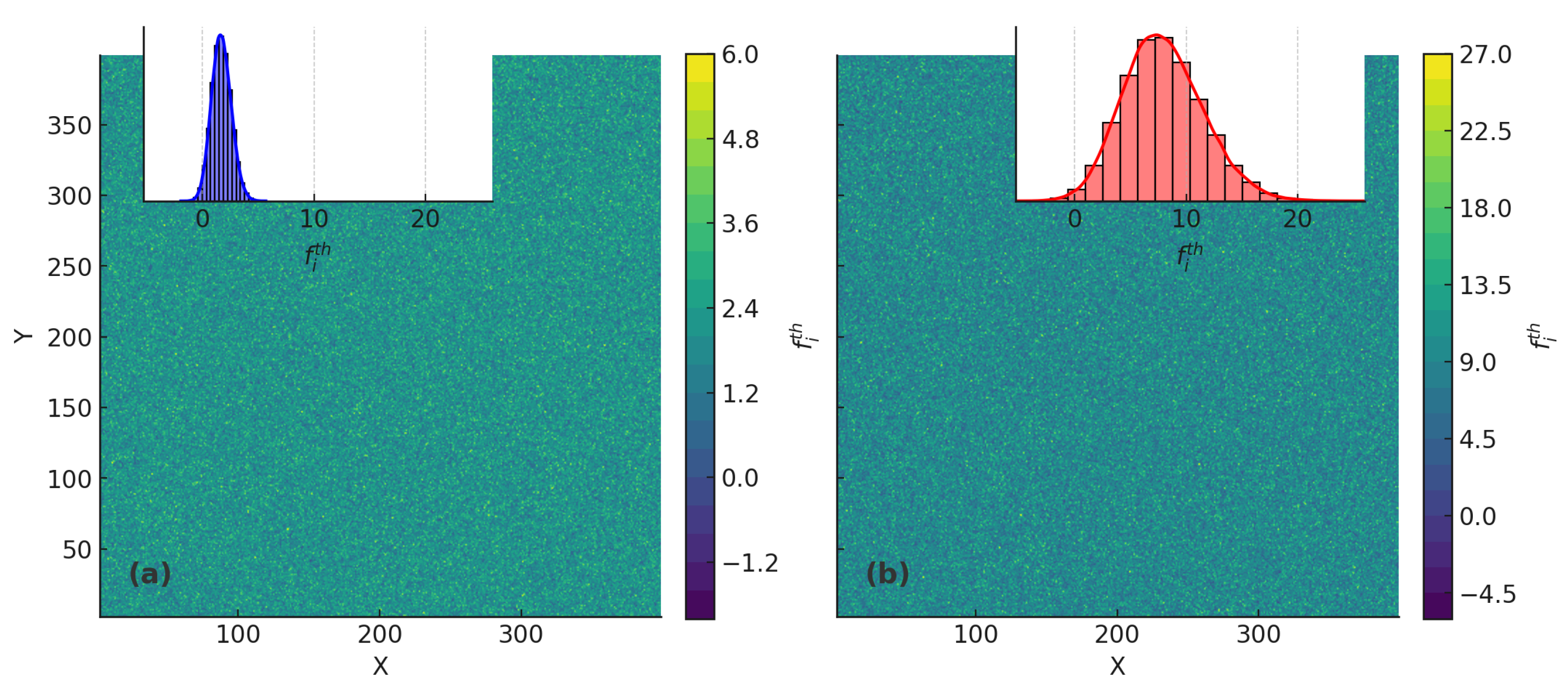
- Initialization. The blocks are initialized with displacements . The failure thresholds are drawn from a Gaussian distribution with mean 1 and variance . The initial stresses are set according to Equation (1).
- 2.
- Driving. The tectonic loading is increased until the most unstable block reaches its threshold, i.e., . The corresponding time increment is .
- 3.
- Avalanche. The block j that reaches the threshold fails, triggering an avalanche:
- The stress is redistributed to neighboring blocks according to Equation (3).
- The block j is assigned a new random threshold .
- If any neighboring block now satisfies , it also fails and the process repeats recursively.
The avalanche continues until all blocks satisfy . - 4.
- Relaxation. After the avalanche, the relaxation function decreases according to a prescribed relaxation law.
- 5.
- Repeat. The system returns to Step 2. The driving continues, and the process repeats to generate the synthetic catalog.
References
- de Arcangelis, L.; Godano, C.; Grasso, J.R.; Lippiello, E. Statistical physics approach to earthquake occurrence and forecasting. Phys. Rep. 2016, 628, 1–91. [Google Scholar] [CrossRef]
- Mignan, A. The debate on the prognostic value of earthquake foreshocks: A meta-analysis. Sci. Rep. 2014, 4, 4099. [Google Scholar] [CrossRef]
- Ogata, Y. Statistical Models for Earthquake Occurrences and Residual Analysis for Point Processes. J. Am. Stat. Assoc. 1988, 83, 9–27. [Google Scholar] [CrossRef]
- Ogata, Y. Statistical model for standard seismicity and detection of anomalies by residual analysis. Tectonophysics 1989, 169, 159–174. [Google Scholar] [CrossRef]
- Petrillo, G.; Zhuang, J. Bayesian earthquake forecasting approach based on the epidemic type aftershock sequence model. Earth Planets Space 2024, 76, 78. [Google Scholar] [CrossRef]
- Petrillo, G.; Lippiello, E.; Zhuang, J. Including stress relaxation in point-process model for seismic occurrence. Geophys. J. Int. 2024, 236, 1332–1341. [Google Scholar] [CrossRef]
- Petrillo, G.; Kumazawa, T.; Napolitano, F.; Capuano, P.; Zhuang, J. Fluids-triggered swarm sequence supported by a nonstationary epidemic-like description of seismicity. Seismol. Res. Lett. 2024, 95, 3207–3220. [Google Scholar] [CrossRef]
- Brodsky, E.E.; Lay, T. Recognizing foreshocks from the 1 April 2014 Chile earthquake. Science 2014, 344, 700–702. [Google Scholar] [CrossRef]
- Petrillo, G.; Lippiello, E. Testing of the foreshock hypothesis within an epidemic like description of seismicity. Geophys. J. Int. 2021, 225, 1236–1257. [Google Scholar] [CrossRef]
- Petrillo, G.; Lippiello, E. Incorporating Foreshocks in an Epidemic-like Description of Seismic Occurrence in Italy. Appl. Sci. 2023, 13, 4891. [Google Scholar] [CrossRef]
- Ogata, Y. Space-Time Point Process Models for Earthquake Occurrences. Ann. Inst. Stat. Math. 1998, 50, 379–402. [Google Scholar] [CrossRef]
- Ogata, Y.; Katsura, K. Comparing foreshock characteristics and foreshock forecasting in observed and simulated earthquake catalogs. J. Geophys. Res. Solid Earth 2014, 119, 8457–8477. [Google Scholar] [CrossRef]
- Zhuang, J.; Ogata, Y.; Vere-Jones, D. Analyzing earthquake clustering features by using stochastic reconstruction. J. Geophys. Res. Solid Earth 2004, 109. [Google Scholar] [CrossRef]
- Liu, Y.; Zhuang, J.; Guo, Y.; Jiang, C.; Tian, Q.; Zhang, Y.; Long, F. Background and clustering characteristics of recent seismicity in Southwestern China. Geophys. J. Int. 2024, 238, 1291–1313. [Google Scholar] [CrossRef]
- Helmstetter, A.; Sornette, D. Foreshocks explained by cascades of triggered seismicity. J. Geophys. Res. Solid Earth 2003, 108. [Google Scholar] [CrossRef]
- Felzer, K.; Abercrombie, R.; Ekstrom, G. A Common Origin for Aftershocks, Foreshocks, and Multiplets. Bull. Seismol. Soc. Am. 2004, 94, 88–98. [Google Scholar] [CrossRef]
- Hardebeck, J.L.; Felzer, K.R.; Michael, A.J. Improved tests reveal that the accelerating moment release hypothesis is statistically insignificant. J. Geophys. Res. Solid Earth 2008, 113. [Google Scholar] [CrossRef]
- Marzocchi, W.; Zhuang, J. Statistics between mainshocks and foreshocks in Italy and Southern California. Geophys. Res. Lett. 2011, 38. [Google Scholar] [CrossRef]
- Spatial organization of foreshocks as a tool to forecast large earthquakes. Sci. Rep. 2012, 2, 846.
- Shearer, P.M. Self-similar earthquake triggering, Båth’s law, and foreshock/aftershock magnitudes: Simulations, theory, and results for southern California. J. Geophys. Res. Solid Earth 2012, 117. [Google Scholar] [CrossRef]
- Seif, S.; Zechar, J.D.; Mignan, A.; Nandan, S.; Wiemer, S. Foreshocks and their potential deviation from general seismicity. Bull. Seismol. Soc. Am. 2019, 109, 1–18. [Google Scholar] [CrossRef]
- Trugman, D.T.; Ross, Z.E. Pervasive foreshock activity across southern California. Geophys. Res. Lett. 2019, 46, 8772–8781. [Google Scholar] [CrossRef]
- Goebel, T.H.; Schuster, V.; Kwiatek, G.; Pandey, K.; Dresen, G. A laboratory perspective on accelerating preparatory processes before earthquakes and implications for foreshock detectability. Nat. Commun. 2024, 15, 5588. [Google Scholar] [CrossRef]
- Perfettini, H.; Avouac, J.P. Postseismic relaxation driven by brittle creep: A possible mechanism to reconcile geodetic measurements and the decay rate of aftershocks, application to the Chi-Chi earthquake, Taiwan. J. Geophys. Res. Solid Earth 2004, 109. [Google Scholar] [CrossRef]
- Petrillo, G.; Lippiello, E.; Landes, F.P.; Rosso, A. The influence of the brittle-ductile transition zone on aftershock and foreshock occurrence. Nat. Commun. 2020, 11, 3010. [Google Scholar] [CrossRef] [PubMed]
- Petrillo, G.; Rosso, A.; Lippiello, E. Testing of the Seismic Gap Hypothesis in a Model With Realistic Earthquake Statistics. J. Geophys. Res. Solid Earth 2022, 127, e2021JB023542. [Google Scholar] [CrossRef]
- Lippiello, E.; Petrillo, G.; Landes, F.; Rosso, A. Fault heterogeneity and the connection between aftershocks and afterslip. Bull. Seismol. Soc. Am. 2019, 109, 1156–1163. [Google Scholar] [CrossRef]
- Lippiello, E.; Petrillo, G.; Landes, F.; Rosso, A. The genesis of aftershocks in spring slider models. Stat. Methods Model. Seism. 2021, 1, 131–151. [Google Scholar]
- Godano, C.; Petrillo, G.; Lippiello, E. Evaluating the incompleteness magnitude using an unbiased estimate of the b value. Geophys. J. Int. 2024, 236, 994–1001. [Google Scholar] [CrossRef]
- Hainzl, S. Rate-dependent incompleteness of earthquake catalogs. Seismol. Res. Lett. 2016, 87, 337–344. [Google Scholar] [CrossRef]
- Cattania, C.; Segall, P. Precursory Slow Slip and Foreshocks on Rough Faults. J. Geophys. Res. Solid Earth 2021, 126, e2020JB020430. [Google Scholar] [CrossRef]
- Ben-Zion, Y.; Zaliapin, I. Localization and coalescence of seismicity before large earthquakes. Geophys. J. Int. 2020, 223, 561–583. [Google Scholar] [CrossRef]
- McLaskey, G.C. Earthquake Initiation From Laboratory Observations and Implications for Foreshocks. J. Geophys. Res. Solid Earth 2019, 124, 12882–12904. [Google Scholar] [CrossRef]
- Papadopoulos, G.; Agalos, A.; Minadakis, G.; Triantafyllou, I.; Krassakis, P. Short-Term Foreshocks as Key Information for Mainshock Timing and Rupture: The Mw6.8 25 October 2018 Zakynthos Earthquake, Hellenic Subduction Zone. Sensors 2020, 20, 5681. [Google Scholar] [CrossRef]
- Im, K.; Avouac, J.P. Cascading foreshocks, aftershocks, and earthquake swarms in a discrete fault network. Geophys. J. Int. 2023, 235, 831–852. [Google Scholar] [CrossRef]
- Lippiello, E.; Petrillo, G. b-more-incomplete and b-more-positive: Insights on a robust estimator of magnitude distribution. J. Geophys. Res. Solid Earth 2024, 129, e2023JB027849. [Google Scholar] [CrossRef]
- Harris, T.E. The Theory of Branching Processes; Springer: Berlin/Heidelberg, Germany, 1963. [Google Scholar]
- Bak, P.; Tang, C.; Wiesenfeld, K. Self-organized criticality: An explanation of 1/f noise. Phys. Rev. Lett. 1987, 59, 381–384. [Google Scholar] [CrossRef]
- Jagla, E.A.; Landes, F.P.; Rosso, A. Viscoelastic effects in avalanche dynamics: A key to earthquake statistics. Phys. Rev. Lett. 2014, 112, 174301. [Google Scholar] [CrossRef]
Disclaimer/Publisher’s Note: The statements, opinions and data contained in all publications are solely those of the individual author(s) and contributor(s) and not of MDPI and/or the editor(s). MDPI and/or the editor(s) disclaim responsibility for any injury to people or property resulting from any ideas, methods, instructions or products referred to in the content. |
© 2025 by the author. Licensee MDPI, Basel, Switzerland. This article is an open access article distributed under the terms and conditions of the Creative Commons Attribution (CC BY) license (https://creativecommons.org/licenses/by/4.0/).
Share and Cite
Petrillo, G. The Role of Disorder in Foreshock Activity. Geosciences 2025, 15, 226. https://doi.org/10.3390/geosciences15060226
Petrillo G. The Role of Disorder in Foreshock Activity. Geosciences. 2025; 15(6):226. https://doi.org/10.3390/geosciences15060226
Chicago/Turabian StylePetrillo, Giuseppe. 2025. "The Role of Disorder in Foreshock Activity" Geosciences 15, no. 6: 226. https://doi.org/10.3390/geosciences15060226
APA StylePetrillo, G. (2025). The Role of Disorder in Foreshock Activity. Geosciences, 15(6), 226. https://doi.org/10.3390/geosciences15060226