Two Opposite Change Patterns Before Small Earthquakes Based on Consecutive Measurements of Hydrogen and Oxygen Isotopes at Two Seismic Monitoring Sites in Northern Beijing, China

Abstract

In comparison with conventional hydrological parameters such as water levels and temperatures, geochemical changes induced by earthquakes have become increasingly important. It should be noted that hydrogen (δ²H) and oxygen isotopes (δ¹⁸O) offer the greatest potential as precursor proxies of earthquakes. Here, we conducted high-resolution sampling (weekly, 59 samples), measuring consecutive δ²H and δ¹⁸O levels at the two sites of the WLY well and SS spring in the Yan-Huai Basin of Beijing from June 2021 to June 2022. During the period of this sampling, several small earthquakes of ML > 1.6 occurred in Beijing. We used statistical methods (analysis of variance) to test the significant differences, used Self-Organizing Maps (SOMs) for data clustering, and then used Bayesian Mixing Models (MixSIAR) to calculate the proportions of the source contributions. We found significant four-stage patterns of change processes in δ²H and δ¹⁸O at both sites. The WLY well exhibited a distinct four-stage variation pattern: initial stable development (WT1) followed by a rapid rise (WT2) and sudden fall (WT3) before the small earthquakes, and finally gradual stabilization after earthquakes (WT4). In contrast, the SS spring displayed an inverse pattern, beginning with stable development (ST1), then undergoing a rapid falling (ST2) and sudden rising (ST3) before the small earthquakes, and finally stabilizing through stepwise reduction after the earthquakes (ST4). The most likely mechanisms were differences in the time of rupture between the carbonate in WLY and granite in SS under sustained stress. The stress induced source mixing of fluid from the surface or deeper groundwater-source reservoirs. The hypothesis was supported by the MixSIAR model, calculating the variational proportion of source contributions in the four stages. This work permitted the use of high-resolution isotopic data for statistical confirmation of concomitant shifts during the earthquakes, provided the mechanisms behind them, and highlighted the potential for the consecutive monitoring of hydrogen and oxygen isotopes indicators in earthquake-prediction studies.

1. Introduction

As part of earthquake precursor detection programs, changes in groundwater levels, temperatures, and chemical parameters related to earthquakes have been documented for decades [1,2,3,4,5,6,7,8,9,10]. In comparison with conventional hydrological parameters such as water levels and temperatures, geochemical changes induced by earthquakes have become increasingly important [4,10,11], because geochemical changes are considered to be sensitive to crustal stress and to be beneficial for earthquake prediction [3,12,13,14,15,16,17,18]. These papers have led to an overall acceptance among scientists that hydrochemical changes could exist following earthquakes and that hydrochemical precursors warrant further investigation (Ingebritsen and Manga, 2014) [18].

From geochemical studies, it should be noted that δ¹⁸O and δ²H offer the greatest potential as precursor proxies of earthquakes [19], able to record the mixing/switching of groundwater sources that have been affected by water–rock interaction. Claesson et al. (2004) [11] observed simultaneous changes in these isotopes before and after major earthquakes. Skelton et al. (2014) [20] observed that δ²H maxima are probable precursors to consecutive earthquakes and performed a statistical evaluation between hydrochemical phenomena and earthquakes. Skelton et al. (2019) [19] found the statistical significance of pre-seismic and post-seismic changes in δ¹⁸O and δ²H in several earthquakes.

In previous studies, we have discussed the characterization of continuous geochemical parameters in response to earthquakes, but we lacked the consecutive δ¹⁸O and δ²H isotope variations at the two sites of WLY well and SS spring in Northern Beijing. For example, Chen and Liu (2023) [21] investigated the sensitivity of trace element constituents in SS spring to small earthquakes, and discussed the mechanisms of the four changed modes in the trace elements. Chen et al. (2024) [22] examined the sensitivity of multiple geochemical parameters of the Wuliying well when responding to small earthquakes, including groundwater level, temperature, major ions, trace elements, and gases, to assess the validity of geochemistry as a monitoring and predictive tool. Furthermore, in these studies, there is a lack of comparison of geochemical characteristics across two sites concerning different tectonic settings, rock types, and the statistical evaluation of the association between geochemical parameters and earthquakes.

Therefore, this paper conducted high-resolution sampling (weekly, 59 samples per site), measuring consecutive hydrogen (δ²H) and oxygen isotope (δ¹⁸O) levels at two sites in Northern Beijing from June 2021 to June 2022. Statistical analysis was adopted to test the significant differences among the stages of data variation, while Self-Organizing Maps (SOMs) were used for data clustering, and Bayesian Mixing Models were used for calculating the proportions of different source contributions to the mixture. Finally, this paper discusses the mechanism of isotope change patterns before earthquakes.

2. Background

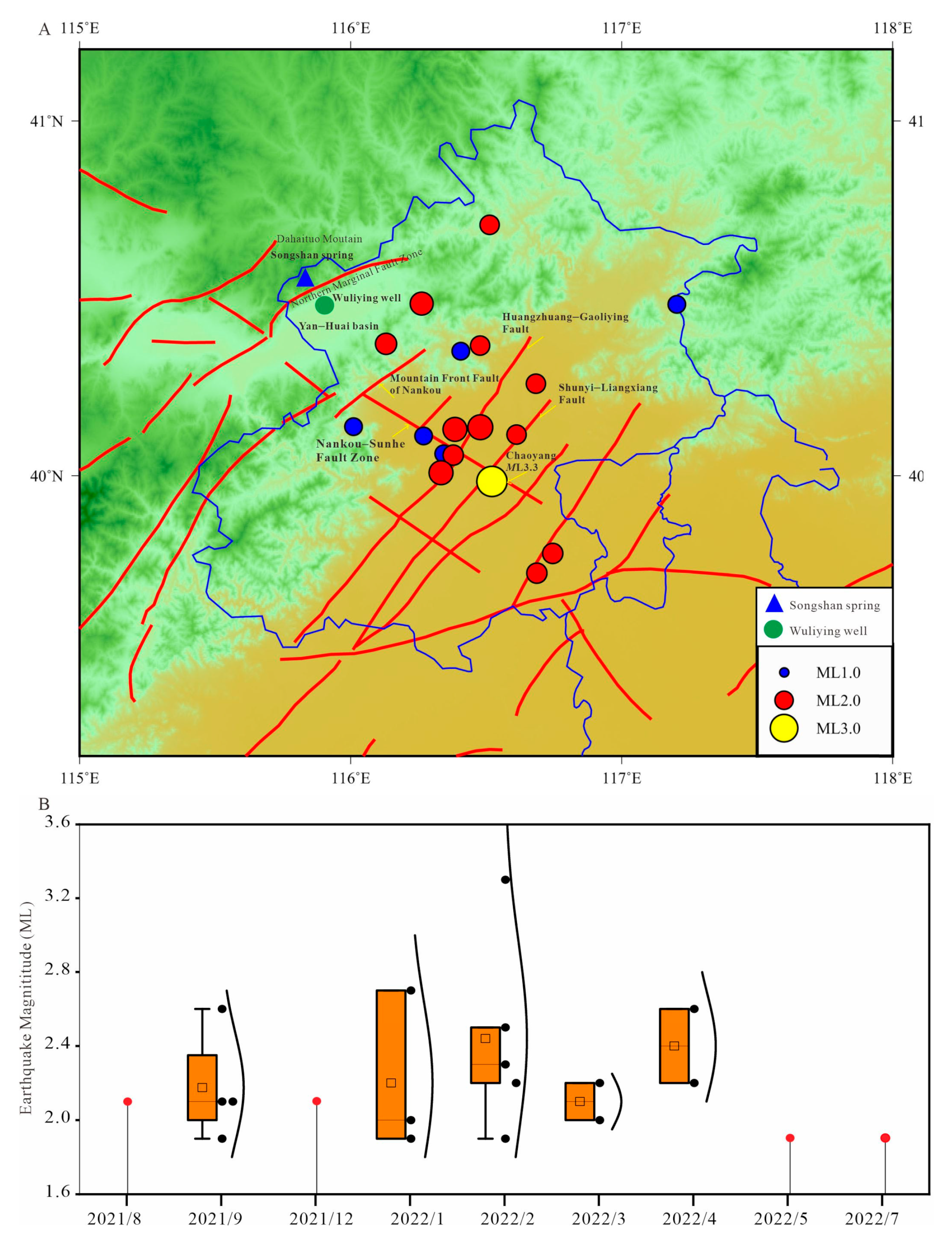
2.1. Faults and Earthquakes in Beijing

Beijing is the capital of China, with a large population. It is located in the intersection of the North China Plain and Zhang-Bo (Zhangjiakou-Bohai) seismic belt.

Beijing has also developed regional active faults, mainly including the NW-orderly Nankou–Sunhe Fault Zone and two groups of NE-orderly active fault zones named the Huangzhuang–Gaoliying Fault Zone and Shunyi–Liangxiang Fault Zone (Figure 1). All earthquakes in Beijing occur along these fault zones or where they intersect (Figure 1), and almost all of these earthquakes are less than M3. Therefore, there is great scientific and practical significance to small earthquake monitoring and prediction in the Beijing area.

Beijing hosted the 2022 Winter Olympic Games from 4 to 20 February. For security purposes, the continuous monitoring of possible earthquake areas was strengthened. During the research period, about 400 earthquakes were recorded in Beijing (Figure 1A), only 20 of which were above ML1.6. On 3 February 2022, the biggest earthquake, with a magnitude of ML3.3, occurred in the Chaoyang District of Beijing (Figure 1). Furthermore, eight earthquakes above M1.5 occurred densely during January to February 2022 (Figure 1B).

2.2. Hydrological Conditions

The Wuliying (WLY) well is located in the north of Wuliying village in the Yanqing District of Beijing. The well is 2 km west of the Yanqing seismic monitoring station, and has an epicentral distance of ~65 km from the Chaoyang earthquake (Figure 1). Geologically, the Wuliying well is located in the Yan-Huai (Yanqing-Huailai) sediment Basin, the junction area of Yanshan Mountain and the Zhang-Bo seismic belt. The Northern Marginal Fault Zone of the Yan-Huai Basin is 3 km northwest of the well, and pressure faults developed around the well area, so the structural site of the well is sensitive to stress changes.

The Wuliying well was drilled in 1984 with a depth of 533 m; its lithology consists of Quaternary sediment, Jurassic basalt, and Sinian (Pre-Cambrian) carbonate (limestone and dolostone); the wellbore is open to Pre-Cambrian carbonate from 505 m to the bottom of the well [22]. The well is a flowing artesian geothermal well with a flow rate of 2.5 L/s, temperature of 33.4 °C, pH of 7.3, and a water type of HCO₃-Na [22]. Multiple geochemical parameters of WLY well have been reported in detail by [22], including daily measured water level, water temperature, four major ions (F⁻, Cl⁻, SO₄²⁻, NO₃⁻), five dissolved gases in the water (Hg, H₂, He, N₂, CH₄), and three degassing gases (Hg, Rn, H₂). This sufficient data provided an important foundation for earthquake monitoring and prediction in Beijing.

The Songshan (SS) hot spring is ~10 km away from the Wuliying well. The spring is of an artesian geothermal type, and its water source is from the granite rock body of Dahaituo Mountain, which is also near the Northern Marginal Fault of the Yan-Huai Basin (Figure 1). The investigation of trace elements in Songshan Spring was first documented in detail by [21].

3. Material and Methods

3.1. Data Collection

Water samples were collected (total of 59 per site) with relatively high sample rates (every 7–10 days) for hydrogen (δ²H) and oxygen isotopic (δ¹⁸O) analysis from June 2021 to July 2022 in WLY, and from August 2021 to August 2022 in SS, respectively. The sampling and analytical procedures have been described by Chen and Liu (2023) [21]: Each sample was stored in a 200 mL polyethylene bottle. All samples were sent monthly to the Beijing Earthquake Agency for hydrogen and oxygen isotopic analysis with Picarro liquid water and a water vapor isotope analyzer with an accuracy of 0.2‰ for δ¹⁸O and δ²H. All geochemical results are listed in Table S1.

Laboratory quality-assurance and quality-control methods were used to ensure the quality of the analytical data, including standard calibration, the use of standard operating procedures, and reagent blank analysis. All analyses were performed in triplicate. Reagent blanks were monitored throughout analysis and used to correct analysis results.

3.2. Analytical Methods

Statistical analysis was conducted (ANOVA test) in Past version 4.04 software [23,24] to permit statistical verification among different stages of data variation, Self-Organizing Maps (SOMs) were used for data clustering, and then a Bayesian mixing model (MixSIAR version 3.1.9) was used in the R program version 4.4.2 for calculating the proportions of the source contributions to a mixture.

The ANOVA test (analysis of variance) is a statistical procedure for testing the null hypothesis that several univariate samples are taken from populations with the same mean. The samples were assumed to be close to normally distributed and have similar variances. Thus, the ANOVA test was used to analyze the differences among group means in a sample. If the ANOVA showed significant inequality between the means (small p), the given table of post hoc pairwise comparisons would be further studied, based on the Tukey–Kramer test. The difference among the groups in isotopic data was considered statistically significant if the p value obtained using this test was less than 0.05.

$$\mathrm{Q}={\displaystyle \frac{XL-XS}{\sqrt{\frac{M}{n}}}}$$

XL is the larger and XS the smaller mean of the two samples being compared. If the two sample sizes are not equal, their harmonic mean is used for n. Its significance is estimated according to [25].

The Self-Organizing Maps (SOMs) model is an unsupervised artificial neural network model. Ref. [26] proposed the SOMs algorithm and introduced its specific implementation process. This method simulates the biological brain’s learning process to make a cluster area form near each best-matching neuron so that the input vectors of similar features are classified into a cluster. At the same time, SOMs provide a visualization method for high-dimensional data projection in low-dimensional space, such as two-dimensional space, while retaining the topological structure and metric relationships of the original data [27], which is suitable for high-dimensional data reduction, classification, and visualization. Heuristic rules can be used to select the appropriate number of neurons, such as 5× sqrt (n), as suggested by [27], where n is the number of samples. The K-means algorithms, which are the most popular and straightforward clustering algorithms, are frequently applied for efficient clustering due to their implementation simplicity and low computational complexity [28,29]. In this study, the SOMs algorithm toolbox was implemented by MATLAB version 2018 software according to the method described by [27], and then the K-means clustering algorithm was run, based on the results from the SOM, to determine the optimal number of clusters.

A Bayesian isotope mixing model (MixSIAR) was proposed by [30]. The model uses a Bayesian framework to determine the probability distribution of contributions from each source while fully accounting for uncertainties associated with multiple sources, fractionation effects, and isotopic signatures. A new Bayesian isotope mixing model, MixSIAR, combines the strengths of the former Bayesian model and has been widely used in the identification of groundwater source contributions [31]. By considering the source values, the MixSIAR model has improved upon the simpler linear mixing model, as was expressed by [32].

4. Results

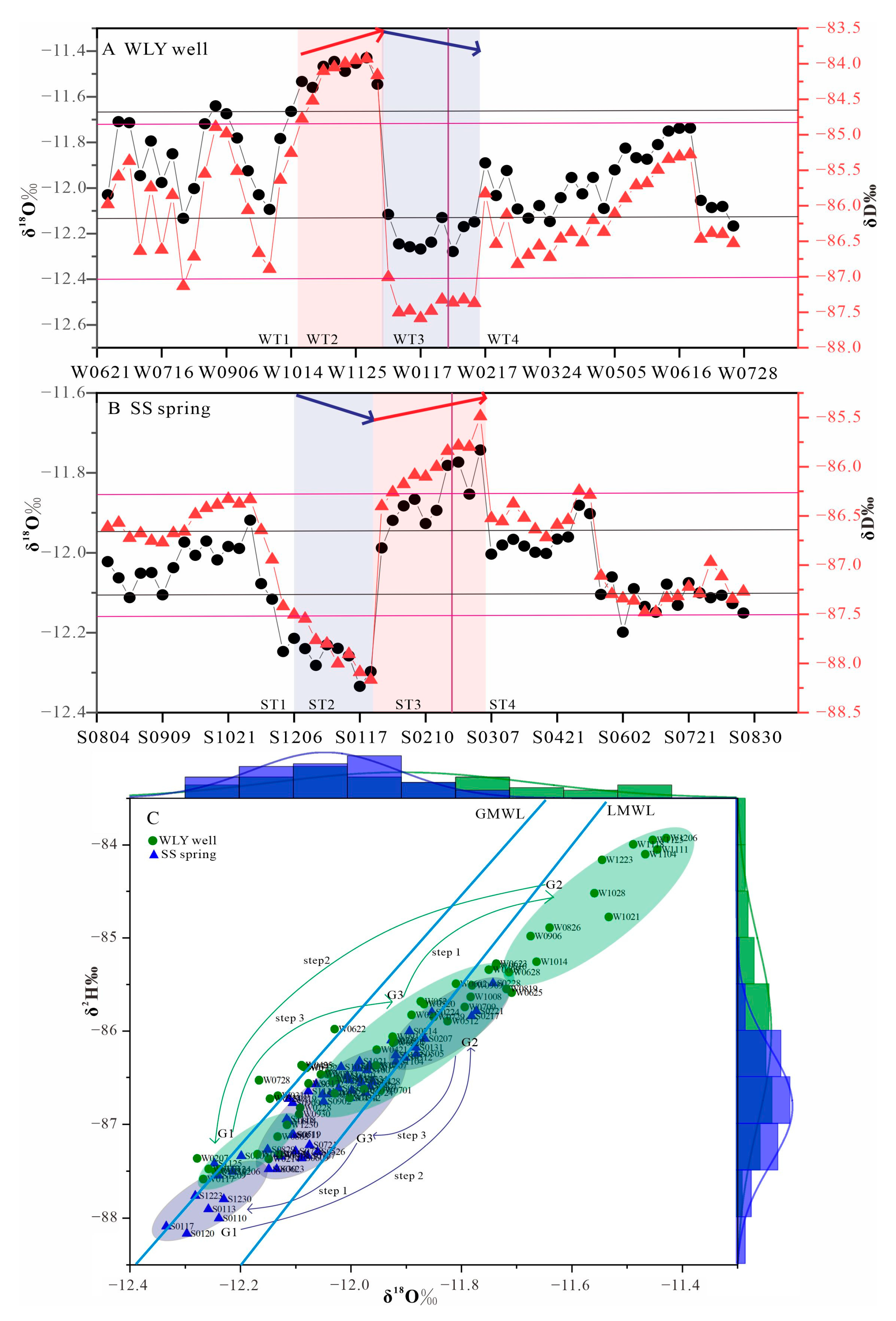
4.1. Time Series Characteristics

In this study, obvious stepwise shifts of δ²H and δ¹⁸O were observed over the time sequence. There are four distinct stages in both WLY (WT1, WT2, WT3, WT4) and SS (ST1, ST2, ST3, ST4) by time sequence during sampling. At the Wuliying well, isotopes firstly had stable development (WT1), then a rapid rise (WT2), followed by a sudden fall (WT3), and finally a gradual rise recovery (WT4). The SS data show opposite change patterns by time series. At the SS spring, isotopes also firstly had stable development (ST1), then rapid fall (ST2), a sudden rise (ST3), and finally a stepwise reduction stabilization (ST4). The detailed descriptions of each phase are as follows:

At Wuliying well, oxygen isotopes had four distinct stages (Figure 2A) in the order of the time series: In the first stage (WT1), oxygen isotopes changed between −12.1‰ and −11.7‰ from June to September 2021. In the second stage (WT2), the oxygen isotope values were highest, all above −11.7‰ from October to November 2021. In the third stage (WT3), the oxygen isotope values were lowest, all below −12.1‰ from December 2021 to January 2022. In the fourth stage (WT4), oxygen isotope levels gradually increased from −12.1‰ to −11.7‰ from February to July 2022. The hydrogen isotopes show the same trend as oxygen (Figure 2A): In WT1, hydrogen isotopes changed between −87‰ and −84.7‰. In WT2, the hydrogen isotope values peaked, all above −84.7‰. In WT3, the hydrogen isotope values were at their lowest, all below −87‰. In WT4, the hydrogen isotopes also gradually increased from −87‰ and −84.7‰. The isotopes in WLY have a change pattern of stable development (WT1), then a rapid rise (WT2), sudden fall (WT3), and finally a gradually increasing stabilization (WT3).

At SS spring, oxygen isotopes also had four obvious stages (Figure 2B) in the order of the time series, with the change trend in SS opposite to in WLY: In the first stage (ST1), the oxygen isotopes changed between −12.15‰ and −11.95‰ from August to November 2021. In the second stage (ST2), the oxygen isotope values were at their lowest, all below −12.15‰ from December 2021 to early January 2022. In the third stage (ST3), the oxygen isotope values were the highest, all above −11.95‰ from early January to February 2022. In the fourth stage (ST4), the oxygen isotope values fluctuated around −11.95‰ from March to May 2022 and then fluctuated around −12.15‰ from June to August 2022. The hydrogen isotopes have a very similar trend to oxygen (Figure 2B): In ST1, the hydrogen isotopes changed between −87.5‰ and −86.3‰. In ST2, the hydrogen isotope values were the lowest, all below −87.5‰. In ST3, the hydrogen isotope values were the highest, all above −86.3‰. In ST4, the hydrogen isotope values fluctuated around −86.3‰ from March to May 2022 and then fluctuated around −87.5‰ from June to August 2022. So, the isotopes in SS showed a change pattern of stable development (ST1), then a rapid fall (ST2), sudden rise (ST3), and finally a stepwise reduction stabilization (ST4).

The data shows that the δ¹⁸O and δ²H values at the WLY well and SS spring were distributed mainly along the GMWL (global meteoric water line, from [33]) and LMWL (local meteoric water line, from [34]). These values straddle both the GMWL and IMWL, and can be roughly classified into three groups based on their distribution shown in Figure 2C: The first group (G1) is distributed in the lower left corner of the figure: the δ²H and δ¹⁸O values are the most negative, ranging from −87.6‰ to −87‰ and from −12.3‰ to −12.1‰ in the WLY well (green oval-shaped area). The δ²H and δ¹⁸O values range from −88.5‰ to −87.5‰ and from −12.35‰ to −12.15‰ in the SS spring (blue oval-shaped area). The first group was most likely affected by deep geological effects, such as deeper groundwater mixing. The second group (G2) is distributed in the upper right corner of the figure: the δ²H and δ¹⁸O values are the most positive, ranging from −85.5‰ to −84.5‰ and from −11.7‰ to −11.4‰ in the WLY well (green oval-shaped area). The δ²H and δ¹⁸O values range from −86.5‰ to −85.5‰ and from −11.9‰ to −11.7‰ in the SS spring (blue oval-shaped area). The second group was most likely affected by surface water effects, maybe mixing with atmospheric precipitation or surface water (river water). It should be noted that the samples in the second group trended to the right of the GMWL/LMWL, indicating the strengthened degrees of water–rock interaction. The third group (G3) is distributed in the middle part, above the other two groups: the δ²H and δ¹⁸O values range relatively widely from −87‰ to −85.5‰ and from −12.1‰ to −11.7‰ in the WLY well (green oval-shaped area). The δ²H and δ¹⁸O values range from −87.5‰ to −86.3‰ and from −12.15‰ to −11.9‰ in the SS spring (blue oval-shaped area).

These three groups (G1, G2, G3) based on the distribution in the bivariant plots of δ²H-δ¹⁸O correspond well to the previous four stages (T1, T2, T3, T4) organized by time sequence. In the WLY pattern, G3-G2-G1-G3 match to WT1-WT2-WT3-WT4, with G2 corresponding to WT2, G1 corresponding to WT3, and G3 including WT1 and WT4. In the SS pattern, G3-G1-G2-G3 match to ST1-ST2-ST3-ST4, with G1 corresponding to ST2, G2 corresponding to ST3, and G3 including ST1 and ST4. WLY has a pattern of change that shows stable development, with an initial rise, then a fall, and finally a gradual rising recovery, as shown (Figure 2C): the levels quickly jump from Group 3 to Group 2 in step 1, then quickly decrease to Group 1 in step 2, finally gradually rising back up to Group 1. The simple summary is G3-G2-G1-G3. Notably, SS shows a pattern of stable development, falling first, then rising, with a final gradual rising recovery, as shown: the levels quickly jump down from Group 3 to Group 1 in step 1, then quickly increase to Group 2 in step 2, and finally gradually decline back to Group 1. The brief summary is G3-G1-G2-G3.

4.2. ANOVA Analysis

To determine if such pre- and post-seismic changes were significant, an ANOVA analysis was conducted for each stage. By dividing the pre-seismic (T1, T2, T3) and post-seismic (T4) stages of the hydrogen and oxygen isotopes, univariate ANOVA analyses could be performed. The results showed that the p values of all the pre-seismic stages were less than 0.05, which was strongly significant (Figure 3). This supported the four stages of data that were statistically separable with respect to δ¹⁸O and δ²H.

In detail, the probability p values of the δ¹⁸O and δ²H at WLY are less than 0.05 among T1, T2, and T3 (Figure 3A,B), which means that the differences among the pre-seismic stages are real according to the statistical test. Notably, the p value of δ¹⁸O between T1 and T4 is 0.037; the p is close to 0.05, so the difference between T1 and T4 is not very significant, which supports the interpretation that the δ¹⁸O at T4 (post-seismic) recovered closely to T1 (pre-seismic) levels. The p value of δD between T1 and T4 is 0.054. The p is above 0.05; thus, the difference between T1 and T4 is not statistically significant, which also supports the interpretation that the δD at T4 (post-seismic) had recovered to the same level as in T1 (pre-seismic).

The probability p values of δ¹⁸O and δ²H at SS are also less than 0.005 among T1, T2, and T3 (Figure 3C,D), which means that the differences among the pre-seismic stages are real. Notably, the p value of δ¹⁸O between T1 and T4 is 0.78, which is obviously above 0.05; thus, the difference between T1 and T4 is not significant, which also supports the interpretation that the δ¹⁸O at T4 (post-seismic) had recovered to same levels as at T1 (pre-seismic). The p value of δ²H between T1 and T4 is 0.004, which is below 0.05, so the δD at T4 (post-seismic) had not recovered to T1 (pre-seismic) levels. Since further long-term post-seismic data have not yet been obtained, the whole post-seismic recovery is difficult to recognize.

5. Discussion

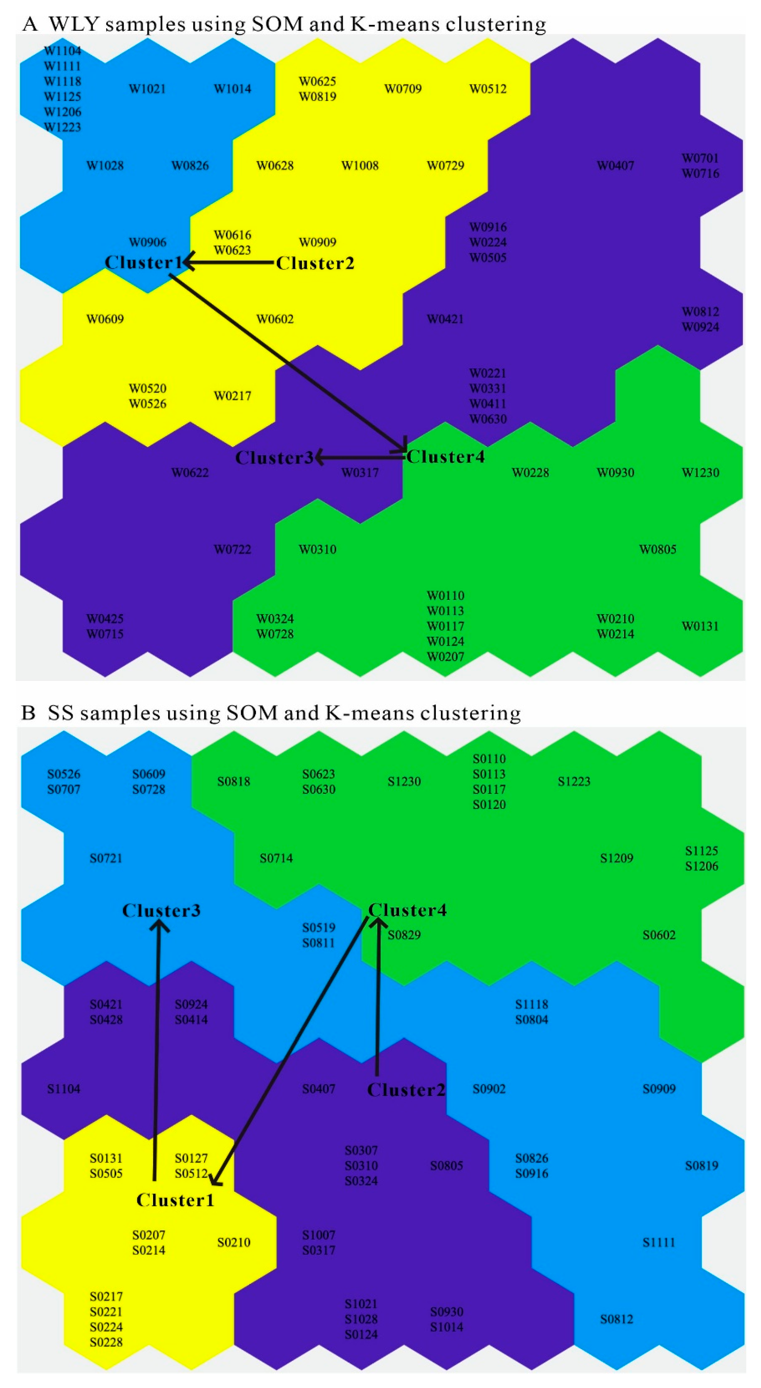
5.1. Self-Organizing Map (SOM) and K-Means Clustering Algorithms

Self-Organizing Maps (SOMs) are a critical branch of artificial neural networks which can map high-dimensional data to low-dimensional space so that some similar properties behave as in geometric neighbor mapping [27]. This indicates that SOM is well suited to clustering analysis and data visualization [35]. In this work, SOMs and K-means clustering is used for δ²H and δ¹⁸O analysis on a temporal scale in the WLY well and SS spring during the study periods (n = 59), so sixty-four (8 × 8) output neurons are selected, and all samples can be categorized into four clusters (Figure 4), distributed along the diagonal.

In the pattern of the WLY cluster, Cluster1 occupies the upper left corner of Figure 4A (blue color), Cluster2 is next to Cluster1, occupying the middle part of the figure (yellow color), Cluster3 (purple color) is adjacent to Cluster2, and Cluster4 occupies the lower right corner of Figure 4A (green color). The Cluster1 mainly contains samples W1014–W1223, which correspond well to the WT2 stage. Cluster2 mainly contains samples W0625–W0909, corresponding to the WT1 stage. The Cluster3 mainly contains samples W0317–W0728, corresponding to the WT4 stage. The Cluster4 mainly contains samples W1230–W0310, corresponding to the WT3 stage. Therefore, in terms of the order of time evolution, the clustering order of WLY should be as follows: Cluster2–Cluster1–Cluster4–Cluster3. The SOM algorithm distinguished well among the pre-earthquake stages and the post-earthquake one at the WLY well.

In the pattern of the SS cluster, Cluster1 occupies the lower left corner of Figure 4B (yellow color), Cluster2 is next to Cluster1, occupying the middle part of the figure (purple color), Cluster3 (blue color) is adjacent to Cluster2, and Cluster4 occupies the upper right corner of Figure 4B (green color). Cluster1 mainly contains samples S0127-S0228, which correspond well to the ST3 stage. The Cluster2 mainly contains samples S0805-S1028, corresponding to the ST1 stage. The Cluster3 mainly contains samples S0519-S0826, corresponding to the ST4 stage. The Cluster4 mainly contains samples S1209-S0120, corresponding to the ST2 stage. Therefore, in terms of the order of time evolution, the clustering order of SS should be as follows: Cluster2–Cluster4–Cluster1–Cluster3. The SOM algorithm also distinguished well among the pre-earthquake stages and the post-earthquake one at SS spring.

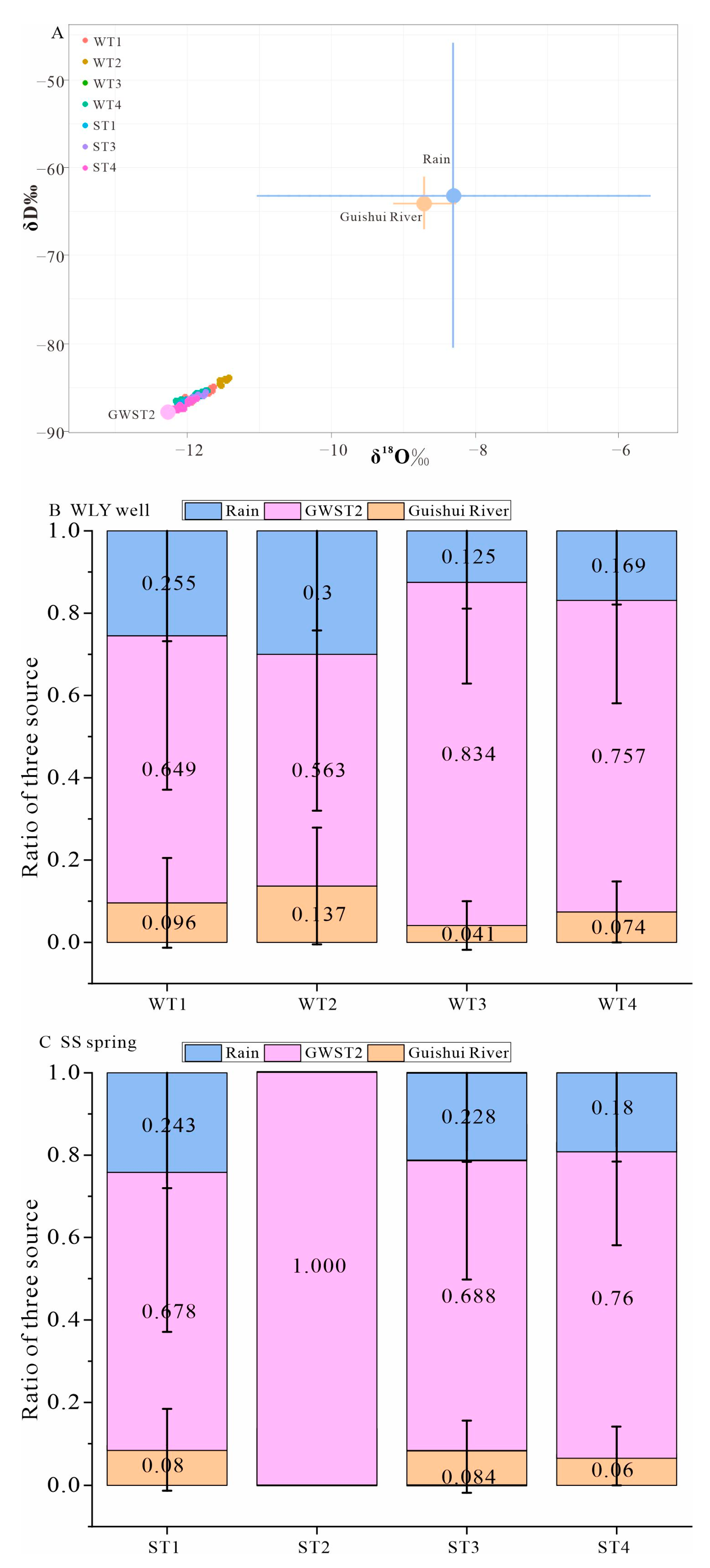
5.2. Quantification of Groundwater Sources

Broadly speaking, hydrogen (δ²H) and oxygen (δ¹⁸O) isotopes are appropriate tracers, and they are extensively used to study the circulation of natural water [33]. The analysis method mainly uses the relationship between groundwater samples and the meteoric water line to discern the source and recharge processes of groundwater, then analyzing whether the groundwater is mixed with the shallow surface water or by a deep source [19,20]. Pre-Holocene groundwater is characterized by δ²H values that are considerably more negative than can be attributed to present-day precipitation [20]. Water–rock interaction has also been inferred based on observations of a shift from the global meteoric water line (GMWL) towards less negative δ¹⁸O values. Specifically, variation in δ²H in groundwater records mixing and/or switching between different groundwater sources, whereas variation in δ¹⁸O in groundwater records water–rock interactions, with rocks only explaining δ¹⁸O shifts towards less negative values [20]. This is because rocks, compared with water, contain proportionally more oxygen than hydrogen [36]. Hence, groundwater δ¹⁸O values are strongly affected by water–rock interaction, while δ²H values are largely unaffected by water–rock interaction and can therefore provide a faithful record of mixing and/or switching between different groundwater sources [20].

Broadly speaking, gradual changes record water–rock interaction or the slow mixing of groundwater sources, reflecting, for example, slow leakage along a fracture system, whereas abrupt changes record switching between sources, reflecting, for example, a sudden rupture of a hydrological barrier between sources [17,20]. Claesson et al. (2004) [11] also attributed sudden geochemical changes to the rupture of a hydrological barrier and opening of a fracture pathway between previously disconnected and chemically distinct groundwater sources. In this study, δ²H and δ¹⁸O isotope changes were dominated by abrupt shifts, reflecting the rapid mixing of previously disconnected water sources.

For determining groundwater origin, the proportional contributions of δ²H and δ¹⁸O sources were evaluated using MixSIAR. The MixSIAR model has been widely used in aqueous isotope source studies, but few have reported on its application in the study of the association between groundwater sources and seismic activities.

Different water sources exhibit distinct isotopic signatures, which can be categorized into the following end-members: 1. The precipitation end-member (atmospheric water), the δ¹⁸O and δ²H values close to the local meteoric water line (LMWL). 2. The surface water end-member (river/lake Water), which deviates from the meteoric water line, showing simultaneous enrichment in δ¹⁸O and δ²H. 3. Paleowater/geothermal water, where the δ¹⁸O and δ²H deviate from modern precipitation, often being more negative. There are other end-member waters that have little to do with this research, including seawater, glacial/snowmelt water, and biologically modified water. Therefore, in this paper, local rain was used to represent the precipitation end-member, the Guishui river represented the local surface water end-member, and GWST2 represented the paleowater/geothermal end-member.

For this purpose, δ²H and δ¹⁸O isotope values were collected for the three potential sources (Figure 5A): Firstly, the atmospheric precipitation source (local rain, mean = −63.2‰, SD = 17.3‰ of δ²H; mean = −8.3‰, SD = 2.7‰ of δ¹⁸O; cited from [37]). Secondly, the local surface source (Guishui river, mean = −64.05‰, SD = 2.98‰ of δ²H; mean = −8.7‰, SD = 0.44‰ of δ¹⁸; cited from [38]). Thirdly, the paleowater/geothermal end-member (local deeper groundwater source) was characterized by more negative hydrogen and oxygen isotopes. However, there are no lower δ²H levels in the documented deeper groundwater than the groundwater of ST2 (GWST2, the T2 stage of SS groundwater) in the Beijing area, so the GWST2 values were used to represent the paleowater/geothermal end-member.

The MixSIAR model indicated potential source contributions of δ²H and δ¹⁸O isotopes (Figure 5). As shown for the WLY well (Figure 5B), the main source was GWST2 (deeper groundwater), and ratios changed over time. Its contribution ranged from 64.9% at WT1 to 56.3% at WT2, 83.4% at WT3, and finally to 75.7% at WT4. Because GWST2 means more negative hydrogen and oxygen isotopes, an increase in the GWST2 ratios means a decrease in the hydrogen–oxygen isotope value. Hence, the changed ratios of GWST2 correspond well to the variation pattern of WLY, that is, first a rise, then a fall, and finally a gradually increasing stabilization.

The main source of SS also was GWST2, as shown in the SS spring (Figure 5C). Its contribution ranged from 67.8% at ST1 to 100% at ST2, 68.8% at ST3, and finally 76.0% at ST4. Because GWST2 means more negative hydrogen and oxygen isotopes, these values also correspond well to the variation stages at SS, falling first and then rising, with a final stepwise reduction stabilization.

5.3. Relationship Between Isotopes Changes and Seismic Activities

There were about 400 earthquakes occurring in the Beijing area during the period of this sampling (from June 2021 to August 2022); only 20 of them were above ML1.6 (Figure 1). On 3 February 2022, the biggest earthquake, with a magnitude of ML3.3, occurred in the Chaoyang District of Beijing (Figure 1). The spatial distribution of these earthquakes spread along the NW-orderly Nankou–Sunhe Fault which was controlled by the large-scale Zhangjiakou-Bohai (Zhang-Bo) Fault Zone in the northwest direction. The WLY and SS sites both correlated with this seismic distribution direction. On a regional scale, there were three earthquakes above M1.0 during the period of this sampling in the Yanqing District, which occurred near the Mountain Front Fault of Nankou (Figure 1), close to the two monitoring sites, so they had a strong spatial correlation.

From a time series perspective, isotopes of the two sites had strong temporal relationships with the small earthquakes. There were eight earthquakes above ML1.6 that densely occurred from January to February 2022 (Figure 1, Supplementary Materials). Seismic activities were relatively intensive from January to February, and the isotopes had statistically significant changes before the small earthquake swarm (before the end of February, Figure 1, Supplementary Materials). Specifically, the isotopes at WLY rapidly increased and exceeded peaks at ±−11.5‰ of δ¹⁸O and ±−84.0‰ of δ²H 105 days before the earthquakes (WT2), then abruptly decreased to their lowest values at ±−12.3‰ of δ¹⁸O and ±−87.5‰ of δ²H 45 days before the earthquakes (WT3), and finally the isotopes gradually rose and returned to their of initial values (WT4) after the earthquakes.

The SS values have opposite change patterns to WLY. The isotopes at SS rapidly decreased to their lowest values at ±−12.3‰ of δ¹⁸O and ±−88.3‰ of δ²H 100 days before the earthquakes (ST2), then abruptly increased to peaks at ±−11.8‰ of δ¹⁸O and ±−86.0‰ of δ²H 35 days before the earthquakes (ST3), abruptly decreased to an average baseline of ±−12.0‰ of δ¹⁸O and ±−86.5‰ of δ²H 75 days after the earthquakes (ST4), then finally abruptly decreased again to an average baseline of ±−12.1‰ of δ¹⁸O and ±−87.3‰ of δ²H 75–100 days after the earthquakes (ST4). In brief, WLY had a change pattern of an initial rise and then a fall before the earthquakes, while SS had a change pattern of an initial fall and then a rise before the earthquakes.

In summary, this coincidence in timing on the two sites is proof of an association with the earthquakes instead of the changes having occurred randomly. Moreover, each significant change at the two sites began about 100 days (14 weeks/three months, and 75 km) before the earthquakes. These time and length scales of seismic–hydrological coupling are broadly consistent with precursory seismic wave propagation anomalies, and the results of other hydrogeochemical studies [19,39] may yield information about the fluid flux rate and/or volume of the stressed region. The statistically significant δ²H and δ¹⁸O isotope anomalies before the small earthquakes highlight the potential importance of stable isotopes as indicators in earthquake-prediction studies.

5.4. Mechanism Analysis

As for the mechanism causing the two opposite change patterns in the isotopes at the two sites before the small earthquake swarm (Supplementary Materials), no correlation between precipitation data and isotope change was observed because seasonal rainfall in Beijing is almost entirely concentrated in rainfall time (June and July each year), and during rainfall time, the δ²H and δ¹⁸O isotopes were stable, with no apparent trend change (Figure 2A,B). In terms of spatial distance, WLY and SS are both located within the region where, based on seismic energy density as an empirical metric, pre-seismic/co-seismic hydrological responses might occur in response to strain associated with small earthquakes (e > 10⁻⁴ J/m³; [21]; methods cited by [9]). Furthermore, it should be noted that the hydrogeological conditions of the aquifer are different at the two sites. The groundwater at SS belonged to bedrock fissure water, with a large burial depth and good closure, which showed relatively low values of hydrogen and oxygen isotopes. The WLY aquifer system was similarly derived from bedrock fissure water. However, its overlying Quaternary sedimentary layer, characterized by significant thickness and abundant sediment pore water, likely facilitated mixing with rainfall and surface water. This hydrological interaction corresponds with the observed elevated hydrogen and oxygen isotopes values in the system.

For the above reasons, this study proposes that the two opposite change patterns were most likely the result of stress on the different rock types of the aquifer. Laboratory studies of rock deformation show that, beyond the elastic limit, the shearing of consolidated rock creates microcracks [40]. At still higher deviatoric stresses, microcracks merge, leading to eventual large-scale rupture [41]. Thus, the differences in the time of rupture between carbonate and granite under sustained stress probably led to opposite patterns in isotopic changes (Figure 6). The aquifer at WLY is made of Pre-Cambrian carbonate (limestone and dolostone), while the bedrock of SS is made of the granite of Dahaituo Mountain. Granite is harder to rupture with stress than carbonates according to rock mechanics experiments [42,43,44]. We inferred that the most likely scenario was that, as the pre-seismic regional stresses started to load (T2 stage from Figure 6), the carbonate rocks of the WLY aquifer were the first to form microfractures, enhancing water–rock interaction, causing the increased δ¹⁸O and sudden influx of surface water/overlying sediment pore water mixing, resulting in peaks in δ²H values. This interpretation is supported by the above MixSIAR model, showing a progressive increase in the proportion of surface water. The contribution source of the Guishui river increased the ranges from 9.6% at T1 to 13.7% at T2 (Figure 5B), and the rain increased from 25.5% at T1 to 30.0% at T2 (Figure 5B). At the same time, the granites of the SS aquifer were not fractured, and deeper groundwater (with more negative hydrogen and oxygen isotopes) was most likely squeezed into the water column, resulting in lower isotope values [20].

As the stress continued to load (T3 from Figure 6), the fractures at WLY exhibited limited development or partial healing [19,45,46,47]. This process weakened water–rock interaction, causing δ¹⁸O depletion, and potentially facilitated the influx of deeper groundwater into the water column, resulting in an abrupt δ²H decrease. The MixSIAR model also verified this hypothesis, identifying the main source contribution of GWST2 (deeper groundwater). Its proportional contribution exhibited an increase from 56.3% to 83.4% (Figure 5B). In the meantime, the stress reached the rupture value of the granite in SS and the sudden influx of overlying surface water mixed in, resulting in abruptly higher δ²H and δ¹⁸O isotope values.

Previous studies have recorded similar patterns of isotopes variation to the WLY and SS patterns before earthquakes. For example, Skelton et al. (2019) [19] showed that δ²H and δ¹⁸O increased before the 2012 earthquake at the HU01 site, which was consistent with the WLY change, that is, the pattern of firstly rising and then falling. Skelton et al. (2019) [19] also showed that δ²H increases recorded at HA01 before earthquakes were followed by statistically verified decreases, which was a similar pattern to the SS change. Skelton et al. (2014) [20] proposed that the δ²H anomalies at HA01 record the mixing between groundwater sources along fracture pathways formed because of crustal dilation associated with stress build-up before earthquakes. This explanation is consistent with the T3 stage at SS, where the sudden influx of surface water was mixed in, resulting in abruptly higher δ²H and δ¹⁸O isotope values.

It is worth noting that the two patterns of isotopes in this work are very similar to the patterns of pre-seismic groundwater-level changes recorded in China. Huang et al. (2002) [48] investigated the features of subsurface fluid anomalies before the 1998 M6.2 Zhangbei earthquake, neighboring Beijing. They found that groundwater level showed rising and falling anomalies before the earthquake. Shi et al. (2013) [49] reviewed the advances in research on earthquake fluid hydrogeology in China. They summarized two types of anomalies in groundwater level, which are aligned with the two patterns of isotopes in this work. The decline-type anomaly refers to a decline in groundwater level, and earthquakes occur when the water level is at its lowest or just beginning to rise. The decline type accords well with the WLY pattern of isotopes. The rise-type anomaly is characterized by an abnormal rise in water level, turning to a decline before the quake. The rise type corresponds well with the SS pattern. Possible mechanisms for the two change patterns of the isotopes were proposed above in this work. Zhou et al. (2021) [50] investigated precursory anomalies such as Ca²⁺, Mg²⁺, and HCO₃⁻, and they were characterized by significant decreases and recovery caused by the regional structure, lithology, water–rock reactions, and a GPS velocity field. Moreover, the correlation between the type of groundwater-level change and the pattern of isotope change requires further study in the future.

In this study, if it the changes in δ²H and δ¹⁸O isotopes at one monitoring site with the timing of an earthquake were coincidental, they might record fluid overpressure due to the clogging up of fractures by mineralization, rather than in response to earthquakes. However, the isotope changes at the two monitoring sites both coincided with the timing of the earthquake, and changes in precursor or coincidence with the same earthquakes to demonstrate probable association, so there is a high probability of the real association between earthquakes and stable isotope changes. In summary, the monitoring of consecutive isotopes is significant in providing a foundation for studying processes affecting groundwater coupled to earthquakes in the Beijing area. Multiple geochemical parameters and statistic analytical methods can offer valuable insights about the causes of coupling between hydrological changes and earthquakes. Furthermore, it is possible that, with the further extension of the time series, random coincidences can be ruled out. We therefore recommend implementing the consecutive, long-term monitoring of multiple hydrological parameters—first in the Beijing region, then extending to the Zhang-Bo Seismic Belt. Such systematic measurements would enhance the understanding of the mechanisms of hydrological changes due to earthquake stress.

6. Conclusions

In this study, consecutive hydrogen (δ²H) and oxygen isotopes (δ¹⁸O) at WLY well and SS spring in Beijing were measured from June 2021 to July 2022. δ²H and δ¹⁸O isotopic changes were observed to be statistically significant before and after small earthquakes. This work yields the following principal conclusions:

(1)

The isotopes at WLY have a change pattern of an initial rise and then a fall before earthquakes, and finally a gradual increasing stabilization after earthquakes. The change pattern at SS is opposite to at WLY; here, the change pattern was an initial fall and then a rise before earthquakes, and finally a stepwise reduction stabilization after earthquakes.

(2)

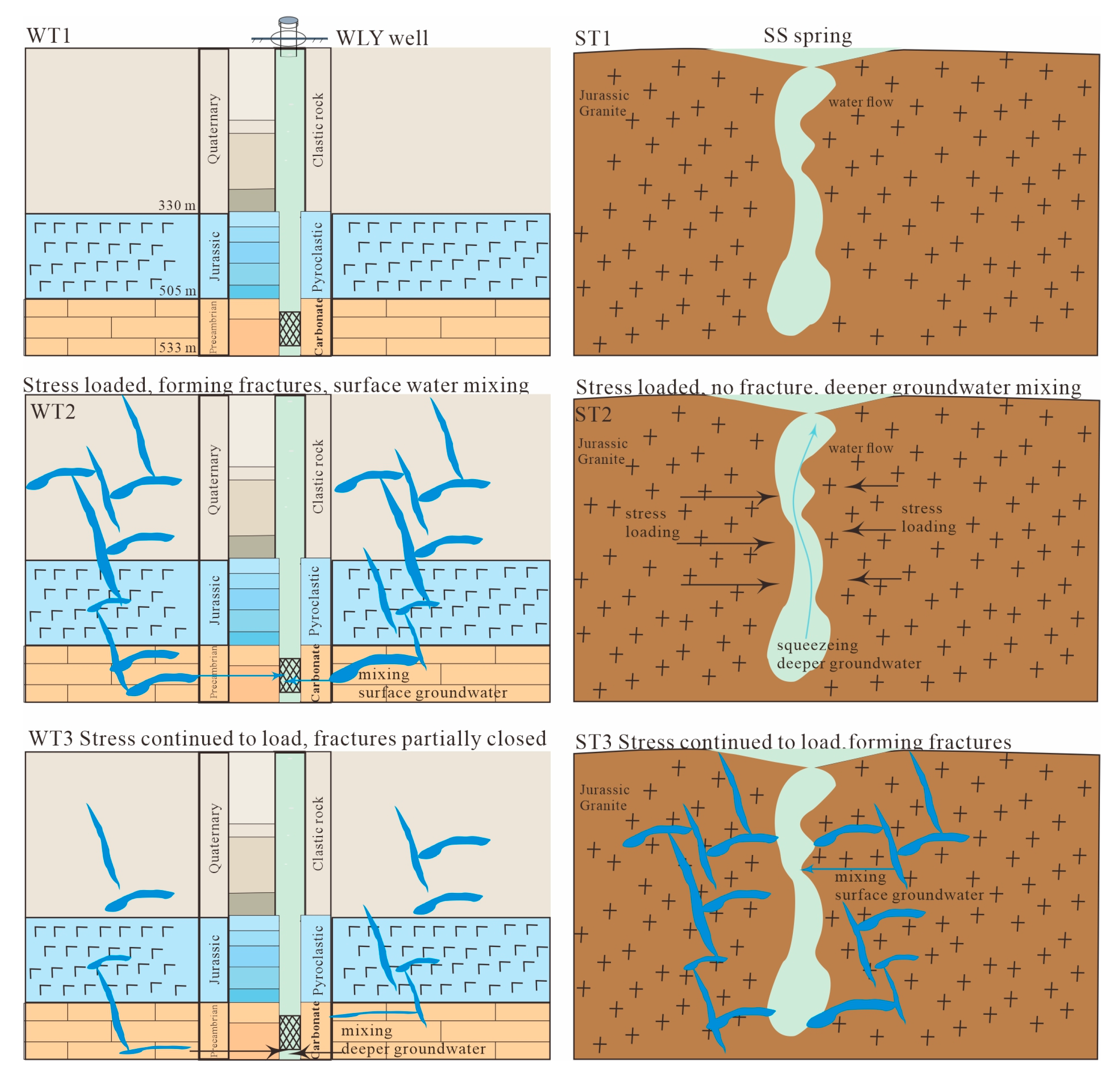
The differences in the time of rupture between carbonate and granite under sustained stress led to opposite patterns in isotopic changes. The carbonate rocks of the WLY aquifer were the first to form microfractures, mixing with surface water, resulting in peaks in isotopes values. The granites of the SS aquifer were not fractured, and deeper groundwater was squeezed into the column, resulting in lower isotope values.

(3)

δ²H and δ¹⁸O isotope variation is sensitive to changing stress states, highlight the potential importance of stable isotope indicators in earthquake-prediction studies.

References

1. De Luca, G.; Di Carlo, G.; Tallini, M. A record of changes in the Gran Sasso groundwater before, during and after the 2016 Amatrice earthquake, central Italy. Sci. Rep. 2018, 8, 15982. [Google Scholar] [CrossRef] [PubMed]
2. Huang, F.; Li, M.; Ma, Y.; Han, Y.; Tian, L.; Yan, W.; Li, X. Studies on earthquake precursors in China: A review for recent 50 years. Geod. Geodyn. 2017, 8, 1–12. [Google Scholar] [CrossRef]
3. Manga, M.; Wang, C.Y. Earthquake Hydrology, Treatise on Geophysics; Elsevier: Amsterdam, The Netherlands, 2015. [Google Scholar]
4. Martinelli, G. Previous, Current, and Future Trends in Research into Earthquake Precursors in Geofluids. Geosciences 2020, 10, 189. [Google Scholar] [CrossRef]
5. Montgomery, D.R.; Manga, M. Streamflow and water well responses to earthquakes. Science 2003, 300, 2047–2049. [Google Scholar] [CrossRef]
6. Roeloffs, E.A. Persistent water level changes in a well near Parkfield, California, due to local and distant earthquakes. J. Geophys. Res. 1998, 103, 869–889. [Google Scholar] [CrossRef]
7. Shi, Z.; Liao, F.; Wang, G.; Xu, Q.; Mu, W.; Sun, X. Hydrogeochemical Characteristics and Evolution of Hot Springs in Eastern Tibetan Plateau Geothermal Belt, Western China: Insight from Multivariate Statistical Analysis. Geofluids 2017. [Google Scholar] [CrossRef]
8. Toutain, J.; Munoz, M.; Poitrasson, F.; Lienard, A. Springwater chloride ion anomaly prior to a ML=5.2 Pyrenean earthquake. Earth Planet. Sci. Lett. 1997, 149, 113–119. [Google Scholar] [CrossRef]
9. Wang, C.Y.; Manga, M. Earthquakes and Water; Springer: Berlin/Heidelberg, Germany, 2010. [Google Scholar]
10. Yan, Y.; Zhang, Z.; Zhou, X.; Wang, G.; He, M.; Tian, J.; Dong, J.; Li, J.; Bai, Y.; Zeng, Z.; et al. Geochemical characteristics of hot springs in active fault zones within the northern Sichuan-Yunnan block: Geochemical evidence for tectonic activity. J. Hydrol. 2024, 635. [Google Scholar] [CrossRef]
11. Claesson, L.; Skelton, A.; Graham, C.; Dietl, C.; Mörth, M.; Torssander, P.; Kockum, I. Hydrogeochemical changes before and after a major earthquake. Geology 2004, 32, 641–644. [Google Scholar] [CrossRef]
12. Kopylova, G.N.; Boldina, S.V.; Serafimova, Y.K. Earthquake precursors in the ionic and gas composition of groundwater: A review of world data. Geochem. Int. 2022, 60, 928–946. [Google Scholar] [CrossRef]
13. Li, Y.; Chen, Z.; Hu, L.; Su, S.; Zheng, C.; Liu, Z.; Lu, C.; Zhao, Y.; Liu, J.; He, H. Advances in seismic fluid geochemis-try and its application in earthquake forecasing. Chin. Sci. Bull. 2022, 67, 1404–1420. [Google Scholar] [CrossRef]
14. Martinelli, G.; Dadomo, A. Factors constraining the geographic distribution of earthquake geochemical and fluid-related precursors. Chem. Geol. 2017, 469, 176–184. [Google Scholar] [CrossRef]
15. Poitrasson, F.; Dundas, S.H.; Toutain, J.-P.; Munoz, M.; Rigo, A. Earthquake-related elemental and isotopic lead anomaly in a springwater. Earth Planet. Sci. Lett. 1999, 169, 269–276. [Google Scholar] [CrossRef]
16. Shi, Z.; Zhang, H.; Wang, G. Groundwater trace elements change induced by M5.0 earthquake in Yunnan. J. Hydrol. 2020, 581. [Google Scholar] [CrossRef]
17. Thomas, D. Geochemical precursors to seismic activity. Pure Appl. Geophys. 1988, 126, 241–266. [Google Scholar] [CrossRef]
18. Wakita, H. Geochemical challenge to earthquake prediction. Proc. Natl. Acad. Sci. USA 1996, 93, 3781–3786. [Google Scholar] [CrossRef]
19. Skelton, A.; Liljedahl-Claesson, L.; Wästeby, N.; Andrén, M.; Stockmann, G.; Sturkell, E.; Mörth, C.; Stefansson, A.; Tollefsen, E.; Siegmund, H. Hydrochemical changes before and after earthquakes based on long-term measurements of multiple parameters at 2 sites in northern Iceland-A review. J. Geophys. Res. Solid Earth 2019, 124, 2702–2720. [Google Scholar] [CrossRef]
20. Skelton, A.; Andrén, M.; Kristmannsdóttir, H.; Stockmann, G.; Mörth, C.-M.; Sveinbjörnsdóttir, Á.; Jónsson, S.; Sturkell, E.; Guðrúnardóttir, H.R.; Hjartarson, H. Changes in groundwater chemistry before two consecutive earthquakes in Iceland. Nat. Geosci. 2014, 7, 752–756. [Google Scholar] [CrossRef]
21. Chen, Y.X.; Liu, J.B. Groundwater trace element changes were probably induced by the ML3.3 earthquake in Chaoyang district, Beijing. Front. Earth Sci. 2023, 11, 1260559. [Google Scholar] [CrossRef]
22. Chen, Y.X.; Liu, G.; Huang, F.; Wang, Z.; Hu, L.; Yang, M.; Sun, X.; Hua, P.; Zhu, S.; Zhang, Y. Multiple geochem-ical parameters of the Wuliying well of Beijing seismic monitoring networks probably responding to the small earthquake of Chaoyang, Beijing, in 2022. Front. Earth Sci. 2024, 12, 1448035. [Google Scholar] [CrossRef]
23. Hammer, O.; Harper, D.A.T. Paleontological Data Analysis; Blackwell Publishing: Oxford, UK, 2006; p. 351. [Google Scholar]
24. Harper, D.A.T. Numerical Palaeobiology: Computer-Based Modelling and Analysis of Fossils and Their Distributions; John Wiley & Sons: Hoboken, NJ, USA, 1999. [Google Scholar]
25. Copenhaver, M.D.; Holland, B. Computation of the distribution of the maximum studentized range statistic with application to multiple significance testing of simple effects. J. Stat. Comput. Simul. 1988, 30, 1–15. [Google Scholar] [CrossRef]
26. Kohonen, T. Self-organized formation of topologically correct feature maps. Biol. Cybern. 1982, 43, 59–69. [Google Scholar] [CrossRef]
27. Vesanto, J.; Himberg, J.; Alhoniemi, E.; Parhankangas, J. SOM Toolbox for Matlab 5; Espoo, Finland, 2000; Available online: http://www.cis.hut.fi/somtoolbox/package/papers/techrep.pdf (accessed on 20 April 2025).
28. Bai, Y.; Wang, G.; Shi, Z.; Zhou, X.; Yan, X.; Zhang, S.; Mao, H.; Wang, C. Hydrogeochemical changes with emphasis on trace elements in an artesian well before and after the September 8, 2018 Ms 5.9 Mojiang Earthquake in Yunnan, southwest China. Appl. Geochem. Appl. Geochem. 2024, 167. [Google Scholar] [CrossRef]
29. Ikotun, A.M.; Ezugwu, A.E.; Abualigah, L.; Abuhaija, B.; Heming, J. K-means clustering algorithms: A comprehensive review, variants analysis, and advances in the era of big data. Inf. Sci. 2023, 622, 178–210. [Google Scholar] [CrossRef]
30. Moore, J.W.; Semmens, B.X. Incorporating uncertainty and prior information into stable isotope mixing models. Ecol. Lett. 2008, 11, 470–480. [Google Scholar] [CrossRef]
31. Stock, B.C.; Jackson, A.L.; Ward, E.J.; Parnell, A.C.; Phillips, D.L.; Semmens, B.X. Analyzing mixing systems using a new generation of Bayesian tracer mixing models. PeerJ 2018, 6, 5096. [Google Scholar] [CrossRef]
32. Parnell, A.C.; Phillips, D.L.; Bearhop, S.; Semmens, B.X.; Ward, E.J.; Moore, J.W.; Jackson, A.L.; Grey, J.; Kelly, D.J.; Inger, R. Bayesian stable isotope mixing models. Environmetrics 2013, 24, 387–399. [Google Scholar] [CrossRef]
33. Craig, H. Isotopic variations in meteoric waters. Science 1961, 133, 1702–1703. [Google Scholar] [CrossRef]
34. Yu, J.S.; Yu, F.J.; Liu, D.P. The oxygen and hydrogen isotopic compositions of meteoric waters in the eastern part of China. Geochemistry 1987, 1, 22–26. (In Chinese) [Google Scholar] [CrossRef]
35. Li, J.; Shi, Z.; Wang, G.; Liu, F. Evaluating Spatiotemporal Variations of Groundwater Quality in Northeast Beijing by Self-Organizing Map. Water 2020, 12, 1382. [Google Scholar] [CrossRef]
36. Taylor, H.P. Water/rock interactions and the origin of H2O in granitic batholiths. J. Geol. Soc. 1977, 133, 509–558. [Google Scholar] [CrossRef]
37. Zhai, Y.Z.; Wang, J.S.; Teng, Y.G.; Zuo, R. Variations of δD and δ18O in Water in Beijing and Their Implications for the Local Water Cycle. Resour. Sci. 2011, 33, 92–97. (In Chinese) [Google Scholar]
38. Wei, X.; Yu, Y.L.; Li, W.Y.; Lu, C.C.; Huo, W.J. Hydrochemistry and isotopic characteristics of Guishui River Basin and their indicative significance. Environ. Sci. Technol. 2024, 47, 135–145. (In Chinese) [Google Scholar]
39. Scholz, C.H.; Sykes, L.R.; Aggarwal, Y.P. Earthquake prediction: A physical basis. Science 1973, 181, 803–810. [Google Scholar] [CrossRef]
40. Brace, W.F.; Paulding, B.W.; Scholz, C.J. Dilatancy in the fracture of crystalline rocks. J. Geophys. Res. 1966, 71, 3939–3953. [Google Scholar] [CrossRef]
41. Lockner, D.A.; Beeler, N.M. Rock Failure and Earthquakes. In International Handbook of Earthquake and Engineering Seismology; Part A; Lee, W.H.K., Kanamori, H., Jennings, P.C., Kisslinger, C., Eds.; Academic Press: Amsterdam, The Netherlands, 2002; pp. 505–537. [Google Scholar]
42. Gao, L. Study on Energy Evolution Mechanism and Catastrophe Characteristics During Rock Deformation and Failure; China University of Mining and Technology: Beijing, China, 2021. (In Chinese) [Google Scholar]
43. Lockner, D.A.; Byerlee, J.D.; Kuksenko, V.; Ponomarev, A.; Sidorin, A. Quasi-static fault growth and shear fracture energy in granite. Nature 1991, 35, 39–42. [Google Scholar] [CrossRef]
44. Zhao, Y.Z.; Qu, L.Z.; Wang, X.Z.; Cheng, Y.F.; Shen, H.C. Simulation experiment on prolongation law of hydraulic fracture for different lithologic formations. J. China Univ. Pet. (Ed. Nat. Sci.) 2007, 31, 63–66. (In Chinese) [Google Scholar]
45. Claesson, L.; Skelton, A.; Graham, C.; Mörth, C. The timescale and mechanisms of fault sealing and water-rock interaction after an earthquake. Geofluids 2007, 7, 427–440. [Google Scholar] [CrossRef]
46. Wästeby, N.; Skelton, A.; Tollefsen, E.; Andrén, M.; Stockmann, G.; Liljedahl, L.C.; Sturkell, E.; Mörth, M. Hydrochemical monitoring, petrological observation, and geochemical modeling of fault healing after an earthquake. J. Geophys. Res. Solid Earth 2014, 119, 5727–5740. [Google Scholar] [CrossRef]
47. Yang, N.; Wang, G.; Shi, Z.; Zhao, D.; Jiang, W.; Guo, L.; Liao, F.; Zhou, P. Application of Multiple Approaches to Investigate the Hydrochemistry Evolution of Groundwater in an Arid Region: Nomhon, Northwestern China. Water 2018, 10, 1667. [Google Scholar] [CrossRef]
48. Huang, F.Q.; Deng, Z.H.; Gu, J.P.; Wang, H.M.; Lu, P.L. Research of the field of subsurface fluid anomalies before the Zhangbei earthquake. Earthquake 2002, 22, 114–122. [Google Scholar]
49. Shi, Z.; Wang, G.; Liu, C. Advances in research on earthquake fluids hydrogeology in China: A review. Earthq. Sci. 2013, 26, 415–425. [Google Scholar] [CrossRef]
50. Zhou, Z.; Zhong, J.; Zhao, J.; Yan, R.; Tian, L.; Fu, H. Two Mechanisms of Earthquake-Induced Hydrochemical Variations in an Observation Well. Water 2021, 13, 2385. [Google Scholar] [CrossRef]
Figure 1. The earthquake distribution (A) in the Beijing area from June 2021 to June 2022. The biggest yellow circle is the Chaoyang ML3.3 earthquake. (B) The time sequence of earthquakes above ML1.6 (modified from Chen and Liu, 2023) [21]. The orange portions represent the statistical box plots of the magnitude of earthquakes in the year, and the error bars connect the smallest and largest data points. If only one earthquake occurred in a year, it is indicated by a red dot.
Geosciences 15 00192 g001
Figure 2. Four stages of time series variation of hydrogen and oxygen isotopes over sampling time at (A) WLY well and (B) SS spring. Purple vertical line shows time of biggest earthquake, Chaoyang ML3.3 earthquake. (C) Bivariant plots of δ2H-δ18O at WLY well (green circles) and SS spring (blue triangles). Global meteoric water line (GMWL) from [33] and local meteoric water line (LMWL) from [34] are shown. The green oval background indicates the three groups of WLY, and the green arrow lines indicate the development of WLY groups organized by time sequence. The blue oval background indicates the three groups of SS, and the blue arrow lines indicate the development of SS groups organized by time sequence.
Geosciences 15 00192 g002
Figure 3. The ANOVA tests for δ2H and δ18O across the four stages at WLY and SS. The results of the statistical tests form a table; Tukey’s Q is below the diagonal (the lower left triangle of the array) and probabilities p are above the diagonal (in the upper right). The nonsignificant values are orange. The black dots are isotopes data of WLY, the red triangle are isotopes data of SS. The red arrows indicate increased stages, the blue arrows indicate decreased stages. The values on the green background are close to 0.05, the values on the orange background are above 0.05.
Geosciences 15 00192 g003
Figure 4. Visualization of δ2H and δ18O from SOM and K-means clustering algorithm results for WLY well and SS spring. (A) Pattern of cluster formation for WLY well. (B) Pattern of cluster formation for SS spring.
Geosciences 15 00192 g004
Figure 5. Proportional contributions of three potential sources of groundwater. (A) Bivariant plots of δ2H-δ18O from three sources and all stages at WLY and SS. (B) Proportional contributions at WLY. (C) Proportional contributions at SS.
Geosciences 15 00192 g005
Figure 6. Concept model of three stages of δ2H and δ18O isotope change before earthquakes in WLY well and SS spring.
Geosciences 15 00192 g006
Disclaimer/Publisher’s Note: The statements, opinions and data contained in all publications are solely those of the individual author(s) and contributor(s) and not of MDPI and/or the editor(s). MDPI and/or the editor(s) disclaim responsibility for any injury to people or property resulting from any ideas, methods, instructions or products referred to in the content.