Abstract
Integrated facies and micropaleontological analyses of the late Piacenzian to early Gelasian, middle shelf to lower shoreface succession of the Strongoli area, southern Italy, reveal a hierarchy of transgressive–regressive sequences. In particular, higher rank sequences up to ca. 40 m thick, composed of transgressive systems tract, highstand systems tracts and falling stage plus lowstand systems tracts, are composed of 10–11 lower rank sequences 2.5–4 m thick. Some micropaleontological parameters were defined: distal/proximal (D/P; ratio between distal and proximal benthic foraminifera); fragmentation (Fr; percentage of fragmentation of benthic foraminifera); P/B (ratio between planktonic and benthic foraminifera); abundance (total count of individuals); diversity (sum of the recognized species). Among these parameters, the D/P and Fr are suitable, if used in conjunction, to recognize uncertainty intervals containing the maximum flooding surface (between the D/P maxima and Fr minima) and the maximum regressive surface (between D/P minima and Fr maxima). Moreover, combining these parameters with the sedimentological evidence, it is possible to recognize transgressive and regressive trends of different hierarchical ranks. The present results are an example illustrating how an integration of different types of data allows the recognition of high-frequency sequences in shelf settings associated with minor shoreline shifts, which would otherwise have been unrecognized on the basis of only one kind of data. The present integrated approach, therefore, provides a way to improve the resolution of sequence stratigraphic analyses.
1. Introduction
Stratigraphic sequences were typically described in shelf plus shoreface and deltaic successions and where transgressions and regressions are related with large facies and associated environmental changes, allowing a clear recognition of depositional trends and stratigraphic surfaces (e.g., [1,2,3] and references therein). In contrast, high-frequency sequences, consisting of sequences in the realm of fourth-order or lower rank stratigraphic frameworks (102–105 yrs [3,4,5]), in several cases are associated with limited shoreline and facies shifts and can be difficult to identify. Recent, detailed field studies of shoreface deposits have demonstrated that meter- to decameter-scale high-frequency sequences characterized by very modest facies changes can still be recognizable based on modern sequence stratigraphic principles [6,7,8,9], although the identification of usually cryptic sequence stratigraphic surfaces, in particular the maximum flooding surface (MFS), needs an integration with micropaleontological data, which at the same time highlight transgressive and regressive trends [10]. However, the recognition of high-frequency sequences associated with limited shoreline shift in fully shelf muddy deposits is a challenge, as the signal of lower rank transgressions and regressions, and the evidence of related surfaces, are progressively lost seaward, becoming unreadable in very distal settings. New research employing several kinds of data is therefore necessary to address this problem.
This study deals with the late Piacenzian to early Gelasian succession of the Crotone Basin, southern Italy. While previous similar studies in the study area focused on the identification of high-frequency sequences in shoreface deposits [7,9], this one deals primarily with relatively fine-grained shelf deposits, in order to define criteria for the recognition of meter- to decameter-scale high-frequency sequences on the basis of detailed field data and micropaleontological analyses. These results represent a further step to improve sequence stratigraphic principles, providing a new tool for high-resolution sequence stratigraphic analysis.
2. Geological Setting
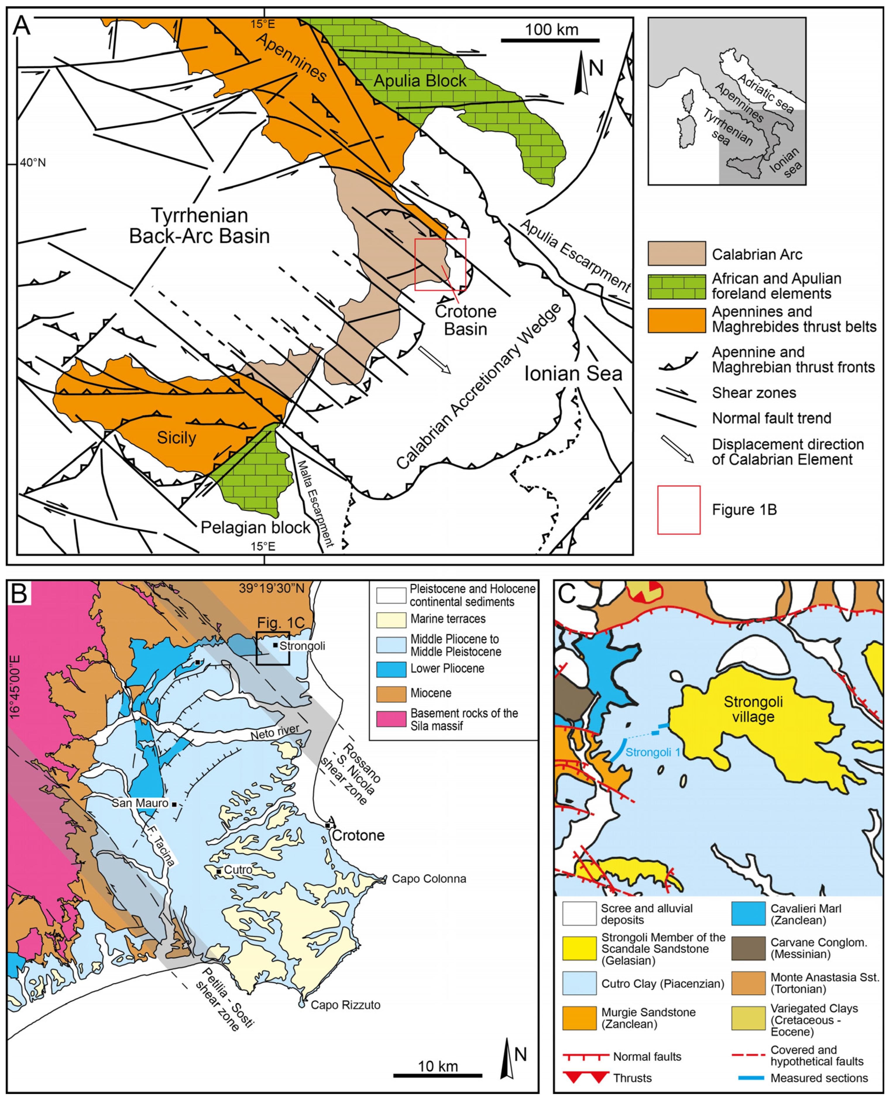
The Crotone Basin is a forearc depocenter developed since late Serravallian on the Ionian side of the Calabrian Arc (southern Italy), which consists of composite metamorphic, plutonic and sedimentary units and is located between the NW-trending southern Apennines and the E-trending Sicilian Maghrebides [11,12,13] (Figure 1A). The Calabrian Arc migrated to the SE since the Middle Miocene, and this process was accompanied by the subduction of the Ionian oceanic crust and the opening of the Tyrrhenian backarc basin [14,15,16,17,18,19,20,21,22] (Figure 1A).

Figure 1.
(A) Structural map of the Calabrian Arc and location of the Crotone Basin (modified from Van Dijk and Okkes [23]). (B) Simplified geologic map of the Crotone Basin, reporting the position of the study area shown in (C) (modified from Zecchin et al. [8,24]). (C) Geologic map of the study area in the northern part of the Crotone Basin, showing the position of the measured section (modified from Zecchin et al. [8]).
The Crotone Basin experienced alternating phases of tectonic subsidence and uplift plus basin closure [25,26,27,28,29,30,31,32], and its sedimentary succession consists of Serravallian to Middle Pleistocene marine, coastal and continental deposits, recording both tectonic events and glacio-eustasy [24,25,28,29,30,32] (Figure 1B and Figure 2). The middle Pleistocene part of the basin experienced tectonic uplift, which led to the emergence of its inner part and the formation of a staircase of marine terraces [33,34].
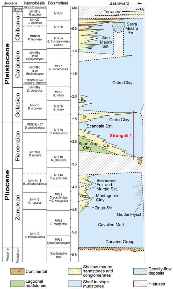
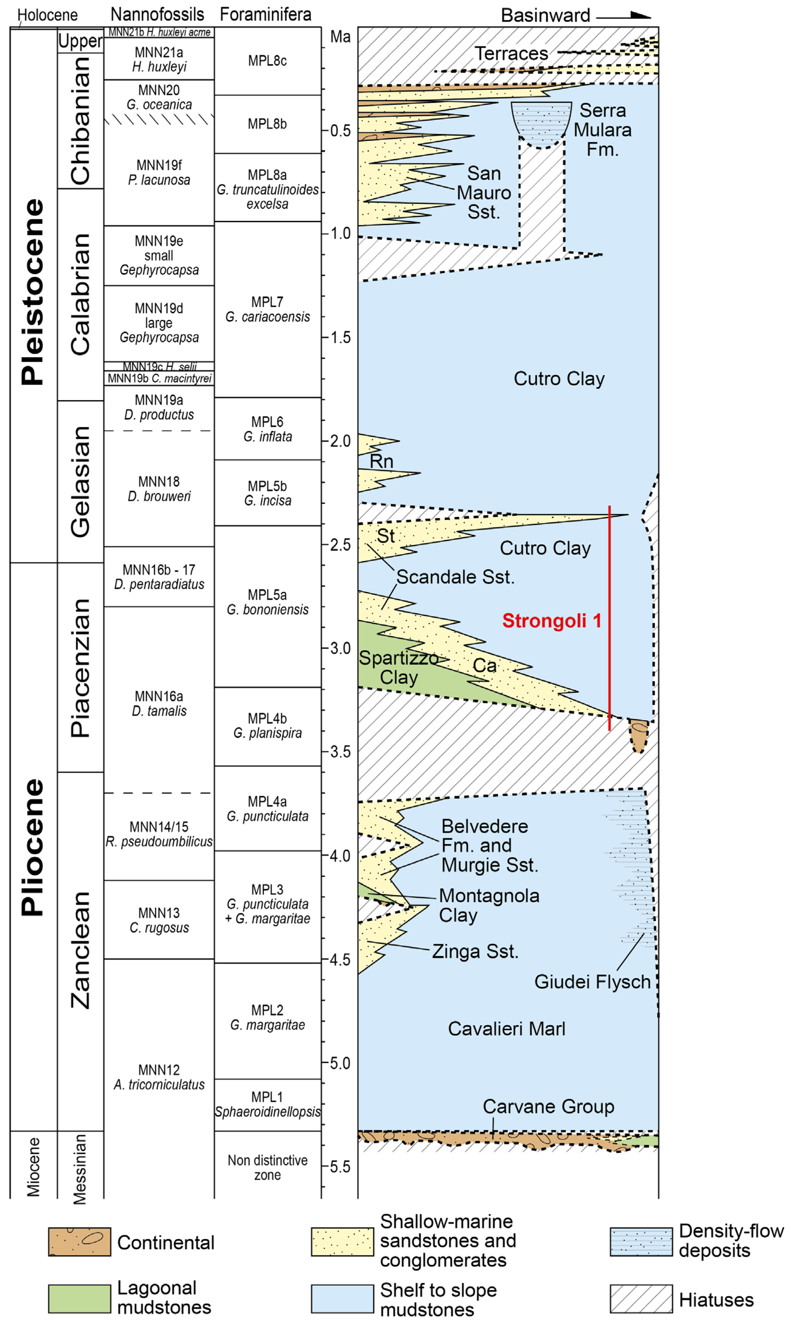
Figure 2.
The Plio-Pleistocene part of the sedimentary succession of the Crotone Basin (modified from Zecchin et al. [8,29]), compared with the IUGS International Chronostratigraphic Chart (https://stratigraphy.org/ICSchart/ChronostratChart2021-05.pdf (accessed on 12 March 2025)), and the calcareous nannofossil and planktonic foraminifera biostratigraphic schemes [35,36,37,38]. The studied succession (the Strongoli 1 section) comprises the lower part of the Piacenzian Cutro Clay and the Gelasian Strongoli Member of the Scandale Sandstone. Abbreviations: Ca: Casabona Member; Rn: Rocca di Neto Member; St: Strongoli Member.
3. Methods
A 67 m long measured section (Figure 3 and Figure 4) is the basis for this study, and a detailed facies analysis was performed for the recognition of facies and depositional environments (Table 1). Surfaces and depositional trends were recognized in order to define the sequence stratigraphic framework of the studied succession.


Figure 4.
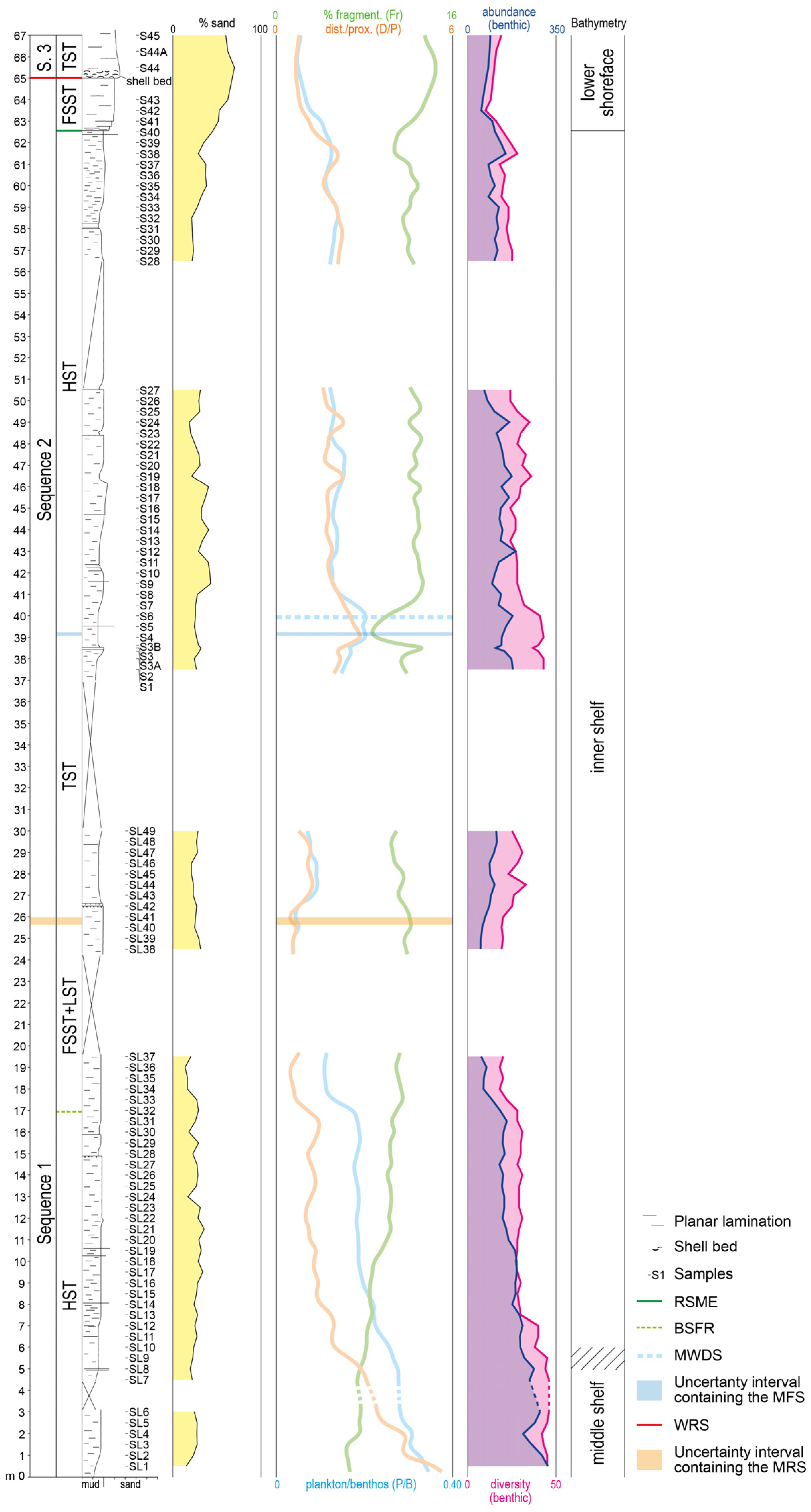
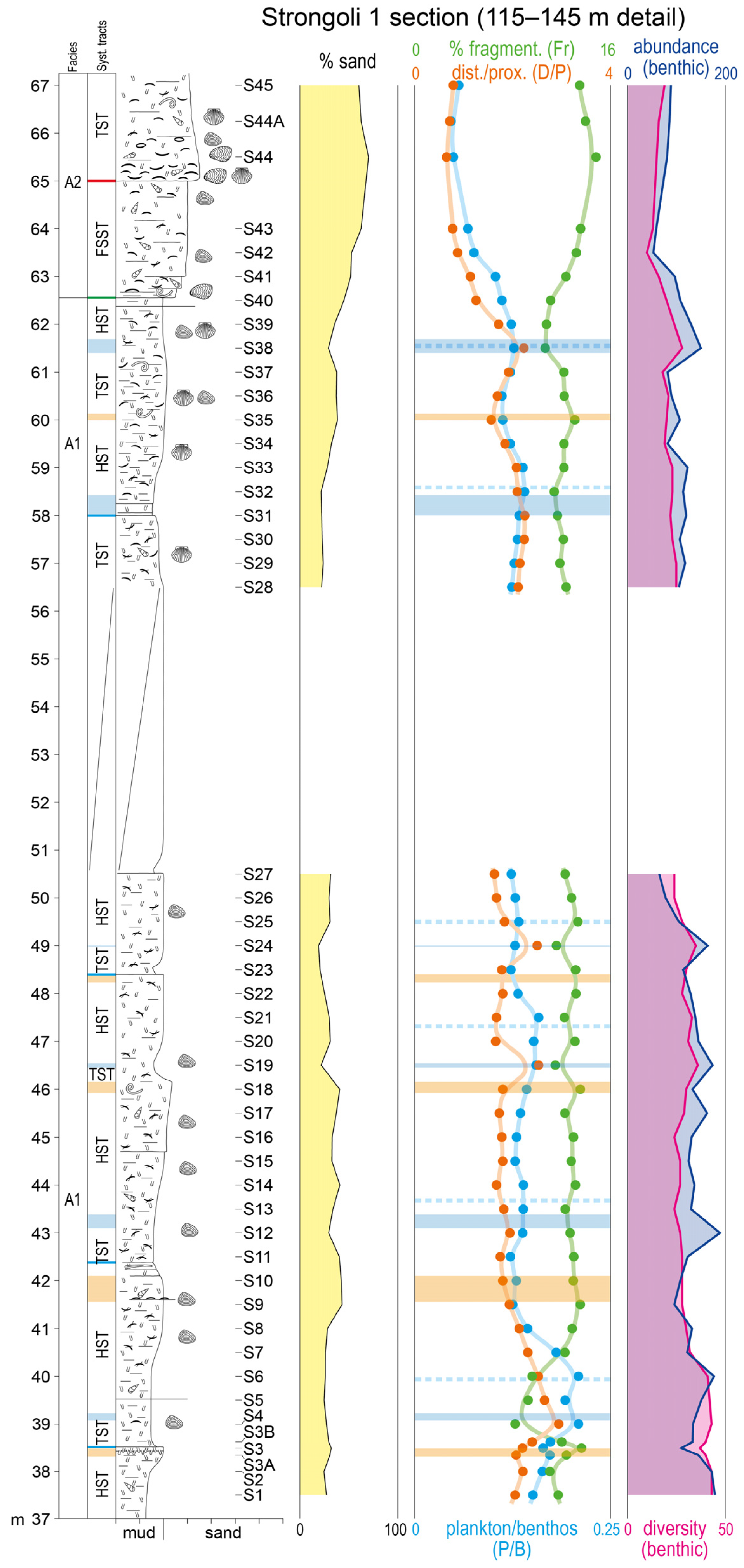
The measured section documenting part of the Cutro–Strongoli succession (see Figure 3). Lithology, percentage of sand, higher rank sequences (see text) and samples are shown on the left. Facies details are shown in Figure 5 and Figure 6. The curves derived from the micropaleontological analysis (abundance, diversity, Fr, D/P and P/B), and the inferred bathymetry, are shown on the right. Abbreviations: BSFR: basal surface of forced regression; FSST: falling-stage systems tract; HST: highstand systems tract; LST: lowstand systems tract; MFS: maximum flooding surface; MRS: maximum regressive surface; MWDS: maximum water depth surface; RSME: regressive surface of marine erosion; TST: transgressive systems tract; WRS: wave-ravinement surface.

Table 1.
Facies and depositional environments of the studied succession.
A total of 97 sediment samples were collected along the measured section (Figure 4), and approximately 100 g of sediment was taken from each sample for micropaleontological analyses. The sample aliquots were dried at 50 °C for 24 h and then treated with hydrogen peroxide (10% vol) for 12 h in order to remove the organic matter. Samples were then washed through a 125 μm mesh and dried. From the corresponding washing residues, 6 g of sediment was separated. All benthic foraminifera present in this amount of sediment were counted and classified following the taxonomic order of Loeblich and Tappan [42] and online catalogues on foraminifera, https://www.marinespecies.org/index.php (accessed on the 12 March 2025) and https://foraminifera.eu/ (accessed on the 12 March 2025)).
4. The Studied Succession
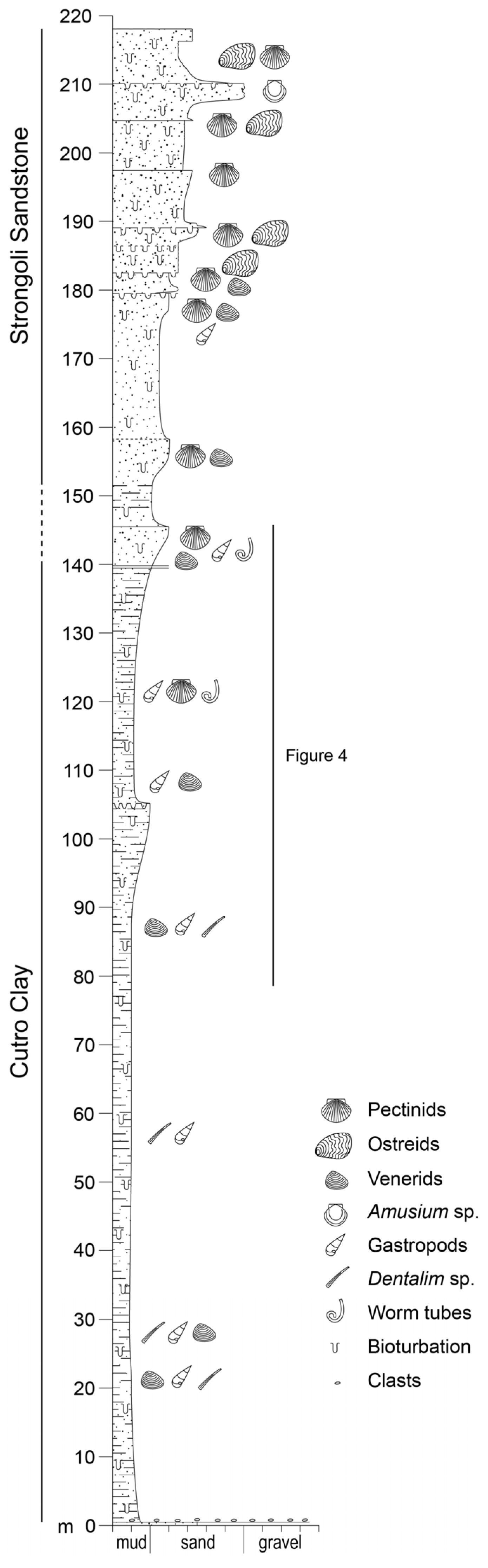
The studied deposits consist of part of the Piacenzian–Gelasian succession found in the northern part of the Crotone Basin, composed of the lower part of the Cutro Clay and the Strongoli Sandstone (also known as the Strongoli Member of the Scandale Sandstone [29]), which are, respectively, ca. 150 m and 70 m thick in the study area (Figure 1B,C, Figure 2 and Figure 3). These units were previously described by Roda [25], Capraro et al. [43] and Zecchin et al. [8,28,29], and they document a regressive trend from slope to shoreface settings (Figure 3). The studied interval of the Cutro Clay and Strongoli Sandstone succession is 67 m thick and starts at ca. 78 m from the base of the main section (Figure 3, Figure 4, Figure 5 and Figure 6). Facies and depositional environments of the studied interval are illustrated in Table 1.
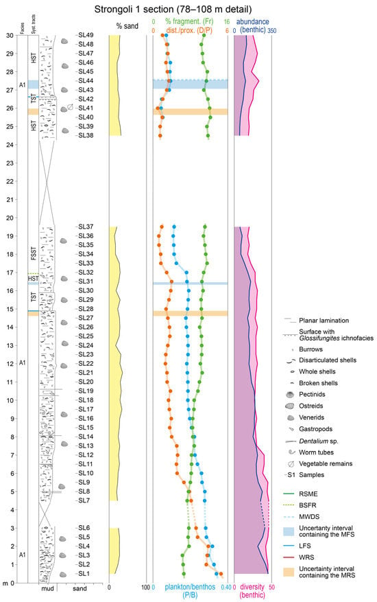
Figure 5.
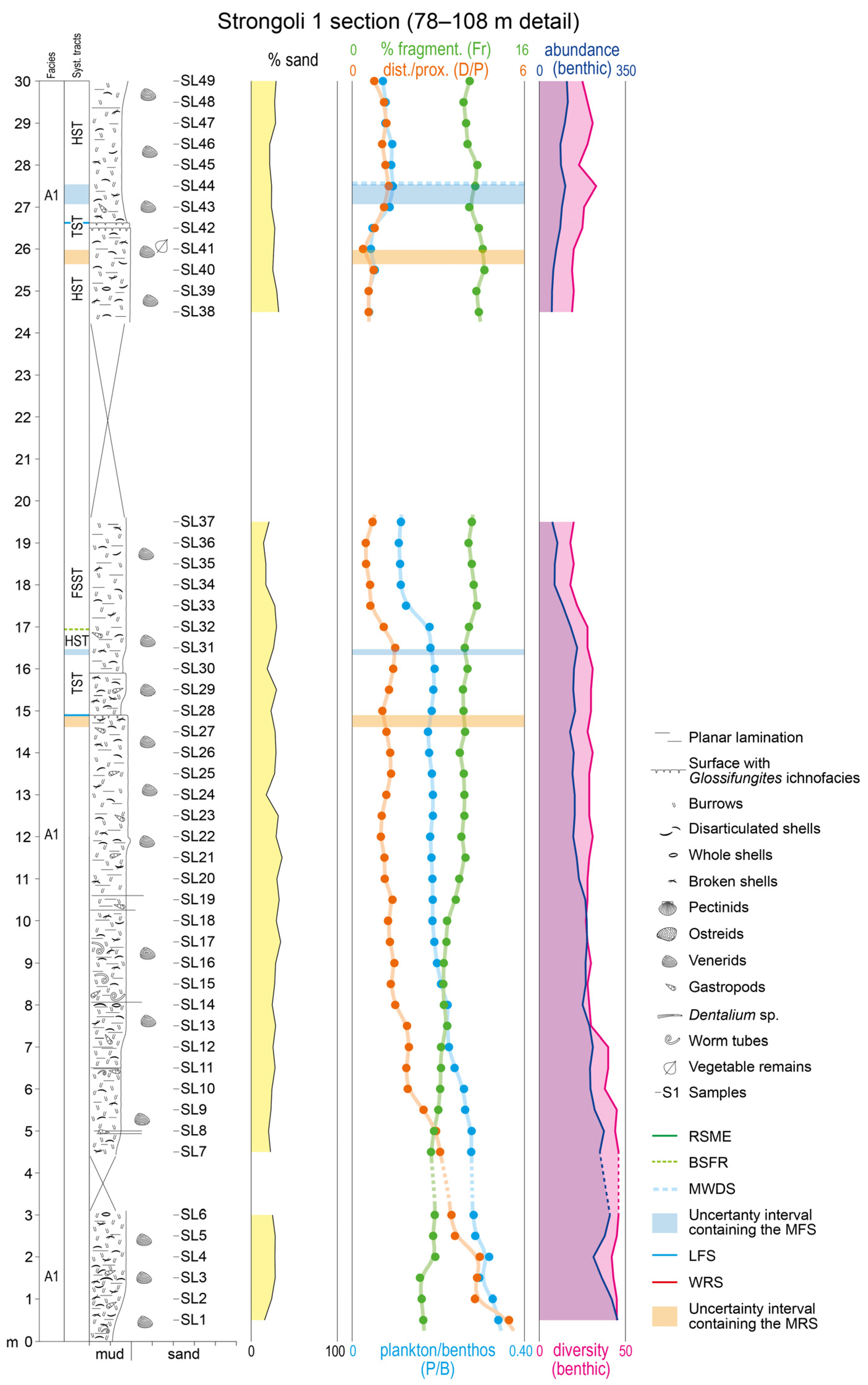
The lower part of the studied measured section (see Figure 4), reporting facies details (Table 1), lower rank systems tracts (see text), samples, percentage of sand and curves derived from the micropaleontological analysis (abundance, diversity, Fr, D/P and P/B). Abbreviations: BSFR: basal surface of forced regression; FSST: falling-stage systems tract; HST: highstand systems tract; LFS: local flooding surface; MFS: maximum flooding surface; MRS: maximum regressive surface; MWDS: maximum water depth surface; RSME: regressive surface of marine erosion; TST: transgressive systems tract; WRS: wave-ravinement surface.
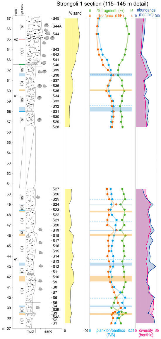
Figure 6.
The upper part of the studied measured section (see Figure 4), reporting facies details (Table 1), lower rank systems tracts (see text), samples, percentage of sand and curves derived from the micropaleontological analysis (abundance, diversity, Fr, D/P and P/B). See Figure 5 for symbols and abbreviations.
The Cutro Clay consists of clayey to sandy gray silt with occasional silty sand intervals, showing faint planar lamination and diffuse bioturbation (Facies A1; Table 1 and Figure 5, Figure 6 and Figure 7). It contains gastropods and bivalves that are usually small and thin, commonly disarticulated and fragmented but in places also whole, and worm tubes (Figure 5 and Figure 6). Minor grain size changes, underlined by well-defined surfaces locally marked by Glossifungites ichnofacies, are found (Figure 5, Figure 6 and Figure 8). These surfaces separate grain size cycles 2.5 to 4 m thick, ranging from clayey silt to sandy silt or even very fine-grained sand (Figure 5 and Figure 6). Finer grain sizes are usually found in the lower to middle part of these cycles.
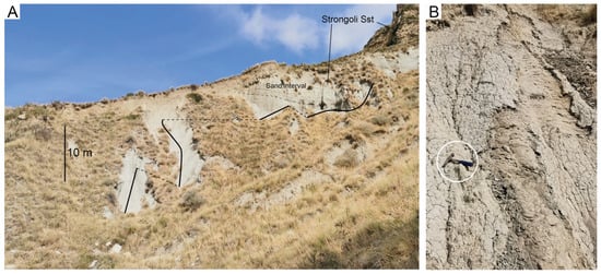
Figure 7.
(A) Field detail of the upper part of the measured section (black lines; see Figure 6) documenting part of the Cutro Clay and the sand interval representing the lowermost part of the Strongoli Sandstone (modified from Zecchin et al. [8]). (B) Detail of silt with faint planar lamination in the Cutro Clay.
The lowermost part of the Strongoli Sandstone, found in the upper part of the considered section (Figure 4 and Figure 6), consists of very fine- to fine-grained quartz sandstone, showing planar lamination, sparse bioturbation and larger mollusk shells (pectinids, ostreids, venerids and gastropods) with respect to the Cutro Clay (Facies A2; Table 1 and Figure 6 and Figure 9). The boundary between the Cutro Clay and the Strongoli Sandstone is sharp in the studied section (Figure 4, Figure 6 and Figure 9). The surface that separates the two units is planar and not associated with burrow traces, and the overlying sand coarsens upward from very fine- to fine-grained sandstone, up to another sharp, planar surface found in the middle of the measured sand interval (Figure 6 and Figure 9). This second sharp surface bounds the base of a 0.3 m thick shell bed composed of slightly coarser sand and containing disarticulated oysters, pectinids and minor gastropods (Figure 4 and Figure 6). An upward slightly decreasing grain size trend is found starting from the top of this shell bed (Figure 6). Overall, the studied succession documents a transition from middle to inner shelf (Cutro Clay) and lower shoreface settings (Strongoli Sandstone) (Table 1).
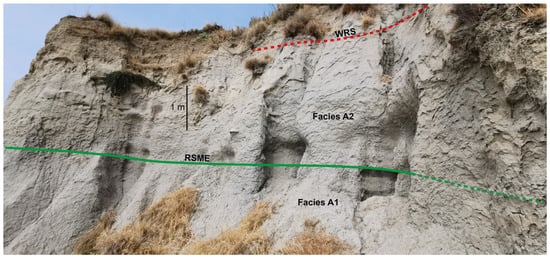
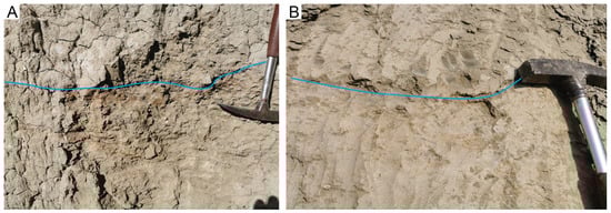
Figure 9.
Regressive surface of marine erosion (RSME) separating shelf siltstones (below) from very fine- to fine-grained, forced regressive sandstones in the upper part of the measured section (see Figure 6). A wave-ravinement surface (WRS) bounding the base of transgressive sandstones is found above. See Table 1 for facies characteristics.
5. Micropaleontological Analysis
5.1. Distribution of Benthic and Planktonic Foraminifera
The analysis of benthic micro-foraminifera has allowed us to recognize an overall shallowing-upward trend in the studied succession (Figure 4). According to studies by various authors [44,45,46,47,48,49,50,51,52] on the ecological behavior and across shelf distribution of benthic foraminifera, the following relatively distal species were identified: Uvigerina spp., Bolivina spp., Bulimina spp., Lenticulina spp., Amphycorina scalaris, Bigenerina nodosaria, Cibicidoides pseudoungerianus, Globobulimina affinis, Planulina ariminensis, Nonion fabum (Supplementary Materials). The relatively proximal species consist of Ammonia parkinsoniana, Ammonia tepida, Ammonia beccarii, Elphidium spp., Lobatula lobatula and Textularia spp. ([44,45,46,48,49,50,51,52,53]) (Supplementary Materials). The abundance of relatively distal species overall decreases upward, whereas the opposite occurs for relatively proximal species, reflecting an upward transition from middle to inner shelf depositional settings, and then to lower shoreface settings [44,45,46,47,48,49,50,51,52,53]. This evidence matches the results achieved from facies analysis (Table 1).
As for the planktonic foraminifera, the most common species are Globigerina bulloides, Globigerina ruber, Globorotalia inflata and Orbulina universa. In accordance with the indications provided by the benthic foraminifera, the abundance of planktonic foraminifera overall decreases upwards (see Supplementary Materials).
5.2. Parameters for Sequence Stratigraphy
Following Zecchin et al. [7,8,9,10], some micropaleontological parameters were calculated to recognize, in combination with the sedimentological evidence, transgressive–regressive trends and bathymetric changes. In particular, the ‘abundance’ (total count of individuals) and ‘diversity’ (sum of the recognized species) of benthic foraminifera (Figure 4, Figure 5 and Figure 6) were already used to recognize bathymetric trends and maximum flooding conditions in stratigraphic sequences [54,55]. However, the parameters introduced by Zecchin et al. [7,8,10], such as the ‘% fragmentation’ (Fr; the percentage of fragmentation of intra-basinal benthic foraminifera for each sample) and the ‘distal/proximal’ (D/P; the ratio between relatively distal and proximal species of benthic foraminifera for each sample), together with the well-known ‘plankton/benthos’ ratio (P/B; the ratio between the number of planktonic foraminifera and benthic foraminifera for each sample) (Figure 4, Figure 5 and Figure 6), have demonstrated greater accuracy in identifying the maximum flooding surface (MFS) and the point reflecting maximum water depth. In particular, the Fr parameter is calculated as follows:
Fr = (number of fragmented specimens/total number of specimens) × 100
According to Zecchin et al. [7,8,9,10], the Fr parameter reflects the environmental energy, which in turn can vary due to local energy changes and/or shoreline shifts, whereas the D/P parameter is thought to reflect variations of sedimentation rates linked to shoreline shifts and therefore is expected to be associated with transgressive and regressive trends. Zecchin et al. [7,8,9,10] demonstrated with a good degree of confidence that maximum values of the D/P parameter, concomitant with minimum values of the Fr parameter, reflect maximum flooding conditions. In particular, the relatively small interval between the positive peak of the D/P parameter and the negative peak of the Fr parameter, within a given stratigraphic sequence, defines an uncertainty interval within which the MFS should lie (Figure 4, Figure 5 and Figure 6). Unlike the D/P parameter, the P/B parameter is thought to be sensitive to water depth changes, and therefore its positive peak within a stratigraphic sequence, in general not coinciding with the positive peak of the D/P parameter (Figure 4, Figure 5 and Figure 6), reflects maximum water depth conditions (i.e., the maximum water depth surface ‘MWDS’ [7,8,9,10]).
As highlighted by Zecchin et al. [10], the distal and proximal species of benthic foraminifera used to calculate the D/P parameter can vary depending on the considered distal-proximal transect. In the present case, the relatively proximal species of benthic foraminifera vary along the measured section. In particular, from 0 to 30 m (Figure 5), Ammonia beccarii, Lobatula lobatula and Textularia spp. are significant among the relatively proximal species, showing an overall upward increase in their abundance, whereas this is not true for the upper part of the section (from 37 m up, Figure 6), where these species are not considered and are replaced by more proximal ones.
Therefore, for the lower part of the section, the D/P parameter is calculated as follows:
D/P = (%Uvigerina spp. + %Bolivina spp. + %Bulimina spp. + Lenticulina spp. + %Amphycorina scalaris + %Bigenerina nodosaria + %Cibicidoides pseudoungerianus + %Globobulimina affinis + %Planulina ariminensis + %Nonion fabum)/(%Ammonia parkinsoniana + %Ammonia tepida + %Ammonia beccarii + %Elphidium spp. + %Lobatula lobatula + %Textularia spp.)
For the upper part of the section, the D/P parameter is calculated in the same way but without the % of Ammonia beccarii, Lobatula lobatula and Textularia spp.
The distribution of the considered distal and proximal species may also depend on environmental factors, such as the concentration of organic matter [56]. However, the good match between the D/P and Fr curves suggests a prevailing control by shoreline shifts.
Overall, the D/P, P/B, ‘abundance’ and ‘diversity’ curves vary in a similar way, with higher values in the lower part of the measured section and some positive and negative peaks that are clearer following the D/P and P/B parameters (Figure 4, Figure 5 and Figure 6). The Fr curve, instead, exhibits an opposite trend, and in the middle to upper part of the section it is almost specular with respect to the D/P curve (Figure 4, Figure 5 and Figure 6). While usually the positive peaks of the P/B curve slightly follow those of the D/P curve, the positive ones of the ‘abundance’ and ‘diversity’ curves in some cases are close to those of the D/P and in others to those of the P/B (Figure 4, Figure 5 and Figure 6). The significance of these variations is explained in the next section.
6. Sequence Stratigraphy
6.1. Higher Rank Sequences
Following the curves relative to the calculated micropaleontological parameters, an overall upward decrease in the D/P, P/B, ‘abundance’ and ‘diversity’ parameters is recognizable in the lower part of the measured section, up to an interval of minimum values between ca. 18 and 26 m from the base (Figure 4). In contrast, the Fr parameter shows a parallel increase up to a relative maximum at ca. 26 m from the base of the section (Figure 4). The D/P, P/B, ‘abundance’ and ‘diversity’ parameters then show an overall increase up to a relative maximum between 39 and 40 m from the base, whereas the Fr parameter shows the opposite (Figure 4). Excepting for the higher values at the base of the section, this positive peak of the D/P and the other parameters is the highest of the section (excepting for the ‘abundance’), whereas the negative peak of the Fr parameter is the lowest (Figure 4). Finally, the D/P, P/B, ‘abundance’ and ‘diversity’ parameters show an overall slight, irregular decrease up to another relative minimum above 63 m from the base of the section, within the sandy unit, whereas relatively high values are shown by the Fr parameter in this sandy unit (Figure 4). The % of sand shows an overall slight increase in the lower to middle part of the section and a more marked increase above 61.5 m from the base (Figure 4).
These variations suggest the presence of a cyclicity within the measured section. In particular, following Section 5, the combined variations of the D/P and Fr parameters indicate the presence of alternating regressive (from the base to ca. 26 m, and from ca. 39 and 65 m) and transgressive (from ca. 26 and 39 m, and above 65 m) trends (Figure 4). In particular, the overall decrease in the D/P parameter and the increase in the Fr parameter in the lower part of the section could reflect normal regressive progradation, as also testified by the gradual decrease in the P/B parameter, which is inferred to reflect the bathymetric trend (Section 5). This gradual decrease is also testified by the ‘abundance’ and ‘diversity’ parameters (Figure 4).
An abrupt bathymetric lowering is highlighted by a rapid decrease in the P/B parameter at ca. 17 m from the base (Figure 4), and this is also accompanied by a similarly marked decrease in the D/P, ‘abundance’ and ‘diversity’ parameters, and by an increase in the Fr parameter, suggesting an overall acceleration in the regressive trend probably accompanied by relative sea level fall. Such evidence suggests that the gradual regressive trend found between the base of the section and ca. 17 m reflects highstand progradation (highstand systems tract, HST), followed by forced regression (falling-stage systems tract, FSST) (Figure 4). A basal surface of forced regression (BSFR) [57] is therefore inferred to be placed at ca. 17 m, at the beginning of the abrupt bathymetric decrease (Figure 4).
Similarly to Zecchin et al. [7,8,9,10], who defined an uncertainty interval containing the MFS between a relative maximum of the D/P curve and a relative minimum of the Fr curve, another uncertainty interval is introduced here between a relative minimum of the D/P curve and a relative maximum of the Fr curve, which should contain the maximum regressive surface (MRS) [58], in this case just below 26 m from the base of the section and ca. 0.3 m thick (Figure 4). It should be noted that the resolution provided by the ‘abundance’ and ‘diversity’ curves does not allow such a thin interval to be defined but only a relatively large interval of minimum values between ca. 18 and 26 m from the base (Figure 4).
The inferred MRS falls in an interval of the section that does not have any physical expression in the field, although it is slightly coarser grained than the lower part of the section and that immediately above (Figure 4). The uncertainty interval containing the MRS seems to be followed by a slight decreasing trend of the % of sand, as expected [2,3] (Figure 4). The interval comprised between the inferred BSFR and the MRS is ca. 9 m thick and should correspond to a shelf FSST and possibly to part of the lowstand systems tract (LST) (Figure 4). The eventual correlative conformity (CC) [59] could be placed in the cover interval between 19.5 and 24.5 m.
The marked positive peak of the D/P parameter and the negative peak of the Fr parameter at ca. 39 m from the base of the section define the uncertainty interval, ca. 0.15 m thick, containing the MFS (Figure 4). This implies that the interval of the section between the inferred MRS and MFS is a transgressive systems tract (TST) ca. 13 m thick, characterized by coastal retrogradation and bathymetric increase, as highlighted by the increase of the D/P and P/B parameters and by an overall decrease in the Fr parameter (Figure 4). Also, the ‘abundance’ and ‘diversity’ curves document an overall increase (Figure 4). The TST is characterized by an overall decrease in grain size, and its lowermost part is marked by surfaces characterized by substrate-controlled ichnofacies (Figure 4 and Figure 8B), reflecting sediment starvation in the shelf during coastal retreat [60].
The uncertainty interval containing the MFS is followed by the second HST of the studied succession, ca. 23.5 m thick, which is characterized by slight decreases in the D/P, P/B, ‘abundance’ and ‘diversity’ curves and a relatively constant Fr curve with minor changes, between 41 and 62.5 m from the base (Figure 4). This HST is featured by meter-scale changes in grain size reflecting a lower rank cyclicity (see Section 6.2) and an overall increase in the sand content in its upper part (Figure 4). Conditions of maximum water depth are thought to coincide with the positive peak of the P/B curve, corresponding to the MWDS (Section 5) (Figure 4). As expected, the MWDS does not coincide with the MFS and is placed slightly above, in the lowermost part of the HST [7,8,9,10] (Figure 4).
The sharp-based sandy unit of the succession, above ca. 62.5 m from the base and characterized by lower values of the D/P, P/B, ‘abundance’ and ‘diversity’ curves and higher values of the Fr curve (Figure 4), reflects a marked seaward shoreline shift and bathymetric decrease, probably due to forced regressive conditions after the accumulation of the HST. Following the specular D/P and Fr curves, maximum regressive conditions fall approximately at the surface bounding the base of a shell bed at ca. 65 m from the base (Figure 4), which is followed by renewed increases in the D/P, P/B, ‘abundance’ and ‘diversity’ curves and a decrease in the Fr curve as well as in the grain size. Based on this evidence, the erosional surface at ca. 62.5 m, separating the inner shelf and lower shoreface deposits, is interpreted as a regressive surface of marine erosion (RSME) [61,62], which reworked the BSFR and therefore bounds the base of a thin FSST only ca. 2.5 m thick (Figure 4 and Figure 9). The surface at ca. 65 m, at the base of the shell bed, is interpreted as a wave-ravinement surface (WRS) [63,64,65,66], reworking the MRS and bounding the base of the next TST (Figure 4). The shell bed can be interpreted as an onlap shell bed (OSB), produced by sediment bypass during transgression just above the WRS [67,68]. LST deposits, between the FSST and the TST, are inferred to have been accumulated seaward.
The present interpretation of the available data, therefore, allows us to recognize two higher rank sequences (Sequences 1 and 2, Figure 4), here arbitrarily separated by the MRS at ca. 26 m from the base of the section and the lowermost part of a third sequence above 65 m, bounded by the WRS plus MRS (Figure 4). Sequence 1 is incomplete and is represented by only the HST and the FSST plus LST (Figure 4). The thickness of its measured part is ca. 26 m. Sequence 2, ca. 39 m thick, is complete and consists of the TST, the HST and the FSST (Figure 4). The considered part of Sequence 3 is composed of only the lowermost TST (Figure 4).
The fact that the facies of Sequence 1 are on average more distal than those of Sequence 2, as evident by comparing the FSSTs, reflects the overall shallowing-upward trend of the whole succession (Figure 3). The lack of other correlatable sections prevents documentation of the lateral variability and the 3D architecture of the recognized sequences.
6.2. Lower Rank Sequences
As stated in Section 4, grain size cycles 2.5 to 4 m thick, ranging from clayey silt to sandy silt or even very fine-grained sand, are found in the studied succession, excepting for the lower 15 m of the measured section (Figure 5 and Figure 6). These cycles contain, or are separated by, sharp, flat surfaces associated with abrupt grain size decreases and locally with Glossifungites ichnofacies (Figure 5, Figure 6 and Figure 8A). The cycles are usually accompanied by coherent variations of the % of sand and in particular by marked higher frequency changes in the considered micropaleontological parameters (Figure 5 and Figure 6).
The recognition of the lower cycle, from ca. 15 and 19.5 m (Figure 5), is uncertain, as the signal provided by the micropaleontological data is not clear for all parameters. A relative minimum of the D/P curve and a maximum of the Fr curve allow us to define an uncertainty interval ca. 0.3 m thick just below 15 m, inferred to contain a high-frequency MRS (Figure 5). This interval is bounded at the top by a sharp surface marked by Glossifungites ichnofacies (Figure 5). In contrast, a relative maximum of the D/P curve and a minimum of the Fr curve allow us to recognize an uncertainty interval ca. 0.1 m thick at ca. 16.4 m from the base of the section, inferred to contain a high-frequency MFS (Figure 5). The other curves do not indicate such a cycle, and no curves provide significant evidence of a cyclicity below 15 m from the base of the section (Figure 5).
Since the inferred cycle from ca. 15 and 19.5 m is highlighted by the D/P and Fr parameters and by the presence of substrate-controlled ichnofacies, it is inferred to reflect minor shoreline shifts and associated transgressive–regressive trends. The cycle is therefore considered a high-frequency sequence composed of a TST between the MRS and the MFS and an HST just above the MFS (Figure 5). The surface marked by Glossifungites ichnofacies at ca. 15 m is interpreted as a local flooding surface (LFS) produced by sediment starvation in the shelf during transgression [60] (Figure 5). The marked lowering of the D/P, P/B, ‘abundance’ and ‘diversity’ curves found for the higher rank sequences at ca. 17 m (Section 6.1), and inferred to correspond to a BSFR (Figure 4), is interpreted in the same way for the lower rank sequence found between ca. 15 and 19.5 m, and therefore such a BSFR is thought to also separate a lower rank HST from a lower rank FSST (Figure 5).
The cover interval between 19.5 and 24.5 m prevents documentation of the top of the first high-frequency sequence and the lower part of the next one (Figure 5). Another relative minimum of the D/P curve and a maximum of the Fr curve just below 26 m allow us to recognize an uncertainty interval containing an MRS (Figure 5), which coincides with the MRS separating the higher rank Sequences 1 and 2 (Section 6.1; Figure 4). The presence of a relative maximum of the D/P curve and a minimum of the Fr curve above 27 m allows for documentation of another uncertainty interval, ca. 0.4 m thick, containing a high-frequency MFS and therefore a second high-frequency sequence between ca. 26 and 30 m (Figure 5). In this case, the positive peak of the D/P curve is accompanied also by similar peaks of the P/B, ‘abundance’ and ‘diversity’ curves (Figure 5), suggesting more marked maximum flooding conditions with respect to the lower high-frequency sequence. The positive peak of the P/B curve is slightly above the uncertainty interval, indicating conditions of maximum deepening at ca. 27.5 m (Figure 5). This sequence is inferred to be composed of a TST ca. 1.5 m thick, containing surfaces marked by Glossifungites ichnofacies and interpreted as an LFS, and by an HST (Figure 5). The top of the sequence is masked by the cover interval between 30 and 37 m. There are no clear elements to establish if the thin interval comprised between 24.5 m and the MRS just below 26 m is either a lower rank HST or FSST of the lower sequence, and in the absence of marked changes in the D/P, P/B and Fr curves, that interval has been tentatively assigned to the former (Figure 5).
Above the cover interval between 30 and 37 m from the base of the section, grain size variations and trends in the micropaleontological parameters are in general coherent and well readable. Six uncertainty intervals 0.05 to 0.3 m thick, between positive peaks of the D/P curve and negative peaks of the Fr curve, are well recognizable between 37 and 62.5 m, and they are interpreted to contain high-frequency MFSs (Figure 6). In general, but not in all cases, the positive peaks of the D/P curve are accompanied by higher values also for the P/B, ‘abundance’ and ‘diversity’ curves (Figure 6). The uncertainty interval at ca. 39 m is associated with the more marked positive peak of the D/P parameter and negative peak of the Fr parameter (Figure 6), and it coincides with the one containing the MFS of the higher rank Sequence 2 (Section 6.1; Figure 4). In almost all cases, the relative maximum of the P/B curve follows that of the D/P curve, indicating that maximum water depth conditions (corresponding to the MWDS) follow maximum flooding conditions, as expected [7,8,9,10] (Figure 6).
As for the uncertainty intervals containing the MRS, in the 37–62.5 m interval of the succession, they are not always defined between relative minima and maxima of the D/P and Fr curves, respectively, as in this case, the intervals so defined would have been very large and would not have had a perfect correspondence with the observed grain size variations and physical structures. Only the uncertainty intervals at ca. 38.5 and 60 m are defined between a negative peak in the D/P curve and a positive peak in the Fr curve, whereas the others are defined between a relative maximum of the Fr curve and the next sharp surface interpreted as an LFS, or the next grain size maximum (Figure 6).
With the uncertainty intervals containing the MFS and the MRS so defined, the interval of the succession between 37 and 62.5 m appears to be composed of high-frequency sequences 2.5 to 4 m thick, each of which is made up of a TST and an HST (Figure 6). Moreover, the sequences between 38.5 and 50.5 m show an architecture similar to that of a parasequence, with a relatively thin TST and a thicker HST, whereas those between 56.5 and 62.5 m show system tracts of a similar thickness (Figure 6). In general, HSTs exhibit a gradual grain size increase, whereas TSTs show smaller grain sizes (Figure 6). LFSs, where present, can be placed at the base, at the top, or within TSTs (Figure 6).
The upper part of the succession between 62.5 and 67 m, containing the FSST of the higher rank Sequence 2 and the TST of Sequence 3 (Section 6.1; Figure 4 and Figure 9), cannot be further subdivided, and such system tracts are considered also for the lower rank sequences (Figure 6).
Taking into account the covered intervals of the succession, Sequence 2, which is the complete one, is inferred to contain 10 or 11 lower rank sequences.
7. Discussion
The integration of sedimentological and micropaleontological data have allowed us to recognize two orders of cyclicity in the studied Piacenzian to Gelasian succession. In these mainly shelf deposits, grain size changes and substrate-controlled ichnofacies allow the recognition of a lower rank cyclicity in the middle to upper part of the succession, as well as the presence of sharp-based shoreface deposits in the upper part of the succession (Figure 5 and Figure 6). However, only the integration of the sedimentological evidence with the considered micropaleontological parameters, and in particular the D/P and Fr (Section 5), provides a clearer documentation of both lower and higher rank cyclicities (Figure 4, Figure 5 and Figure 6).
Since both higher and lower rank cyclicities are featured by coherent variations in the D/P and Fr parameters, which systematically exhibit contraposed minima and maxima, the recognized cyclicity is inferred to be associated with shoreline shifts and alternating transgressive–regressive trends [8,10]. These cycles can therefore be classified as stratigraphic sequences of different rank and separated by MRSs [4,69], in which ca. 10–11 lower rank sequences up to ca. 4 m thick compose up to ca. 40 m thick higher rank sequences (Figure 4, Figure 5 and Figure 6). The recognition of uncertainty intervals containing MRSs between the relative minima of the D/P parameter and maxima of the Fr parameter, and uncertainty intervals containing MFSs between the relative maxima of the D/P parameter and minima of the Fr parameter (Figure 4, Figure 5 and Figure 6), is a key element to subdivide the studied succession in stratigraphic sequences. Overall, the ‘abundance’ and ‘diversity’ parameters reflect the variations in the D/P parameter but with less precision, and in some cases, their peaks are close to those of the P/B parameter (Figure 4, Figure 5 and Figure 6). Both lower and higher rank uncertainty intervals containing the MFS tend to be followed by a relative maximum of the P/B curve, which reflects maximum water depth conditions (the MWDS) within stratigraphic sequences just in the lower part of the HST (Figure 4, Figure 5 and Figure 6), as expected in shelf successions experiencing a delayed basin shallowing due to sediment accumulation [7,8,9,10].
The evidence that higher rank sequences are composed of a TST, an HST and an FSST (plus LST), the latter being associated with an abrupt bathymetric decrease and an RSME at the base of forced regressive shorefaces (Figure 4 and Figure 9), highlights that such sequences are controlled by relative sea level changes, leading to shoreline shifts and parallel seaward and landward translations of facies tracts. The evidence that, excepting for the intervals of the succession corresponding to the FSSTs of the higher rank sequences, the lower rank ones seem to be composed of only TSTs and HSTs (Figure 5 and Figure 6), indicates that minor relative sea level falls were absent and that shoreline shifts were associated with only sediment supply changes and/or changes in the rate of relative sea level rise. Such minor shoreline shifts and associated translations of facies tracts justify the progressive loss of evidence of the lower rank cyclicity toward distal depositional settings, that is, toward to the lower part of the succession (Figure 5).
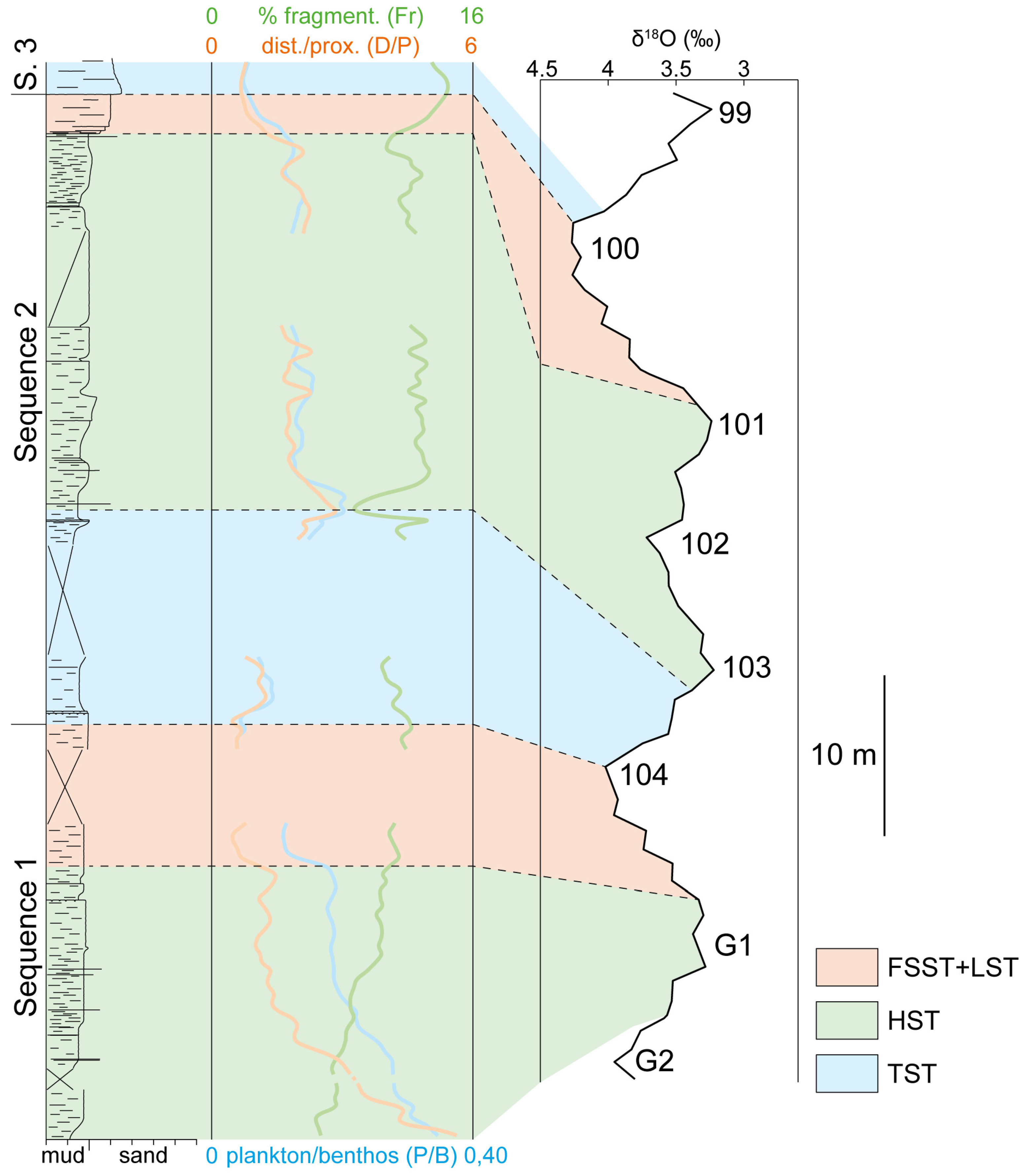
As for the control of the recognized cyclicity, the considered measured section corresponds to part of the Strongoli section of Capraro et al. [43], who documented warm–cold cycles ca. 40 m thick, based on the Sea Surface Temperature (SST) parameter, calculated by means of planktonic microforaminifera, and on the distribution of pollens. In particular, their cycles, which roughly coincide with the present higher rank sequences, were correlated to the Marine Isotopic Stages (MIS) based on a correlation between laminated layers occasionally found in the succession and the known Mediterranean sapropel layers. Based on the chronological framework by Capraro et al. [43], the HST of the higher rank Sequence 1, between 0 and 17 from the base of the measured section, would correlate to the MIS G1 interglacial (Figure 10), just predating the base of the Gelasian at ca. 2.58 Ma [70,71], whereas the HST of the higher rank Sequence 2, between ca. 39 and 62.5 m, would correlate to the MIS 103 interglacial (Figure 10), very close to the Piacenzian–Gelasian boundary. This implies that the inferred relative sea level fall associated with forced regression at the top of Sequence 1 would record the transition between MIS G1 and the MIS 104 glacial (Figure 10), whereas Capraro et al. [43] tentatively correlated part of the sharp-based shoreface above 62.5 m to the MIS 102 glacial. However, given the modest magnitude of MIS 102 [70,71], which contrasts with the marked relative sea level fall associated with the sharp-based shoreface, it is inferred that the latter records the transition between MIS 101 and the prominent MIS 100 glacial, whereas the modest MIS 102 and MIS 101 would correspond to the minor peaks of the D/P parameter found between 56.5 and 62.5 m or would be masked between 50.5 and 56.5 m (Figure 4, Figure 6 and Figure 10). It is not excluded that the relatively minor glacio-eustatic sea level fall associated with the MIS 103/102 transition was counteracted by local subsidence, as the associated rate of glacio-eustatic sea level fall was probably lower than that of the MIS G1/104 and MIS 101/100 transitions (Figure 10). It is therefore inferred that the HST of Sequence 2 would range between MIS 103 and MIS 101 (Figure 10).
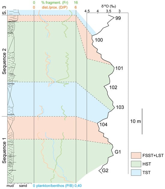
Figure 10.
Tentative correlation between the recognized higher rank sequences (see Figure 4) and Marine Isotopic Stages (MIS; see the δ18O curve, from Lisiecki and Raymo [71]), based on previous attributions by Capraro et al. [43] and the present hypothesis (see text). The δ18O curve is inferred to be a proxy for glacio-eustasy. Abbreviations: FSST: falling-stage systems tract; HST: highstand systems tract; TST: transgressive systems tract.
The present uncertainties suggest that the precise attribution of the recognized systems tracts to MISs remains tentative. However, if the studied succession accumulated between 2.7 and 2.5 Ma, across the Piacenzian–Gelasian boundary, the observed higher rank cyclicity would record the 41 kyr obliquity-paced period, which is known to characterize the latest Piacenzian to Gelasian times since ca. 2.8–2.7 Ma [71,72,73,74]. It should be noted, however, that in case the higher rank sequences include more MISs that are less easily recognizable, such as for the inferred situation of MIS 102 (Figure 10), their duration would be longer than that of the obliquity-paced cycles.
Given the considered age and the inferred Milankovitch control, the studied higher rank cyclicity is equivalent to that of the Wanganui Basin, New Zealand [68,72,73,75]. The Wanganui sequences are in fact controlled by the 41 kyr obliquity periodicity, and their scale is very similar to that of the higher rank sequences of the study area.
As for the control on the lower rank cyclicity, since higher rank sequences contain 10 or 11 lower rank ones, the latter should reflect a sub-Milankovitch cyclicity with a ca. 4 kyr periodicity (or longer in case higher rank sequences contain more MISs). Given the typical architecture of these lower rank sequences, consisting of alternating TSTs and HSTs (Figure 5 and Figure 6), they could be associated with climate changes leading to sediment supply variations in the basin and/or minor changes in the rate of relative sea level rise (e.g., [7]). The recognized lower rank sequences are similar to the Holocene millennial-scale parasequences of the Po Plain (Italy) by Amorosi et al. [76], which were inferred to have been controlled by minor relative sea level and/or sediment supply changes. The scale of the lower rank sequences is also similar to that of meter-scale sedimentary units composing shallow-marine deposits and considered as bedsets [77,78].
8. Conclusions
The integrated sedimentological and micropaleontological study of the middle shelf to lower shoreface succession of the late Piacenzian to early Gelasian Strongoli area has allowed us to document two orders of cyclicity of meter to decameter scale, characterized by both minor grain size and facies changes plus variable distributions of benthic microforaminifera assemblages. The recognition of sequence stratigraphic surfaces and transgressive–regressive trends at two different scales allowed us to define higher rank sequences up to ca. 40 m thick, composed of 10–11 lower rank sequences ca. 2.5 to 4 m thick. In particular, in such a relatively distal setting, minor transgressive and regressive trends, as well as MFSs and MRSs, are mainly recognizable by combining the curves of the D/P (ratio between distal and proximal benthic foraminifera) and Fr (percentage of fragmentation of benthic foraminifera) parameters, which are commonly accompanied by subtle grain size and facies changes usually reflecting modest shoreline shifts. Among the other micropaleontological parameters that have been considered, the P/B (plankton/benthos ratio) provides an indication of the bathymetric trend, with maxima that are generally later than the D/P maxima. The curves of the ‘abundance’ and ‘diversity’ parameters in some cases roughly follow the trend of the D/P curve, in others that of the P/B curve, but in general they provide a lower resolution and less certain indications.
The only surfaces found directly in the field are the RSME and the WRS, respectively, at the base and within lower shoreface deposits in the upper part of the measured section, and more subtle LFSs in the silty TSTs of lower rank sequences. While higher rank sequences can be documented in the whole measured section, the lower rank ones are only recognizable in lower shoreface and inner shelf settings.
The present data demonstrate that meter-scale, very high-frequency sequences such as the present lower rank ones, inferred to mainly reflect minor sediment supply changes and/or changes in the rate of relative sea level rise controlled by a sub-Milankovitch cyclicity, are still recognizable in inner shelf settings and tend to disappear toward middle shelf settings. This result is achievable by only combining the sedimentological evidence with the considered micropaleontological parameters, as this allows us to document almost cryptic sequences associated with minor shoreline shifts that otherwise would be poorly or not recognizable based on only outcrop and/or core data. The association of the recognized cyclicity with these minor shoreline shifts allows us to discriminate such meter-scale sequences from sedimentological cycles. The integration of sedimentological and micropaleontological data, therefore, represents a powerful tool for high-resolution sequence stratigraphic studies, which significantly increases our ability to investigate the stratigraphy cyclicity of sedimentary successions.
Supplementary Materials
The following supporting information can be downloaded at: https://www.mdpi.com/article/10.3390/geosciences15060210/s1, Table S1: Micropaleontological Table.
Author Contributions
Conceptualization, M.Z., M.C. and O.C.; methodology, M.Z. and M.C.; software, M.Z. and M.C.; validation, M.Z.; formal analysis, M.Z. and M.C.; investigation, M.Z., M.C. and O.C.; resources, M.Z. and M.C.; data curation, M.Z. and M.C.; writing—original draft preparation, M.Z.; writing—review and editing, M.Z., M.C. and O.C.; visualization, M.Z.; supervision, M.Z.; project administration, M.Z. All authors have read and agreed to the published version of the manuscript.
Funding
This research received no external funding.
Data Availability Statement
The original contributions presented in this study are included in the article/Supplementary Materials. Further inquiries can be directed to the corresponding author.
Conflicts of Interest
The authors declare no conflict of interest.
References
- Posamentier, H.W.; Allen, G.P. Siliciclastic sequence stratigraphy—Concepts and applications. SEPM Concepts Sedimentol. Paleontol. 1999, 7, 210. [Google Scholar]
- Catuneanu, O. Principles of Sequence Stratigraphy; Elsevier: Amsterdam, The Netherlands, 2006; p. 386. [Google Scholar]
- Catuneanu, O. Principles of Sequence Stratigraphy, 2nd ed.; Elsevier: Amsterdam, The Netherlands, 2022; p. 494. [Google Scholar]
- Zecchin, M.; Catuneanu, O. High-resolution sequence stratigraphy of clastic shelves I: Units and bounding surfaces. Mar. Pet. Geol. 2013, 39, 1–25. [Google Scholar] [CrossRef]
- Catuneanu, O. Scale in Sequence Stratigraphy. Mar. Pet. Geol. 2019, 106, 128–159. [Google Scholar] [CrossRef]
- Di Celma, C.; Cantalamessa, G. Sedimentology and high-frequency sequence stratigraphy of a forearc extensional basin: The Miocene Caleta Herradura Formation, Mejillones Peninsula, northern Chile. Sediment. Geol. 2007, 198, 29–52. [Google Scholar] [CrossRef]
- Zecchin, M.; Caffau, M.; Catuneanu, O. Recognizing maximum flooding surfaces in shallow-water deposits: An integrated sedimentological and micropaleontological approach (Crotone Basin, southern Italy). Mar. Pet. Geol. 2021, 133, 105225. [Google Scholar] [CrossRef]
- Zecchin, M.; Caffau, M.; Catuneanu, O. Identification of maximum flooding surfaces at different scales: The case of the Piacenzian to Gelasian Cutro Clay and Strongoli Sandstone (Crotone Basin, southern Italy). Mar. Pet. Geol. 2022, 146, 105971. [Google Scholar] [CrossRef]
- Zecchin, M.; Caffau, M.; Catuneanu, O. Zanclean to Gelasian high-frequency sequences of the Crotone Basin (southern Italy): Architectural variability and forcing mechanisms. Mar. Pet. Geol. 2024, 162, 106753. [Google Scholar] [CrossRef]
- Zecchin, M.; Catuneanu, O.; Caffau, M. High-resolution sequence stratigraphy of clastic shelves IX: Methods for recognizing maximum flooding conditions in shallow-marine settings. Mar. Pet. Geol. 2023, 156, 106468. [Google Scholar] [CrossRef]
- Amodio Morelli, L.; Bonardi, G.; Colonna, V.; Dietrich, D.; Giunta, G.; Ippolito, F.; Liguori, V.; Lorenzoni, S.; Paglionico, A.; Perrone, V.; et al. L’Arco Calabro-Peloritano nell’orogene Appenninico-Maghrebide. Mem. Soc. Geol. Ital. 1976, 17, 1–60. [Google Scholar]
- Van Dijk, J.P.; Bello, M.; Brancaleoni, G.P.; Cantarella, G.; Costa, V.; Frixa, A.; Golfetto, F.; Merlini, S.; Riva, M.; Torricelli, S.; et al. A regional structural model for the northern sector of the Calabrian Arc (southern Italy). Tectonophysics 2000, 324, 267–320. [Google Scholar] [CrossRef]
- Bonardi, G.; Cavazza, W.; Perrone, V.; Rossi, S. Calabria–Peloritani terrane and northern Ionian Sea. In Anatomy of an Orogen: The Apennines and Adjacent Mediterranean Basins; Vai, G.B., Martini, I.P., Eds.; Kluwer Academic Publishers: Bodmin, UK, 2001; pp. 287–306. [Google Scholar]
- Malinverno, A.; Ryan, W.B.F. Extension in the Tyrrhenian Sea and shortening in the Apennines as a result of arc migration driven by sinking of the lithosphere. Tectonics 1986, 5, 227–245. [Google Scholar] [CrossRef]
- Faccenna, C.; Becker, T.W.; Lucente, F.P.; Jolivet, L.; Rossetti, F. History of subduction and back-arc extension in the Central Mediterranean. Geophys. J. Int. 2001, 145, 809–820. [Google Scholar] [CrossRef]
- Faccenna, C.; Civetta, L.; D’Antonio, M.; Funiciello, F.; Margheriti, L.; Piromallo, C. Constraints on mantle circulation around the deforming Calabrian slab. Geophys. Res. Lett. 2005, 32, L06311. [Google Scholar] [CrossRef]
- Sartori, R. The Tyrrhenian back-arc basin and subduction of the Ionian lithosphere. Episodes 2003, 26, 217–221. [Google Scholar] [CrossRef]
- Guillaume, B.; Funiciello, F.; Faccenna, C.; Martinod, J.; Olivetti, V. Spreading pulses of the Tyrrhenian Sea during the narrowing of the Calabrian slab. Geology 2010, 38, 819–822. [Google Scholar] [CrossRef]
- Critelli, S. Provenance of Mesozoic to Cenozoic Circum-Mediterranean sandstones in relation to tectonic setting. Earth-Sci. Rev. 2018, 185, 624–648. [Google Scholar] [CrossRef]
- Tripodi, V.; Muto, F.; Brutto, F.; Perri, F.; Critelli, S. Neogene-quaternary evolution of the forearc and backarc regions between the Serre and Aspromonte Massifs, Calabria (southern Italy). Mar. Pet. Geol. 2018, 95, 328–343. [Google Scholar] [CrossRef]
- Critelli, S.; Martín-Martín, M. Provenance, Paleogeographic and paleotectonic interpretations of Oligocene-Lower Miocene sandstones of the western-central Mediterranean region: A review. J. Asian Earth Sci. 2022, 8, 100124. [Google Scholar] [CrossRef]
- Critelli, S.; Martín-Martín, M. History of western Tethys Ocean and the birth of the circum-Mediterranean orogeny as reflected by source-to-sink relations. Int. Geol. Rev. 2024, 66, 505–515. [Google Scholar] [CrossRef]
- Van Dijk, J.P.; Okkes, F.W.M. Neogene tectonostratigraphy and kinematics of Calabrian basins; implications for the geodynamics of the Central Mediterranean. Tectonophysics 1991, 196, 23–60. [Google Scholar] [CrossRef]
- Zecchin, M.; Massari, F.; Mellere, D.; Prosser, G. Anatomy and evolution of a Mediterranean-type fault bounded basin: The Lower Pliocene of the northern Crotone Basin (Southern Italy). Basin Res. 2004, 16, 117–143. [Google Scholar] [CrossRef]
- Roda, C. Distribuzione e facies dei sedimenti Neogenici nel Bacino Crotonese. Geol. Romana 1964, 3, 319–366. [Google Scholar]
- Van Dijk, J.P. Sequence stratigraphy, kinematics and dynamic geohistory of the Crotone Basin (Calabria arc, central mediterranean): An integrated approach. Mem. Soc. Geol. Ital. 1990, 44, 259–285. [Google Scholar]
- Zecchin, M.; Mellere, D.; Roda, C. Sequence stratigraphy and architectural variability in growth fault-bounded basin fills: A review of Plio-Pleistocene stratal units of the Crotone Basin, southern Italy. J. Geol. Soc. Lond. 2006, 163, 471–486. [Google Scholar] [CrossRef]
- Zecchin, M.; Caffau, M.; Civile, D.; Critelli, S.; Di Stefano, A.; Maniscalco, R.; Muto, F.; Sturiale, G.; Roda, C. The Plio-Pleistocene evolution of the Crotone Basin (southern Italy): Interplay between sedimentation, tectonics and eustasy in the frame of Calabrian Arc migration. Earth Sci. Rev. 2012, 115, 273–303. [Google Scholar] [CrossRef]
- Zecchin, M.; Civile, D.; Caffau, M.; Critelli, S.; Muto, F.; Mangano, G.; Ceramicola, S. Sedimentary evolution of the Neogene-Quaternary Crotone Basin (southern Italy) and relationships with large-scale tectonics: A sequence stratigraphic approach. Mar. Pet. Geol. 2020, 117, 104381. [Google Scholar] [CrossRef]
- Massari, F.; Prosser, G. Late Cenozoic tectono-stratigraphic sequences of the Crotone Basin: Insights on the geodynamic history of the Calabrian arc and Tyrrhenian Sea. Basin Res. 2013, 25, 26–51. [Google Scholar] [CrossRef]
- Criniti, S.; Borrelli, M.; Falsetta, E.; Civitelli, M.; Pugliese, E.; Arcuri, N. Sandstone petrology of the Crotone basin, Calabria (Italy) from well cores. Rend. Online Soc. Geol. Ital. 2023, 59, 64–70. [Google Scholar] [CrossRef]
- Mangano, G.; Zecchin, M.; Civile, D.; Critelli, S. Tectonic evolution of the Crotone Basin (central Mediterranean): The important role of two strike-slip fault zones. Mar. Pet. Geol. 2024, 163, 106769. [Google Scholar] [CrossRef]
- Gliozzi, E. I terrazzi del Pleistocene superiore della Penisola di Crotone (Calabria). Geol. Romana 1987, 26, 17–79. [Google Scholar]
- Cosentino, D.; Gliozzi, E.; Salvini, F. Brittle deformations in the Upper Pleistocene deposits of the Crotone Peninsula, Calabria, southern Italy. Tectonophysics 1989, 163, 205–217. [Google Scholar] [CrossRef]
- Cita, M.B. Studi sul Pliocene e sugli strati di passaggio dal Miocene al Pliocene. VIII. Planktonic foraminiferal biozonation of the Mediterranean Pliocene deep-sea record. A revision. Riv. Ital. Paleontol. Stratigr. 1975, 81, 527–544. [Google Scholar]
- Rio, D.; Raffi, I.; Villa, G. Pliocene-Pleistocene calcareous nannofossil distribution patterns in the Western Mediterranean. Proc. Ocean. Drill. Program Sci. Results 1990, 107, 513–533. [Google Scholar]
- Lourens, L.J.; Antonarakou, A.; Hilgen, F.J.; Van Hoof, A.A.M.; Vergnaud-Grazzini, C.; Zachariasse, W.J. Evaluation of the Plio-Pleistocene astronomical timescale. Paleoceanography 1996, 11, 391–413. [Google Scholar] [CrossRef]
- Raffi, I.; Backman, J.; Fornaciari, E.; Pälike, H.; Rio, D.; Lourens, L.; Hilgen, F. A review of calcareous nannofossil astrobiochronology encompassing the past 25 million years. Quat. Sci. Rev. 2006, 25, 3113–3137. [Google Scholar] [CrossRef]
- Reading, H.G.; Collinson, J.D. Clastic Coasts. In Sedimentary Environments; Processes, Facies and Stratigraphy; Reading, H.G., Ed.; Blackwell Science: Oxford, UK, 1996; pp. 154–231. [Google Scholar]
- Clifton, H.E. A reexamination of facies models for clastic shorelines. In Facies Models Revisited; Posamentier, H.W., Walker, R.G., Eds.; SEPM Special Publication: Tulsa, OK, USA, 2006; Volume 84, pp. 293–337. [Google Scholar]
- Zecchin, M.; Caffau, M.; Catuneanu, O.; Lenaz, D. Discrimination between wave-ravinement surfaces and bedset boundaries in Pliocene shallow-marine deposits, Crotone Basin, southern Italy: An integrated sedimentological, micropaleontological and mineralogical approach. Sedimentology 2017, 64, 1755–1791. [Google Scholar] [CrossRef]
- Loeblich, A.R.; Tappan, H. Foraminiferal Genera and Their Classification; Van Nostrand Reinhold Company: New York, NY, USA, 1987; p. 970. [Google Scholar]
- Capraro, L.; Consolaro, C.; Fornaciari, E.; Massari, F.; Rio, D. Chronology of the middle-upper Pliocene succession in the Strongoli area: Constraints on the geological evolution of the Crotone Basin (southern Italy). In Tectonics of the Western Mediterranean and North Africa; Moratti, G., Chalouan, A., Eds.; Geological Society Special Publication: London, UK, 2006; Volume 262, pp. 323–336. [Google Scholar]
- Jorissen, F.J. The distribution of benthic foraminifera in the Adriatic Sea. Mar. Micropaleontol. 1987, 12, 21–48. [Google Scholar] [CrossRef]
- Abbott, S.T. Foraminiferal paleobathymetry and mid-cycle architecture of mid-Pleistocene depositional sequences, Wanganui Basin, New Zealand. Palaios 1997, 12, 267–281. [Google Scholar] [CrossRef]
- Naish, T.R.; Kamp, P.J.J. Foraminiferal depth palaeoecology of Late Pliocene shelf sequences and system tracts, Wanganui Basin, New Zealand. Sediment. Geol. 1997, 110, 237–255. [Google Scholar] [CrossRef]
- Stefanelli, S. Benthic foraminiferal assemblages as tools for paleoenvironmental reconstruction of the early-middle Pleistocene Motalbano Jonico composite section. Boll. Soc. Paleontol. Ital. 2003, 42, 281–299. [Google Scholar]
- Mendes, I.; Gonzalez, R.; Dias, J.M.A.; Lobo, F.; Martins, V. Factors influencing recent benthic foraminifera distribution on the Guadiana shelf (Southwestern Iberia). Mar. Micropaleontol. 2004, 51, 171–192. [Google Scholar] [CrossRef]
- Morigi, C.; Jorissen, F.J.; Fraticelli, S.; Horton, B.P.; Principi, M.; Sabbatini, A.; Capotondi, L.; Curzi, P.V.; Negri, A. Benthic foraminiferal evidence for the formation of the Holocene mud-belt and bathymetrical evolution in the central Adriatic Sea. Mar. Micropaleontol. 2005, 57, 25–49. [Google Scholar] [CrossRef]
- Murray, J.W. Ecology and Applications of Benthic Foraminifera; Cambridge University Press: New York, NY, USA, 2006; p. 426. [Google Scholar]
- Phipps, M.D.; Kaminiski, M.A.; Aksu, A.E. Calcareous benthic foraminiferal biofacies along a depth transect on the southwestern marmara shelf (Turkey). Micropaleontology 2010, 56, 377–392. [Google Scholar] [CrossRef]
- Milker, Y.; Schmiedl, G. A taxonomic guide to modern benthic shelf foraminifera of the western Mediterranean Sea. Palaeontol. Electron. 2012, 15, 134. [Google Scholar] [CrossRef]
- Donnici, S.; Serandrei-Barbero, R. The benthic foraminiferal communities of the North Adriatic continental shelf. Mar. Micropaleontol. 2002, 44, 93–123. [Google Scholar] [CrossRef]
- Fillon, R.H. Biostratigraphy and condensed sections in deepwater settings. In Introduction to the Petroleum Geology of Deepwater Settings; Weimer, P., Slatt, R., Eds.; AAPG Studies in Geology 57, AAPG/Datapages Discovery Series; American Association of Petroleum Geologists: Tulsa, OK, USA, 2007; Volume 8. [Google Scholar]
- Gutiérrez Paredes, H.C.; Catuneanu, O.; Romano, U.H. Sequence stratigraphy of the Miocene section, southern Gulf of Mexico. Mar. Pet. Geol. 2017, 86, 711–732. [Google Scholar] [CrossRef]
- Jorissen, F.; Nardelli, M.P.; Almogi-Labin, A.; Barras, C.; Bergamin, L.; Bicchi, E.; El Kateb, A.; Ferraro, L.; Mary McGann, M.; Morigi, C.; et al. Developing Foram-AMBI for biomonitoring in the Mediterranean: Species assignments to ecological categories. Mar. Micropaleontol. 2018, 140, 33–45. [Google Scholar] [CrossRef]
- Hunt, D.; Tucker, M.E. Stranded parasequences and the forced regressive wedge systems tract: Deposition during base-level fall. Sediment. Geol. 1992, 81, 1–9. [Google Scholar] [CrossRef]
- Helland-Hansen, W.; Martinsen, O.J. Shoreline trajectories and sequences: Description of variable depositional-dip scenarios. J. Sediment. Res. 1996, 66, 670–688. [Google Scholar]
- Van Wagoner, J.C.; Mitchum, R.M.; Campion, K.M.; Rahmanian, V.D. Siliciclastic sequence stratigraphy in well logs, cores, and outcrops. AAPG Methods Explor. 1990, 7, 55. [Google Scholar]
- Abbott, S.T.; Carter, R.M. The sequence architecture of Mid-Pleistocene (c.1.1.-0.4Ma) cyclothems from New Zealand: Facies development during a Period of orbital control on sea-level cyclicity. In Orbital Forcing and Cyclic Sequences; De Boer, P.L., Smith, D.G., Eds.; IAS Special Publication: Hoboken, NJ, USA, 1994; Volume 19, pp. 367–394. [Google Scholar]
- Plint, A.G. Sharp-based shoreface sequences and offshore bars in the Cardium Formation of Alberta; their relationship to relative changes in sea level. In Sea Level Changes: An Integrated Approach; Wilgus, C.K., Hastings, B.S., Kendall, C.G.S.C., Posamentier, H.W., Ross, C.A., Van Wagoner, J.C., Eds.; SEPM Special Publication: Tulsa, OK, USA, 1988; Volume 42, pp. 357–370. [Google Scholar]
- Plint, A.G.; Nummedal, D. The falling stage systems tract: Recognition and importance in sequence stratigraphic analysis. In Sedimentary Responses to Forced Regressions; Hunt, D., Gawthorpe, R.L., Eds.; Geological Society Special Publication: Bath, UK, 2000; Volume 172, pp. 1–17. [Google Scholar]
- Swift, D.J. Coastal erosion and transgressive stratigraphy. J. Geol. 1968, 76, 444–456. [Google Scholar] [CrossRef]
- Demarest, J.M.; Kraft, J.C. Stratigraphic record of Quaternary sea levels: Implications for more ancient strata. In Sea-level Fluctuation and Coastal Evolution; Nummedal, D., Pilkey, O.H., Howard, J.D., Eds.; SEPM Special Publication: Tulsa, OK, USA, 1987; Volume 41, pp. 223–239. [Google Scholar]
- Nummedal, D.; Swift, D.J.P. Transgressive stratigraphy at sequence-bounding unconformities: Some principles derived from Holocene and Cretaceous examples. In Sea-Level Fluctuation and Coastal Evolution; Nummedal, D., Pilkey, O.H., Howard, J.D., Eds.; SEPM Special Publication: Tulsa, OK, USA, 1987; Volume 41, pp. 241–260. [Google Scholar]
- Zecchin, M.; Catuneanu, O.; Caffau, M. Wave-ravinement surfaces: Classification and key characteristics. Earth Sci. Rev. 2019, 188, 210–239. [Google Scholar] [CrossRef]
- Kidwell, S.M. Condensed deposits in siliciclastic sequences: Expected and observed features. In Cycles and Events in Stratigraphy; Einsele, G., Ricken, W., Seilacher, A., Eds.; Springer: Berlin/Heidelberg, Germany, 1991; pp. 682–695. [Google Scholar]
- Naish, T.R.; Kamp, P.J.J. Sequence stratigraphy of sixth-order (41 k.y.) Pliocene-Pleistocene cyclothems, Wanganui basin, New Zealand: A case for the regressive systems tract. Geol. Soc. Am. Bull. 1997, 109, 978–999. [Google Scholar] [CrossRef]
- Catuneanu, O.; Zecchin, M. High-resolution sequence stratigraphy of clastic shelves II: Controls on sequence development. Mar. Pet. Geol. 2013, 39, 26–38. [Google Scholar] [CrossRef]
- Shackleton, N.J.; Hall, M.A.; Pate, D. Pliocene stable isotope stratigraphy of ODP Site 846. Proc. Ocean. Drill. Program Sci. Results 1995, 138, 337–356. [Google Scholar]
- Lisiecki, L.E.; Raymo, M.E. A Pliocene-Pleistocene stack of 57 globally distributed benthic δ18O records. Paleoceanography 2005, 20, PA1003. [Google Scholar] [CrossRef]
- Grant, G.R.; Sefton, J.P.; Patterson, M.O.; Naish, T.R.; Dunbar, G.B.; Hayward, B.W.; Morgans, H.E.G.; Alloway, B.V.; Seward, D.; Tapia, C.A.; et al. Mid- to late Pliocene (3.3–2.6 Ma) global sea-level fluctuations recorded on a continental shelf transect, Whanganui Basin, New Zealand. Quat. Sci. Rev. 2018, 201, 241–260. [Google Scholar] [CrossRef]
- Grant, G.R.; Naish, T.R.; Dunbar, G.B.; Stocchi, P.; Kominz, M.A.; Kamp, P.J.J.; Tapia, C.A.; McKay, R.M.; Levy, R.H.; Patterson, M.O. The amplitude and origin of sea-level variability during the Pliocene epoch. Nature 2019, 574, 237–241. [Google Scholar] [CrossRef]
- Ochoa, D.; Sierro, F.J.; Hilgen, F.J.; Cortina, A.; Lofi, J.; Kouwenhoven, T.; Flores, J.-A. Origin and implications of orbital-induced sedimentary cyclicity in Pliocene well-logs of the Western Mediterranean. Mar. Geol. 2018, 403, 150–164. [Google Scholar] [CrossRef]
- Saul, G.; Naish, T.R.; Abbott, S.T.; Carter, R.M. Sedimentary cyclicity in the marine Pliocene-Pleistocene of the Wanganui basin (New Zealand): Sequence stratigraphic motifs characteristic of the past 2.5 m.y. GSA Bull. 1999, 111, 524–537. [Google Scholar] [CrossRef]
- Amorosi, A.; Centineo, M.C.; Colalongo, M.L.; Fiorini, F. Millennial-scale depositional cycles from the Holocene of the Po Plain, Italy. Mar. Geol. 2005, 222–223, 7–18. [Google Scholar] [CrossRef]
- Hampson, G.J.; Rodriguez, A.B.; Storms, J.E.A.; Johnson, H.D.; Meyer, C.T. Geomorphology and high-resolution stratigraphy of progradational wave-dominated shoreline deposits: Impact on reservoir-scale facies architecture. In Recent Advances in Models of Siliciclastic Shallow-Marine Stratigraphy; Hampson, G.J., Steel, R.J., Burgess, P.M., Dalrymple, R.W., Eds.; SEPM Special Publication: Tulsa, OK, USA, 2008; Volume 90, pp. 117–142. [Google Scholar]
- Ainsworth, R.B.; Vakarelov, B.K.; MacEachern, J.A.; Rarity, F.; Lane, T.I.; Nanson, R.A. Anatomy of a shoreline regression: Implications for the high-resolution stratigraphic architecture of deltas. J. Sediment. Res. 2017, 87, 425–459. [Google Scholar] [CrossRef]


Disclaimer/Publisher’s Note: The statements, opinions and data contained in all publications are solely those of the individual author(s) and contributor(s) and not of MDPI and/or the editor(s). MDPI and/or the editor(s) disclaim responsibility for any injury to people or property resulting from any ideas, methods, instructions or products referred to in the content. |
© 2025 by the authors. Licensee MDPI, Basel, Switzerland. This article is an open access article distributed under the terms and conditions of the Creative Commons Attribution (CC BY) license (https://creativecommons.org/licenses/by/4.0/).