
Comparison of Neural Network, Ordinary Kriging, and Inverse Distance Weighting Algorithms for Seismic and Well-Derived Depth Data: A Case Study in the Bjelovar Subdepression, Croatia


Abstract
1. Introduction
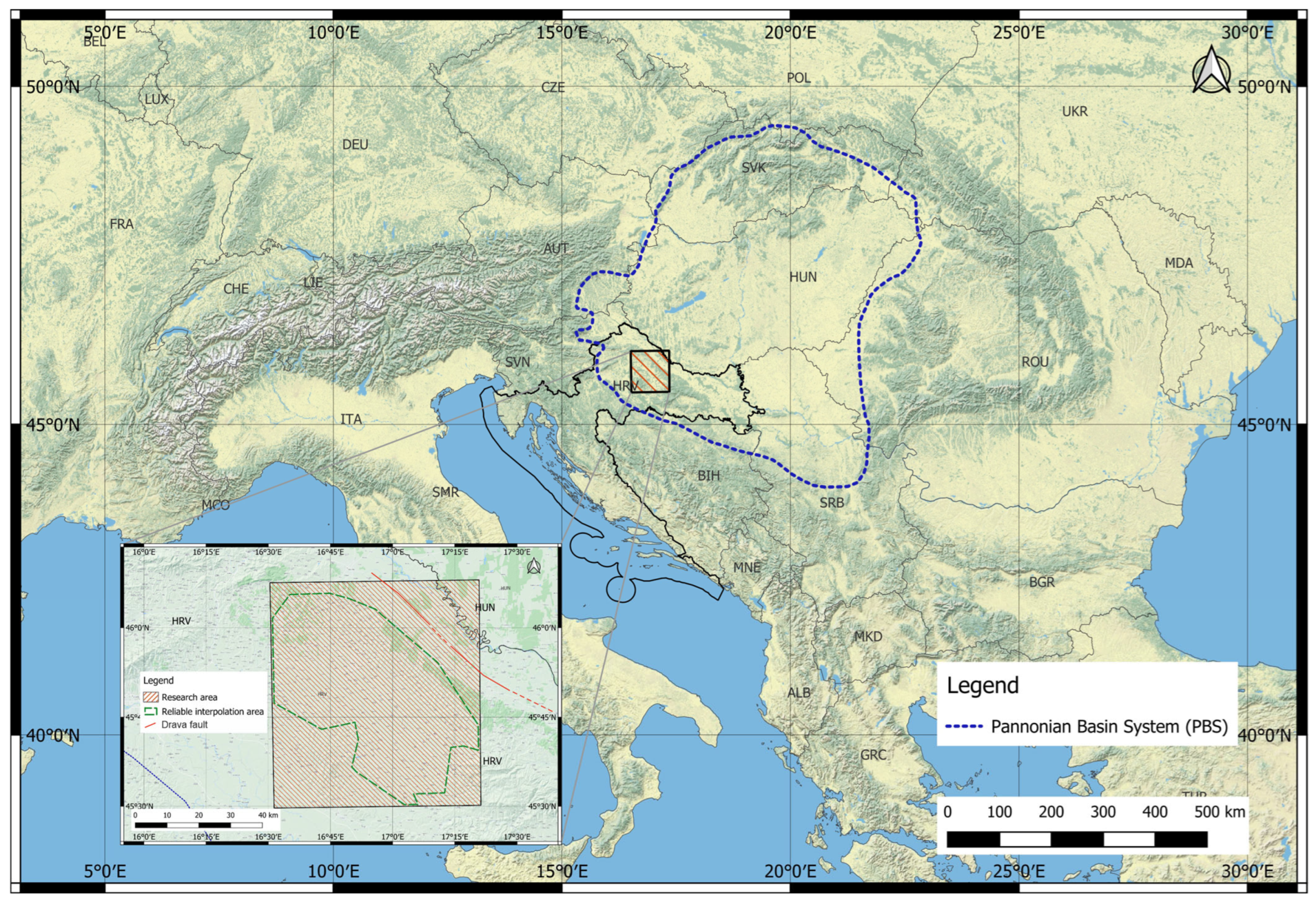
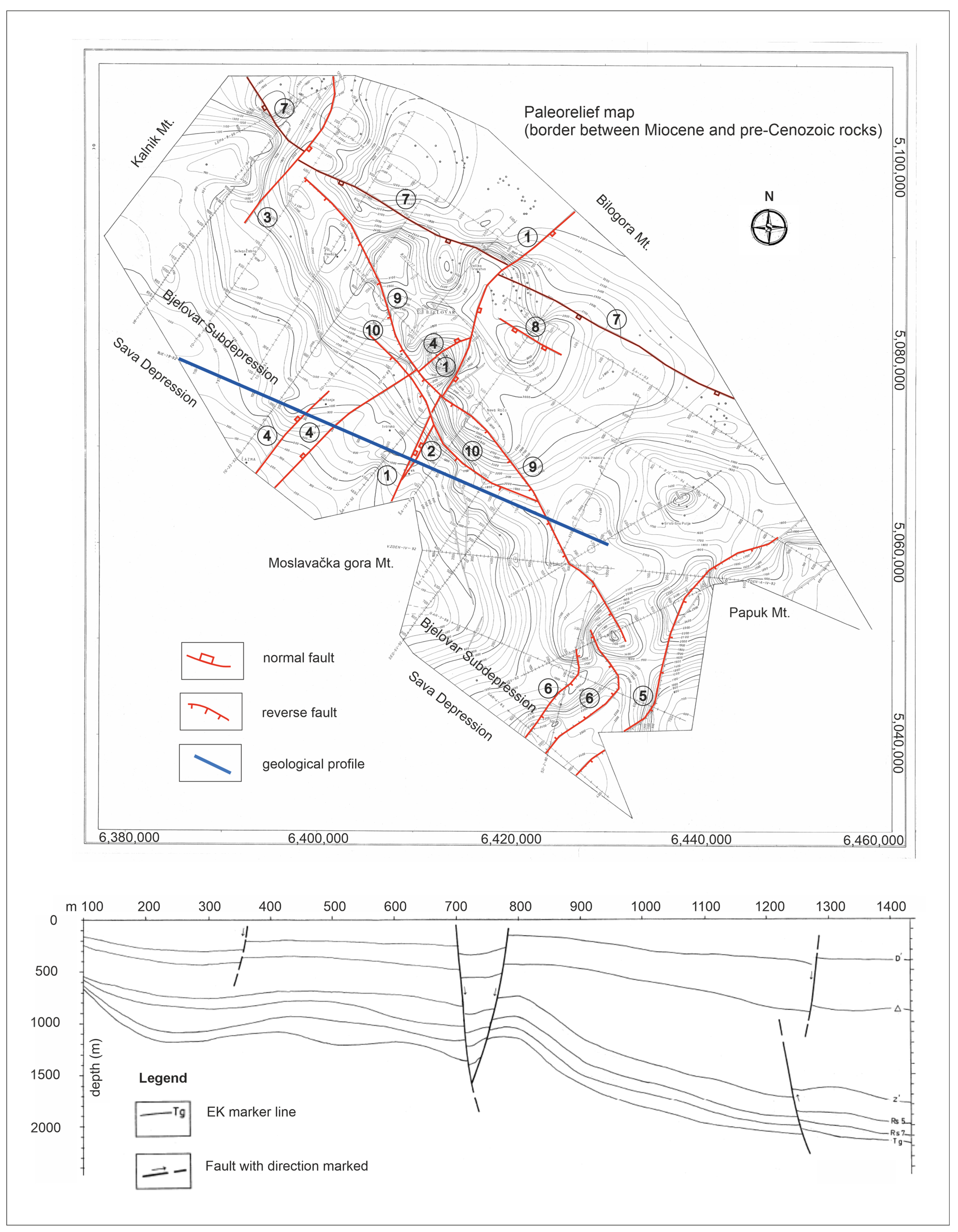
2. Geological Setting
3. Data and Methods
4. Results
4.1. Interpolation Methods
4.1.1. OK Maps
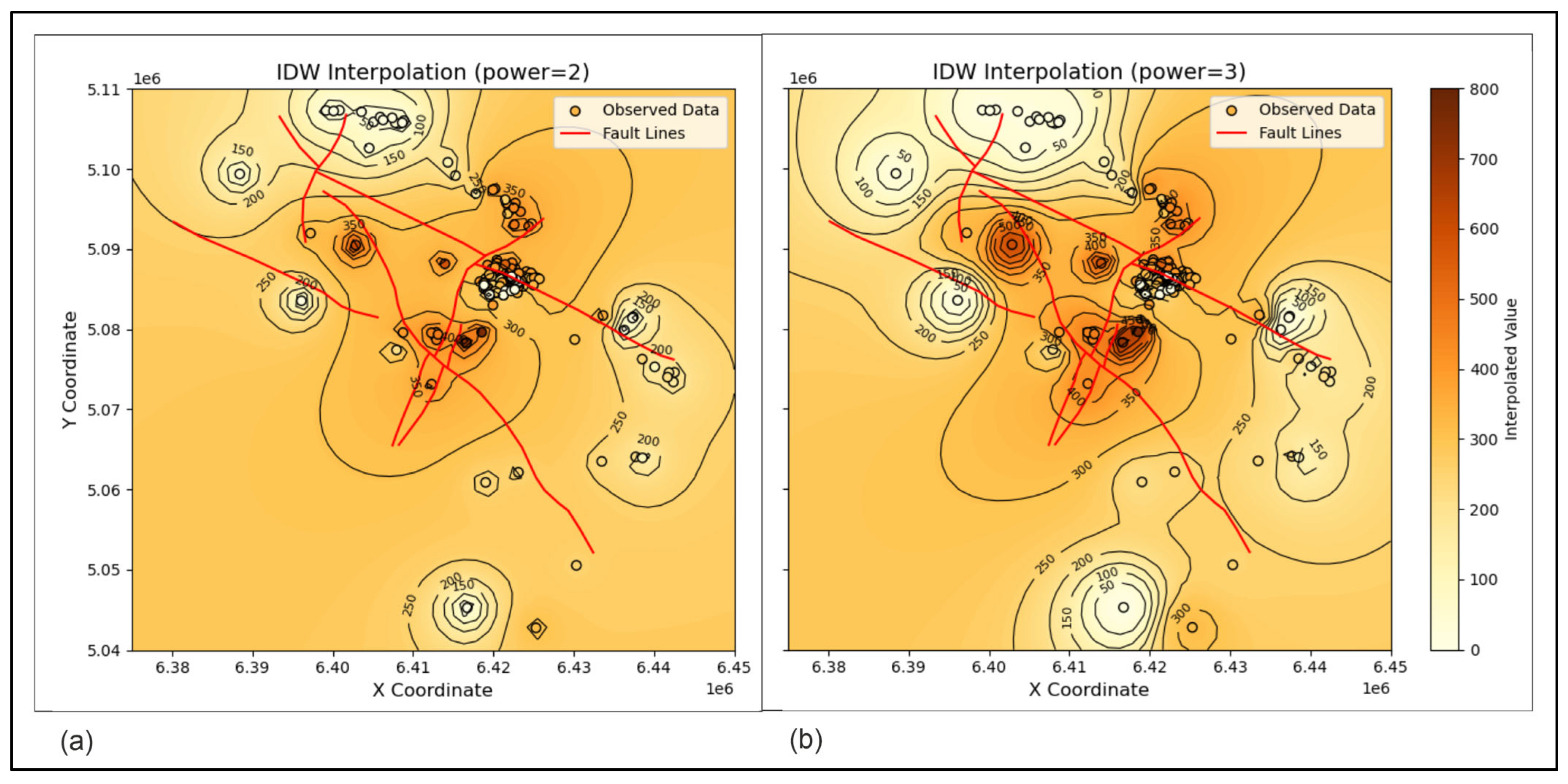
4.1.2. IDW Map
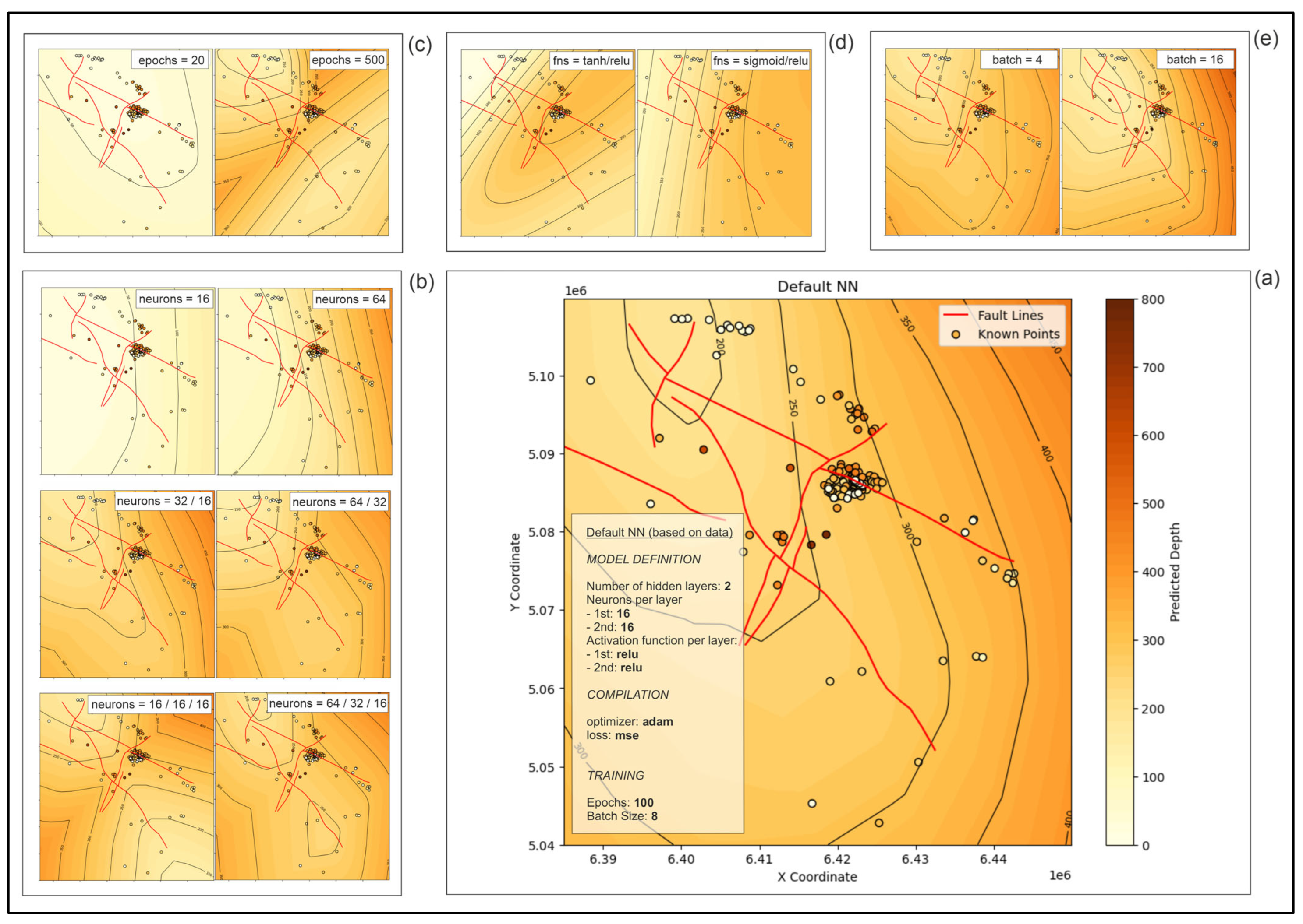
4.1.3. NN Maps
4.1.4. RF and XGB
5. Discussion
6. Conclusions
- It is well known that OK is dependent on the quality of variogram analysis, i.e., the number of data points and possible clustering. Here, we show that a variogram model, even one with a relatively high sill and occasional nugget effect, can be well fitted into a mapping model and surpass other methods applied to the presented area and datasets.
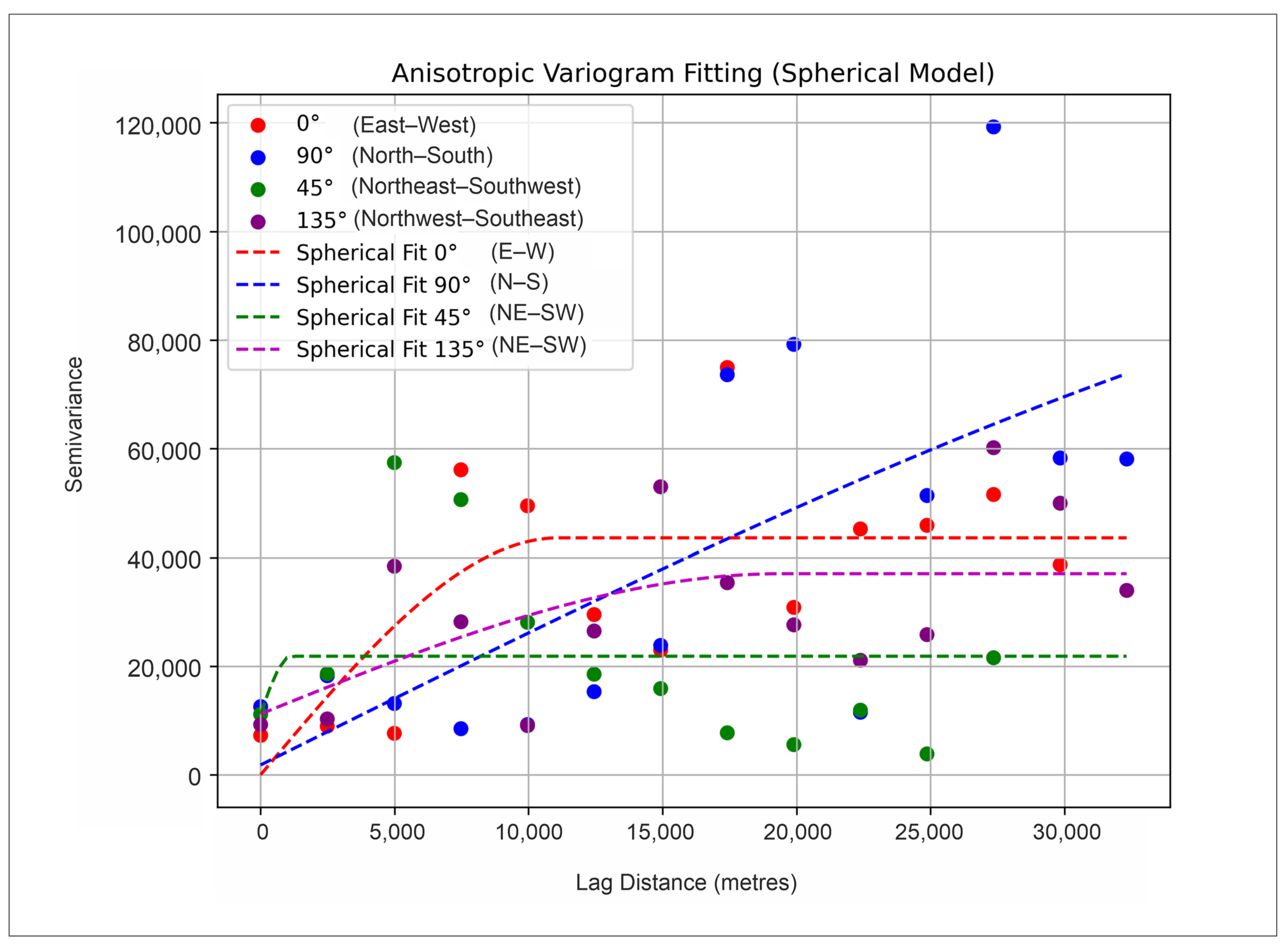
- A variogram model, with all included uncertainties, easily found spatial anisotropies, which had an origin in the structural shape (and, consequently, the tectonic zone’s directions, throws, and strike of depositional features) of the subdepression. Here, two variogram models representing anisotropy were chosen, one on the main subdepressional axis (135° NW-SE) and the other on the subordinate (45° NE-SW). As expected, the main axis variogram showed the best fit with the experimental points and the definition of range (about 15,000 m) and nugget (approx. 10,000).
- NN showed that it is a highly adjustable method for interpolation, where numerous hyperparameters can be adjusted. However, its high adjustability only makes the process more complex while geological representativeness still cannot be guaranteed or even achieved as in OK. In fact, in NN, hyperparameter optimization does help the statistical accuracy of a trained model, but it can be irrelevant to the geology of the area. That could be a pitfall in automated NN fitting. This is why our manually tuned models outperformed automatized tuners, such as Keras Tuner, because the best fitted model (the one with the smallest errors) in general follows geological and spatial facts and data.
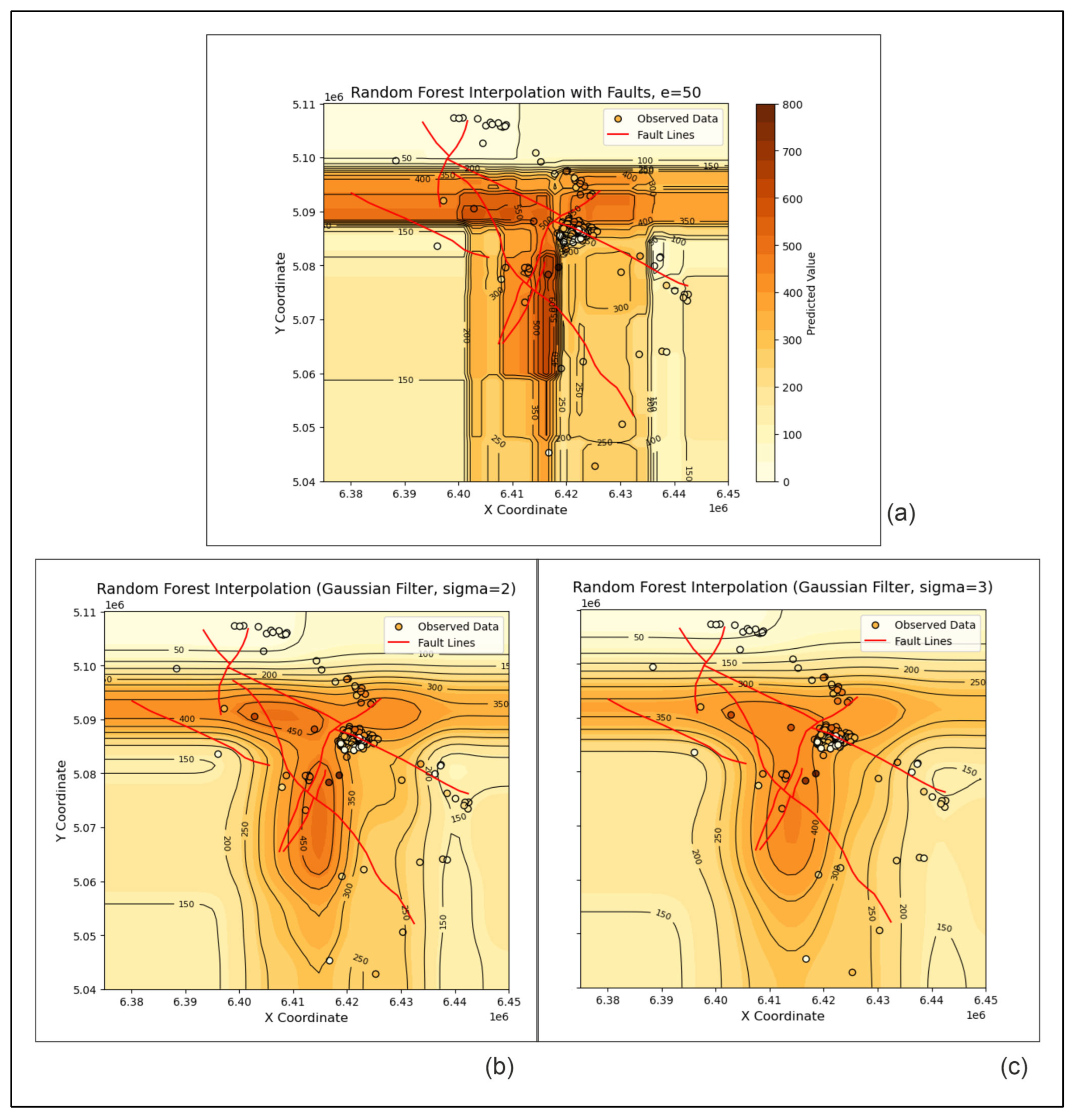
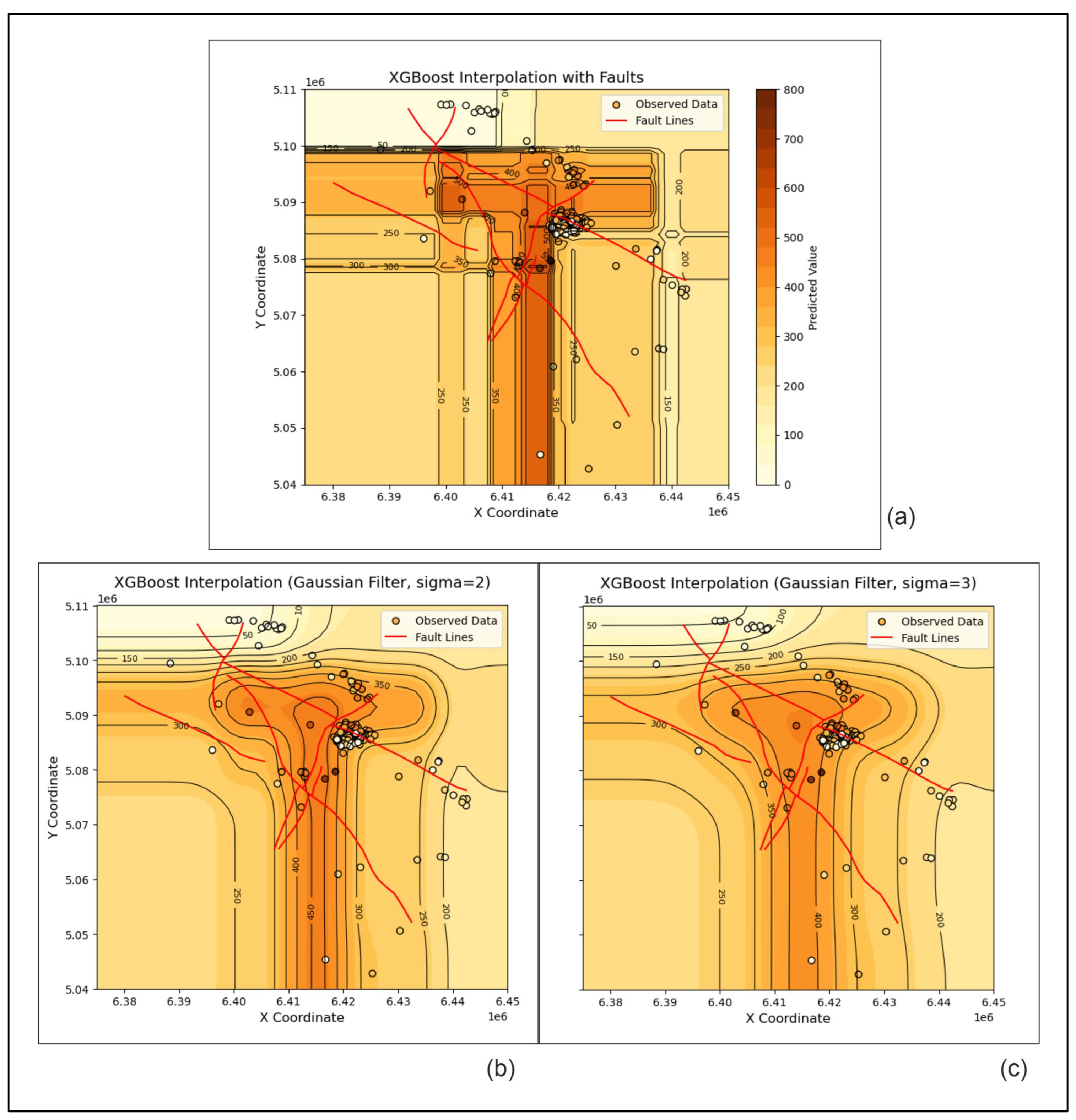
- IDW showed its strength as one of the classical interpolators with which the results are always located close to the top if several methods are compared. In contrast, the RF and XGB algorithms were found to be completely inapplicable to subsurface geological mapping, at least for the presented dataset and the area of the Bjelovar Subdepression.
- Even methods like OK, IDW, and NN will also perform poorly in the absence of enough numerous datasets, sometimes characterized with clustering. However, in the case of the analyzed dataset, any of those methods can be recommended for future mapping in the Bjelovar Subdepression and the entire CPBS (with similar datasets). The manually optimized NN could always be the second (supplementary) approach to OK (here, OK vs. NN RMSE was 100.53 vs. 122.15), used for checking the structural results and comparing cross-validation values, expecting similar or sometimes maybe slightly better values. If NN is considered to be time-consuming or unreliable for the fitting of certain parameters, the supporting method can be IDW, which is a simple and easily understandable algorithm in which the error is comparable with that of the advanced NN (here, NN vs. IDW RMSE was 123.66 vs. 122.15).
- Neural algorithms in mapping are still rarely used, but here, we gave an example of such an application based on real subsurface geological data collected in clastics. Secondly, but equally importantly, here it was shown that even in such an abundant dataset, although partially clustered, the kriging method is still an option that could surpass a neural algorithm with several modifications of its parameters.
- Moreover, OK is better than the machine learning RF and XGB algorithms, which are completely unsuitable for this purpose. This was not surprising because kriging is a well-established method exclusively used for interpolation. In contrast, NN and machine learning algorithms are used in so many fields that their algorithms, including the fitting of hyperparameters in NN, simply cannot be the best solution for all types of applications.
- These novelties, mentioned in the previous two points, can be considered as especially important for other researchers with experience in geological mapping.
- It is worth mentioning that the kriging algorithm intrinsically includes uncertainties (like kriging variance but also uncertainties linked to deterministic estimation in each grid cell). As the kriged map was the best option presented in this work, it is meaningful to assume that future improvement of this work should move in the direction of mapping using stochastic Gaussian simulation, which can be investigated as a better option than the fitting of NNs, whether automatically or using expert opinions.
Supplementary Materials
Author Contributions
Funding
Data Availability Statement
Acknowledgments
Conflicts of Interest
Abbreviations
| OK | Ordinary kriging |
| IDW | Inverse distance weighting |
| NN | Neural network |
| RF | Random forest |
| XGB | Extreme gradient boosting |
| CV | Cross-validation |
| MAE | Mean Absolute Error |
| MSE | Mean Squared Error |
| RMSE | Root Mean Squared Error |
References
- Chen, P. A Rapid Supervised Learning Neural Network for Function Interpolation and Approximation. IEEE Trans. Neural Netw. 1996, 7, 1220–1230. [Google Scholar] [CrossRef]
- Ripley, B.D. Spatial Statistics; John Wiley & Sons: New York, NY, USA, 1981. [Google Scholar]
- Rosenblatt, F. The Perceptron: A Perceiving and Recognizing Automaton; Report; Project PARA; Cornell Aeronautical Laboratory: Ithaca, NY, USA, 1957; 58p. [Google Scholar]
- Achite, M.; Tsangaratos, P.; Pellicone, G.; Mohammadi, B.; Caloiero, T. Application of Multiple Spatial Interpolation Approaches to Annual Rainfall Data in the Wadi Cheliff Basin (North Algeria). Ain Shams Eng. J. 2024, 15, 102578. [Google Scholar] [CrossRef]
- Malvić, T. Geological Maps of Neogene Sediments in the Bjelovar Subdepression (Northern Croatia). J. Maps 2011, 7, 304–317. [Google Scholar]
- Špelić, M.; Malvić, T.; Saraf, V.; Zalović, M. Remapping of Depth of E-Log Markers between Neogene Basement and Lower/Upper Pannonian Border in the Bjelovar Subdepression. J. Maps 2016, 12, 45–52. [Google Scholar] [CrossRef]
- Kiš, I.M. Comparison of Ordinary and Universal Kriging Interpolation Techniques on a Depth Variable (a Case of Linear Spatial Trend), Case Study of the Šandrovac Field. Rud.-Geol.-Naft. Zb. 2016, 31, 41–58. [Google Scholar] [CrossRef]
- Latifovic, R.; Pouliot, D.; Campbell, J. Assessment of Convolution Neural Networks for Surficial Geology Mapping in the South Rae Geological Region, Northwest Territories, Canada. Remote Sens. 2018, 10, 307. [Google Scholar] [CrossRef]
- Shirmard, H.; Farahbakhsh, E.; Heidari, E.; Pour, A.B.; Pradhan, B.; Müller, D.; Chandra, R. A Comparative Study of Convolutional Neural Networks and Conventional Machine Learning Models for Lithological Mapping Using Remote Sensing Data. Remote Sens. 2022, 14, 819. [Google Scholar] [CrossRef]
- Malvić, T.; Velić, J.; Horváth, J.; Cvetković, M. Neural Networks in Petroleum Geology as Interpretation Tools. Cent. Eur. Geol. 2010, 53, 97–115. [Google Scholar] [CrossRef]
- Krige, D.G. A Statistical Approach to Some Basic Mine Valuation Problems on the Witwatersrand. J. Chem. Metall. Min. Soc. S. Afr. 1952, 52, 119–139. [Google Scholar] [CrossRef]
- Georges, M.; Fernand, B. Traité de Géostatistique Appliquée; Bureau de recherches géologiques et minières; Tome, I., Ed.; Technip: Paris, France, 1962. [Google Scholar]
- Georges, M. Principles of Geostatistics. Econ. Geol. 1963, 58, 1246–1266. [Google Scholar]
- Matheron, G. Les Variables Régionalisées et Leur Estimation. Une Application de La Théorie Des Fonctions Aléatoires Aux Sciences de La Nature; Masson: Échandens, Switzerland, 1965. [Google Scholar]
- Journel, A.G.; Huijbregts, C.J. Mining Geostatistics; Academic Press: Cambridge, MA, USA, 1978. [Google Scholar]
- Isaaks, E.; Srivastava, R. An Introduction to Applied Geostatistics; Oxford University Press Inc.: Oxford, UK, 1989. [Google Scholar]
- Cressie, N. The Origins of Kriging. Math. Geol. 1990, 22, 239–252. [Google Scholar] [CrossRef]
- Deutsch, C.V.; Journel, A.G. GSLIB: Geostatistical Software Library and User’s Guide (Applied Geostatistics Series), 2nd ed.; Oxford University Press: Oxford, UK, 1997. [Google Scholar]
- Rosenblatt, F. The Perceptron: A Probabilistic Model for Information Storage and Organization in the Brain. Psychol. Rev. 1958, 65, 386–408. [Google Scholar] [CrossRef] [PubMed]
- Riedmiller, M.; Braun, H. A Direct Adaptive Method for Faster Backpropagation Learning: The RPROP Algorithm. In Proceedings of the IEEE International Conference on Neural Networks, Nagoya, Japan, 25–29 October 1993; pp. 586–591. [Google Scholar]
- Srivardhan, V. Adaptive Boosting of Random Forest Algorithm for Automatic Petrophysical Interpretation of Well Logs. Acta Geod. Geophys. 2022, 57, 495–508. [Google Scholar] [CrossRef]
- Feng, R.; Grana, D.; Balling, N. Imputation of Missing Well Log Data by Random Forest and Its Uncertainty Analysis. Comput. Geosci. 2021, 152, 104763. [Google Scholar] [CrossRef]
- Behnamian, A.; Millard, K.; Banks, S.N.; White, L.; Richardson, M.; Pasher, J. A Systematic Approach for Variable Selection with Random Forests: Achieving Stable Variable Importance Values. IEEE Geosci. Remote Sens. Lett. 2017, 14, 1988–1992. [Google Scholar] [CrossRef]
- Micić Ponjiger, T.; Šešum, S.; Naugolnov, M.V.; Pilipenko, O. Lithology Classification by Depositional Environment and Well Log Data Using XGBoost Algorithm. In Proceedings of the Data Science in Oil and Gas 2021, DSOG 2021, Online, 4–6 August 2021; EAGE Publishing BV: Utrecht, The Netherlands, 2021. [Google Scholar]
- Kranjec, V.; Prelogović, E.; Hernitz, Z.; Blašković, I. O litofacijelnim odnosima mlađih neogenskih i kvartarnih sedimenata u širem području Bilogore (sjeverna Hrvatska). Geološki Vjesn. 1971, 24, 47–55. [Google Scholar]
- Malvić, T. Strukturni i Tektonski Odnosi te Značajke Ugljikovodika Širega Područja Naftnoga Polja Galovac-Pavljani; Faculty of Mining, Geology and Petroleum Engineering, University of Zagreb: Zagreb, Croatia, 1998. [Google Scholar]
- Malvić, T. Ležišne vode naftnoga polja Galovac-Pavljani. Hrvat. Vode 1999, 7, 139–148. [Google Scholar]
- Pletikapić, V. Naftoplinonosnost Dravske potoline. Nafta 1964, 9, 250–254. [Google Scholar]
- Pletikapić, V.; Gjetvaj, I.; Jurković, M.; Urbiha, H.; Hrnčić, L. Geologija i naftoplinonosnost Dravske potoline. Geološki Vjesn. 1964, 17, 49–78. [Google Scholar]
- Prelogović, E.; Hernitz, Z.; Blašković, I. Primjena morfometrijskih metoda u rješavanju strukturno-tektonskih odnosa na području Bilogore (sjev. Hrvatska). Geološki Vjesn. 1969, 22, 525–531. [Google Scholar]
- Magdalenić, Z.; Novosel, S. Tumač za List Bjelovar—Sedimentnopetrografske Karakteristike Nevezanih Stijena Neogena i Kvartara; Savezni geoloski zavod, Beograd. 1986. Available online: https://www.hgi-cgs.hr/wp-content/uploads/2020/07/Bjelovar.pdf (accessed on 11 May 2025).
- Jamičić, D. Osnovna Geološka Karta M 1:100.000—List Daruvar; Geološki Zavod Zagreb: Zagreb, Croatia, 1988. [Google Scholar]
- Jamičić, D.; Vragović, M.; Matičec, D. Osnovna Geološka Karta SFRJ 1:100 000, Tumač za List Daruvar; Geološki Zavod Srbije: Beograd, Serbia, 1988. [Google Scholar]
- Malvić, T. Naftnogeološki Odnosi i Vjerojatnost Pronalaska Novih Zaliha Ugljikovodika u Bjelovarskoj Uleknini [Oil-Geological Relations and Probability of Discovering New Hydrocarbon Reserves in the Bjelovar Sag]; Faculty of Mining, Geology and Petroleum Engineering, University of Zagreb: Zagreb, Croatia, 2003. [Google Scholar]
- Royden, L. Late Cenozoic Tectonics of the Pannonian Basin System. In The Pannonian Basin: A Study in Basin Evolution. AAPG Memoir 45; Royden, L.H., Horvath, F., Eds.; AAPG: Tulsa, OK, USA, 1988. [Google Scholar]
- Rögl, F. Palaeogeographic Considerations for Mediterranean and Paratethys Seaways (Oligocene to Miocene). Ann. Des Naturhistorischen Mus. 1998, 99, 279–310. [Google Scholar]
- Rögl, F. Stratigraphic Correlation of the Paratethys Oligocene and Miocene. Mitteilungen Ges. Geol. Bergbaustud. Osterr. 1996, 41, 65–73. [Google Scholar]
- Rögl, F.; Steininger, F. Neogene, Parathetys, Mediterranean and Indo-Pacific Seaways. In Fossil and Climate; Brenchey, P., Ed.; Wiley and Sons: Hoboken, NJ, USA, 1984; pp. 171–200. [Google Scholar]
- Steininger, F.; Rögl, F.; Müller, C. Chronostratigraphie Und Neostratotypen: Miozän Der Zentralen Paratethys, Band VI; Schweizerbart Science Publishers: Stuttgart, Germany, 1978. [Google Scholar]
- Piller, W.E.; Harzhauser, M.; Mandic, O. Miocene Central Paratethys Stratigraphy—Current Status and Future Directions. Stratigraphy 2007, 4, 151–168. [Google Scholar] [CrossRef]
- Malvić, T.; Velić, J. Neogene Tectonics in Croatian Part of the Pannonian Basin and Reflectance in Hydrocarbon Accumulations; InTech: London, UK, 2011. [Google Scholar]
- Haq, B.U.; van Eysinga, F.W.B. Geological Time Table, 5th ed.; Elsevier Science Ltd.: London, UK, 1998. [Google Scholar]
- Pavelić, D. Tectonostratigraphic Model for the North Croatian and North Bosnian Sector of the Miocene Pannonian Basin System. Basin Res. 2001, 13, 359–376. [Google Scholar] [CrossRef]
- Pavelić, D.; Miknic, M.; Šrlat, M.S. Early To Middle Miocene Facies Succession in Lacustrine and Marine Environments on the Southwestern Margin of the Pannonian Basin System (Croatia). Geol. Carpathica 1998, 49, 433–443. [Google Scholar]
- Prelogović, E. Neotektonska karta SR Hrvatske. Geološki Vjesn. 1975, 28, 97–108. [Google Scholar]
- Malvić, T. Regional Geological Settings and Hydrocarbon Potential of Bjelovar Sag (Subdepression), R. Croatia. Naft. 2004, 55, 273–288. [Google Scholar]
- National Spatial Data Infrastructure (NIPP). Coordinate Reference System. Available online: https://www.nipp.hr/default.aspx?id=3207 (accessed on 10 February 2025).
- The Pandas Development Team. pandas-dev/pandas: Pandas. 2020. Available online: https://zenodo.org/records/13819579 (accessed on 11 May 2025). [CrossRef]
- He, Y.; Chen, D.; Li, B.G.; Huang, Y.F.; Hu, K.L.; Li, Y.; Willett, I.R. Sequential Indicator Simulation and Indicator Kriging Estimation of 3-Dimensional Soil Textures. Soil Res. 2009, 47, 622. [Google Scholar] [CrossRef]
- Malvić, T. Primjena Geostatistike u Analizi Geoloških Podataka; INA—Industrija Nafte: Zagreb, Croatia, 2008. [Google Scholar]
- Murphy, B.; Yurchak, R.; Müller, S. GeoStat-Framework/PyKrige; V1.7.2; UFZ Leipzig: Leipzig, Germany, 2024. [Google Scholar]
- Pedregosa, F.; Michel, V.; Grisel, O.; Blondel, M.; Prettenhofer, P.; Weiss, R.; Dubourg, V.; Vanderplas, J.; Passos, A.; Cournapeau, D.; et al. Scikit-Learn: Machine Learning in Python. J. Mach. Learn. Res. 2011, 12, 2825–2830. [Google Scholar]
- Zhao, F.H.; Zhu, A.X.; Qin, C.Z. Spatial Distribution Pattern Analysis Using Variograms over Geographic and Feature Space. Geo-Spat. Inf. Sci. 2024, 1–15. [Google Scholar] [CrossRef]
- Nansen, C. Use of Variogram Parameters in Analysis of Hyperspectral Imaging Data Acquired from Dual-Stressed Crop Leaves. Remote Sens. 2012, 4, 180–193. [Google Scholar] [CrossRef]
- MacCormack, K.; Arnaud, E.; Parker, B.L. Using a Multiple Variogram Approach to Improve the Accuracy of Subsurface Geological Models. Can. J. Earth Sci. 2018, 55, 786–801. [Google Scholar] [CrossRef]
- Malvić, T.; Ivšinović, J.; Velić, J.; Sremac, J.; Barudžija, U. Application of the Modified Shepard’s Method (MSM): A Case Study with the Interpolation of Neogene Reservoir Variables in Northern Croatia. Stats 2020, 3, 68–83. [Google Scholar] [CrossRef]
- McDonald, A. Data Quality Considerations for Petrophysical Machine-Learning Models. Petrophysics 2021, 62, 585–613. [Google Scholar]
- Bahri, Y.; Dyer, E.; Kaplan, J.; Lee, J.; Sharma, U. Explaining Neural Scaling Laws. Proc. Natl. Acad. Sci. USA 2024, 121, e2311878121. [Google Scholar] [CrossRef]
- O’Malley, T.; Bursztein, E.; Long, J.; Chollet, F.; Jin, H.; Invernizzi, L. Keras Tuner. 2019. Available online: https://github.com/keras-team/keras-tuner (accessed on 12 February 2025).
- Madison Schott Random Forest Algorithm for Machine Learning. Available online: https://medium.com/capital-one-tech/random-forest-algorithm-for-machine-learning-c4b2c8cc9feb (accessed on 11 February 2025).
- Li, Z.; Lu, T.; Yu, K.; Wang, J. Interpolation of GNSS Position Time Series Using GBDT, XGBoost, and RF Machine Learning Algorithms and Models Error Analysis. Remote Sens. 2023, 15, 4374. [Google Scholar] [CrossRef]
- Chen, T.; Guestrin, C. XGBoost: A Scalable Tree Boost. System; Association for Computing Machinery: New York, NY, USA, 2016. [Google Scholar] [CrossRef]
- Sun, L. Application and Improvement of Xgboost Algorithm Based on Multiple Parameter Optimization Strategy. In Proceedings of the 2020 5th International Conference on Mechanical, Control and Computer Engineering (ICMCCE), Harbin, China, 25–27 December 2020; Institute of Electrical and Electronics Engineers Inc.: Piscataway, NJ, USA, 2020; pp. 1822–1825. [Google Scholar]
- Krkač, M.; Bernat Gazibara, S.; Arbanas, Ž.; Sečanj, M.; Mihalić Arbanas, S. A Comparative Study of Random Forests and Multiple Linear Regression in the Prediction of Landslide Velocity. Landslides 2020, 17, 2515–2531. [Google Scholar] [CrossRef]
- Barudžija, U.; Ivšinović, J.; Malvić, T. Selection of the Value of the Power Distance Exponent for Mapping with the Inverse Distance Weighting Method—Application in Subsurface Porosity Mapping, Northern Croatia Neogene. Geosciences 2024, 14, 155. [Google Scholar] [CrossRef]
- Pang, B.; Nijkamp, E.; Wu, Y.N. Deep Learning With TensorFlow: A Review. J. Educ. Behav. Stat. 2020, 45, 227–248. [Google Scholar] [CrossRef]
- Abadi, M.; Agarwal, A.; Barham, P.; Brevdo, E.; Chen, Z.; Citro, C.; Corrado, G.S.; Davis, A.; Dean, J.; Devin, M.; et al. TensorFlow: Large-Scale Machine Learning on Heterogeneous Distributed Systems. arXiv 2016, arXiv:1603.04467. [Google Scholar]
- Ravichandiran, S. Hands-On Deep Learning Algorithms with Python; Packt Publishing: Birmingham, UK, 2019; ISBN 978-1-78934-415-8. [Google Scholar]
- Lichtner-Bajjaoui, A.; Vives, J. A Mathematical Introduction to Neural Networks. Master’s Thesis, Universitat de Barcelona, Barcelona, Spain, 2021. [Google Scholar]
- Obuchowski, A. Understanding Neural Networks 2: The Math of Neural Networks in 3 Equations. Available online: https://becominghuman.ai/understanding-neural-networks-2-the-math-of-neural-networks-in-3-equations-6085fd3f09df (accessed on 31 January 2025).
- Saravanan, D.K. A Gentle Introduction To Math Behind Neural Networks. Available online: https://towardsdatascience.com/introduction-to-math-behind-neural-networks-e8b60dbbdeba (accessed on 31 January 2025).
- Schiavo, M. Spatial modeling of the water table and its historical variations in Northeastern Italy via a geostatistical approach. Groundw. Sustain. Dev. 2024, 25, 101186. [Google Scholar] [CrossRef]
- Remy, N.; Boucher, A.; Wu, J. Applied Geostatistics with SGeMS: A User’s Guide; Cambridge University Press: Cambridge, UK, 2009; 288p, ISBN 9780521514149. [Google Scholar]
- Schiavo, M. Numerical impact of variable volumes of Monte Carlo simulations of heterogeneous conductivity fields in groundwater models. J. Hydrol. 2024, 634, 131072. [Google Scholar] [CrossRef]
- Mälicke, M.; Guadagnini, A.; Zehe, E. SciKit-GStat Uncertainty: A software extension to cope with uncertain geostatistical estimates. Spat. Stat. 2023, 54, 100737. [Google Scholar] [CrossRef]


| Pre-Cenozoic–Miocene | Sarmatian–Early Pannonian | Early–Late Pannonian | Late Pannonian–Early Pontian | Early–Late Pontian | Late Pontian–Pliocene | |
|---|---|---|---|---|---|---|
| (16.4 Ma) | (11.5 Ma) | (9.3 Ma) | (7.1 Ma) | (6.3 Ma) | (5.6 Ma) | |
| Transverse normal faults (NE-SW) | ||||||
| (1) Primary normal | 300 | 100 | 100–200 | 100 | 100 | 50 |
| (2) Secondary normal | 100 | 100 | 100 | - | - | - |
| (3) Western | 150 | 100 | 100 | 50 | 50 | 50 |
| (4) Štefanje | 50 | 50 | 50 | 50 | 50 | 50 |
| (5) Eastern marginal | 100 | 100 | Unconf. | Unconf. | 100 | 50 |
| (6) Uljanik | 100 | 100 | Unconf. | Unconf. | 100 | 50–100 |
| Diagonal faults (WNW-ESE) | ||||||
| (7) Bilogora | 200 | 100 | 100–200 | 100 | 50 | 100 |
| (8) Šandrovac-Ciglena | 50 | 100 | 100–200 | 50 | 50 | 50 |
| (9) Primary reverse | 200 | 100 | 100 | 100 | 100 | 50 |
| (10) Secondary reverse | 200 | 100 | 50–100 | 100 | - | - |
| Stage | Hyperparameter | Value |
|---|---|---|
| Model definition | Number of hidden layers | 2 |
| Neurons per layer | 16 | |
| 16 | ||
| Activation function | ‘relu’ | |
| ‘relu’ | ||
| Model compilation | Optimizer | ‘adam’ |
| Loss function | ‘mse’ | |
| Metrics | ||
| Model training (fitting) | Epochs | 100 |
| Batch size | 8 | |
| Validation split | 0.2 | |
| Callbacks | - |
| Algorithm | CV (Cross-Validation) | MAE (Mean Absolute Error) | MSE (Mean Square Error) | RMSE (Root Mean Square Error) |
|---|---|---|---|---|
| OK | k-fold = 5 | 66.69 | 10,106.45 | 100.53 |
| IDW | 82.21 | 14,921.11 | 122.15 | |
| Manually optimized NN | 87.85 | 15,290.94 | 123.66 | |
| Automatically optimized NN | 110.94 | 20,821 | 144.29 |
| Method | Strengths | Weaknesses | Best Use Case |
|---|---|---|---|
| OK | - Well captures spatial correlation in the larger datasets; - Provides uncertainty estimates (kriging variance); - Can be applied in stochastic estimations with a set of equiprobable maps. | - Spatial modelling can be uncertain, especially for a non-experienced interpreter and/or for the smaller datasets; - Models can be over-smoothed; - Fault zones can hardly be modelled. | - Spatial correlation is well defined; - Larger datasets. |
| IDW | - Mathematically simple and easily understandable; - Minimal parametrization (only power exponent); - Results are often acceptable and are most reliable if more interpolation methods were used. | - Weaker to spatial trends; - Prone to over-smoothing; - Especially prone to make bull’s eye (rarely butterfly) effects, especially for higher power exponent values; - Fault zones are hardly mapped. | - Quick interpolation, but mostly reliable for interpretation of main geological structures; - Applied for approximately evenly spaced data. |
| NN | - Capable of recognizing complex, non-linear relationships. | - Needs larger datasets for reliability; - Favours more than one measured variable connected with the primary one; - Highly dependent on hyper parametrization, where numerous functions are not programmed exclusively for geological mapping but for statistical analysis. | - Large datasets; - Spatial modelling is performed using parametrization, not a spatial model. |
| Stage | Hyperparameter | Description | Example/Options |
|---|---|---|---|
| Model definition | Number of layers, l | Determines the depth of the network. | Hidden layers: - Dense (fully connected); - Convolutional. Pooling (dimension reduction): - Recurrent (time-series); - Dropout (reduces overfitting). |
| Controls the model’s capacity: ; . | - Fewer neurons (simple patterns, e.g., 16); - More neurons (complex spatial relationship, e.g., 128). | ||
| Determines non-linearity in layers. | Functions: - relu (general purpose); - tanh (with negative values); - sigmoid (binary classification). | ||
| Model compilation | Optimizer | Controls weight updates during training. | - adam (adaptive learning rate; general purpose); - sgd (fixed learning rate; for fine-tuning); - rmsprop (time-series; high-variability data). |
| Loss function, L | Defines the metric to minimize. | Functions: - mse (sensitive to outliers; emphasizes large errors); - mae (less sensitive to outliers; focuses on median performance). | |
| Metrics | Evaluates performance during training. | ||
| Model training (fitting) | Epochs | Number of complete passes through the dataset. | - Fewer epochs (faster training; may underfit the data, e.g., 100); - More epochs (full convergence; risks overfitting, e.g., 1000). |
| Batch size, m | Number of samples processed at a time (before updating weights): | - Smaller size (more accurate gradient updates; slower training); - Larger size (less precise updates; faster training); - Usually, a value to the power of 2 (e.g., 4, 8, 16, 32, …). | |
| Validation split | Proportion of training data used for validation. | - Higher values (more validation data; fewer training data, e.g., 0.3); - Lower values (more training data; less validation feedback, e.g., 0.1). | |
| Callbacks | Enable advanced functionality like early stopping or learning rate adjustments. | - Could prevent overfitting. |
Disclaimer/Publisher’s Note: The statements, opinions and data contained in all publications are solely those of the individual author(s) and contributor(s) and not of MDPI and/or the editor(s). MDPI and/or the editor(s) disclaim responsibility for any injury to people or property resulting from any ideas, methods, instructions or products referred to in the content. |
© 2025 by the authors. Licensee MDPI, Basel, Switzerland. This article is an open access article distributed under the terms and conditions of the Creative Commons Attribution (CC BY) license (https://creativecommons.org/licenses/by/4.0/).
Share and Cite
Brcković, A.; Malvić, T.; Orešković, J.; Kapuralić, J. Comparison of Neural Network, Ordinary Kriging, and Inverse Distance Weighting Algorithms for Seismic and Well-Derived Depth Data: A Case Study in the Bjelovar Subdepression, Croatia. Geosciences 2025, 15, 206. https://doi.org/10.3390/geosciences15060206
Brcković A, Malvić T, Orešković J, Kapuralić J. Comparison of Neural Network, Ordinary Kriging, and Inverse Distance Weighting Algorithms for Seismic and Well-Derived Depth Data: A Case Study in the Bjelovar Subdepression, Croatia. Geosciences. 2025; 15(6):206. https://doi.org/10.3390/geosciences15060206
Chicago/Turabian StyleBrcković, Ana, Tomislav Malvić, Jasna Orešković, and Josipa Kapuralić. 2025. "Comparison of Neural Network, Ordinary Kriging, and Inverse Distance Weighting Algorithms for Seismic and Well-Derived Depth Data: A Case Study in the Bjelovar Subdepression, Croatia" Geosciences 15, no. 6: 206. https://doi.org/10.3390/geosciences15060206
APA StyleBrcković, A., Malvić, T., Orešković, J., & Kapuralić, J. (2025). Comparison of Neural Network, Ordinary Kriging, and Inverse Distance Weighting Algorithms for Seismic and Well-Derived Depth Data: A Case Study in the Bjelovar Subdepression, Croatia. Geosciences, 15(6), 206. https://doi.org/10.3390/geosciences15060206