
Hydrological Characteristics of Columnar Basalt Aquifers: Measuring and Modeling Skaftafellsheiði, Iceland


Abstract
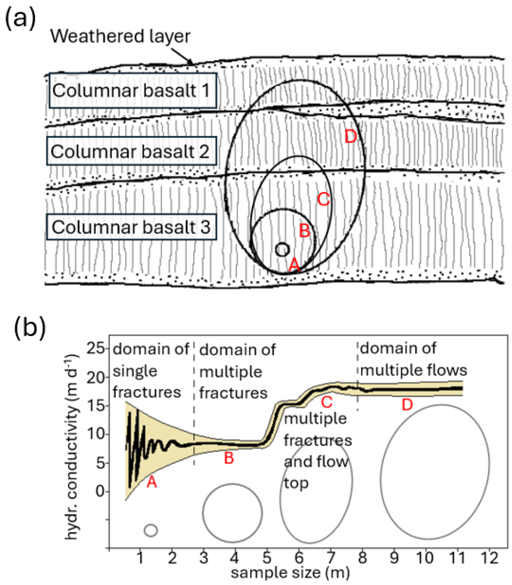
1. Introduction
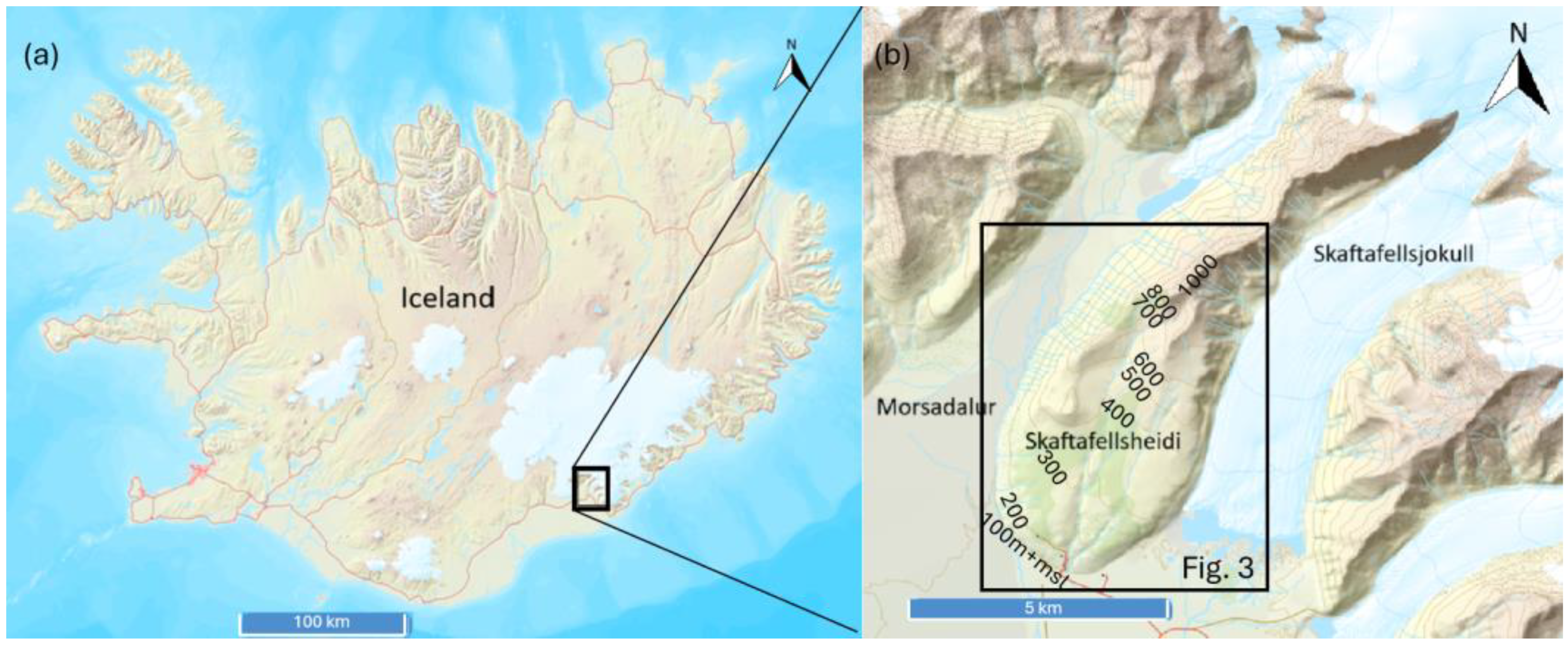
2. Materials and Methods
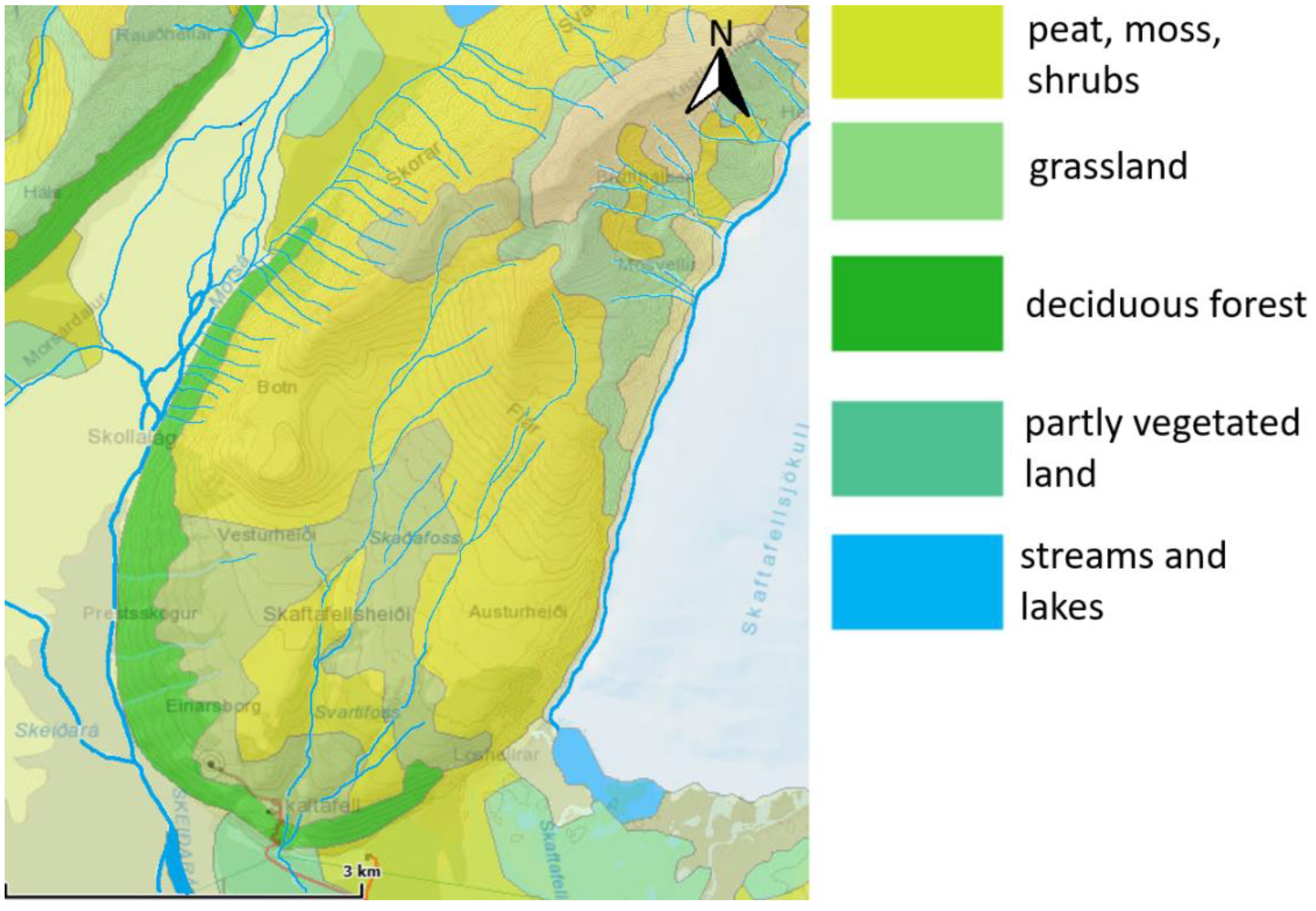
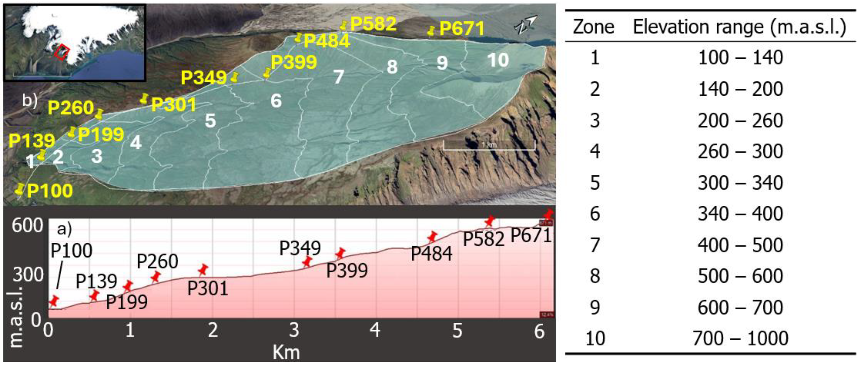
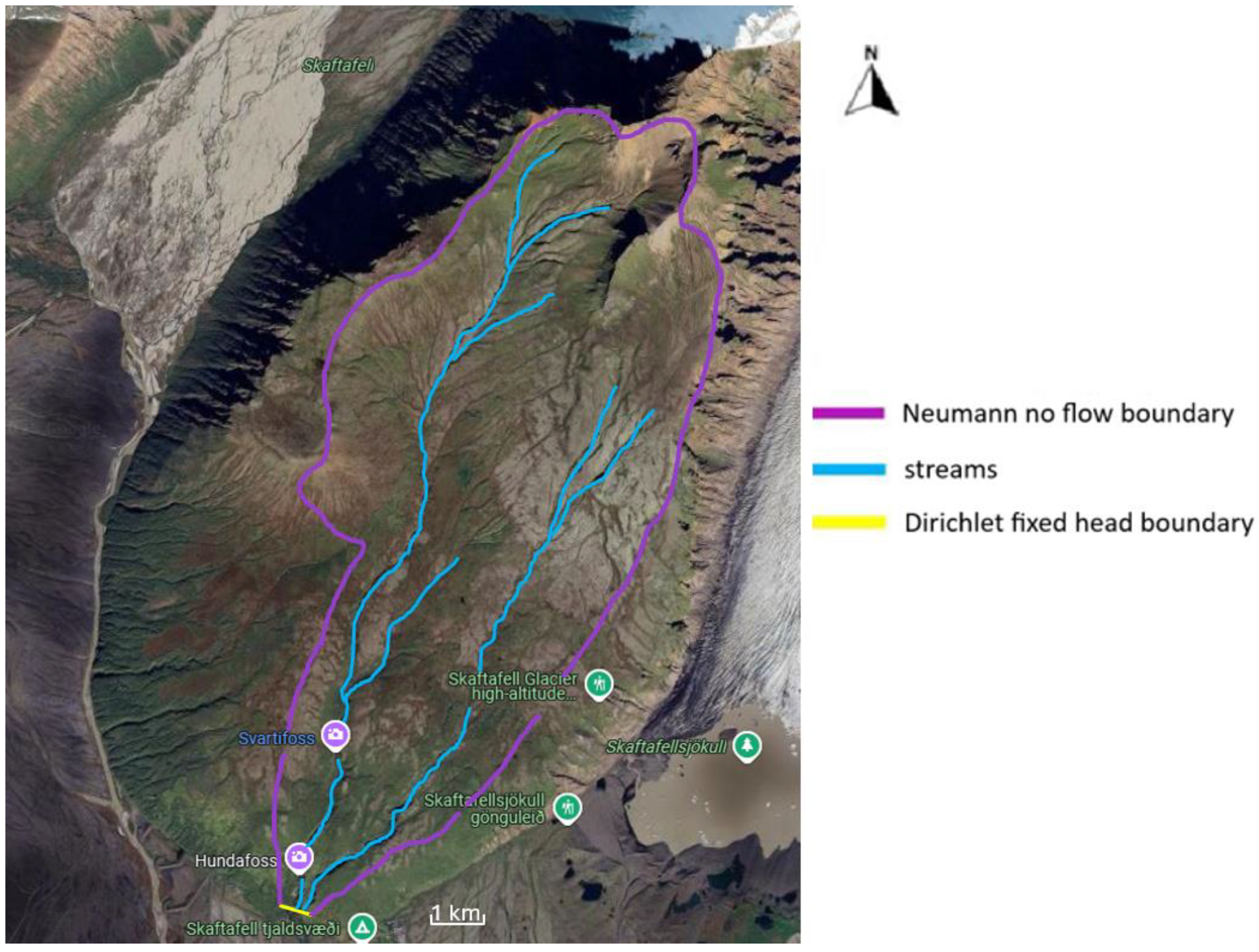
2.1. Field Campaign Setup
Water Balance
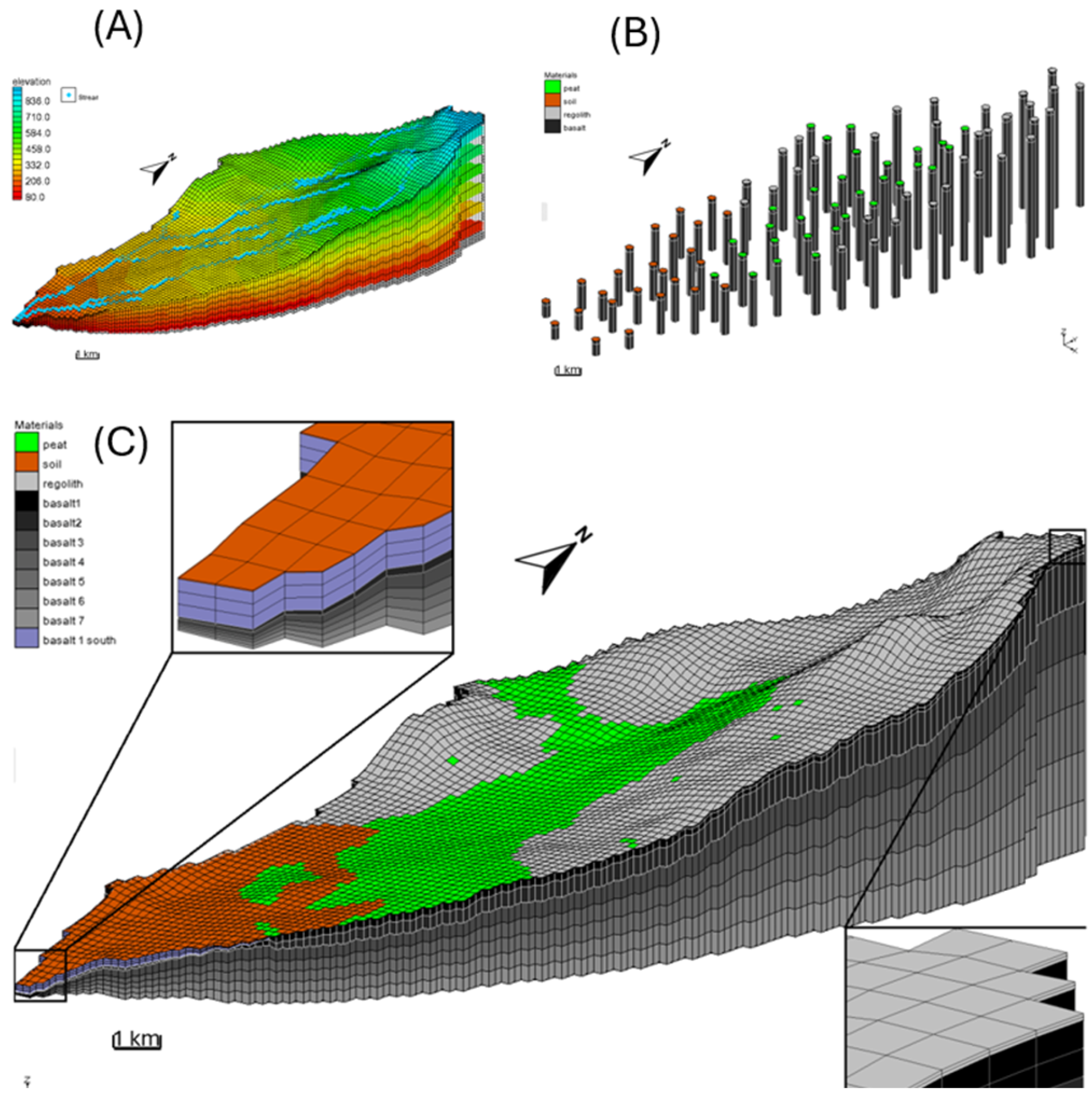
2.2. Model Setup
3. Results
3.1. Field Campaign Results
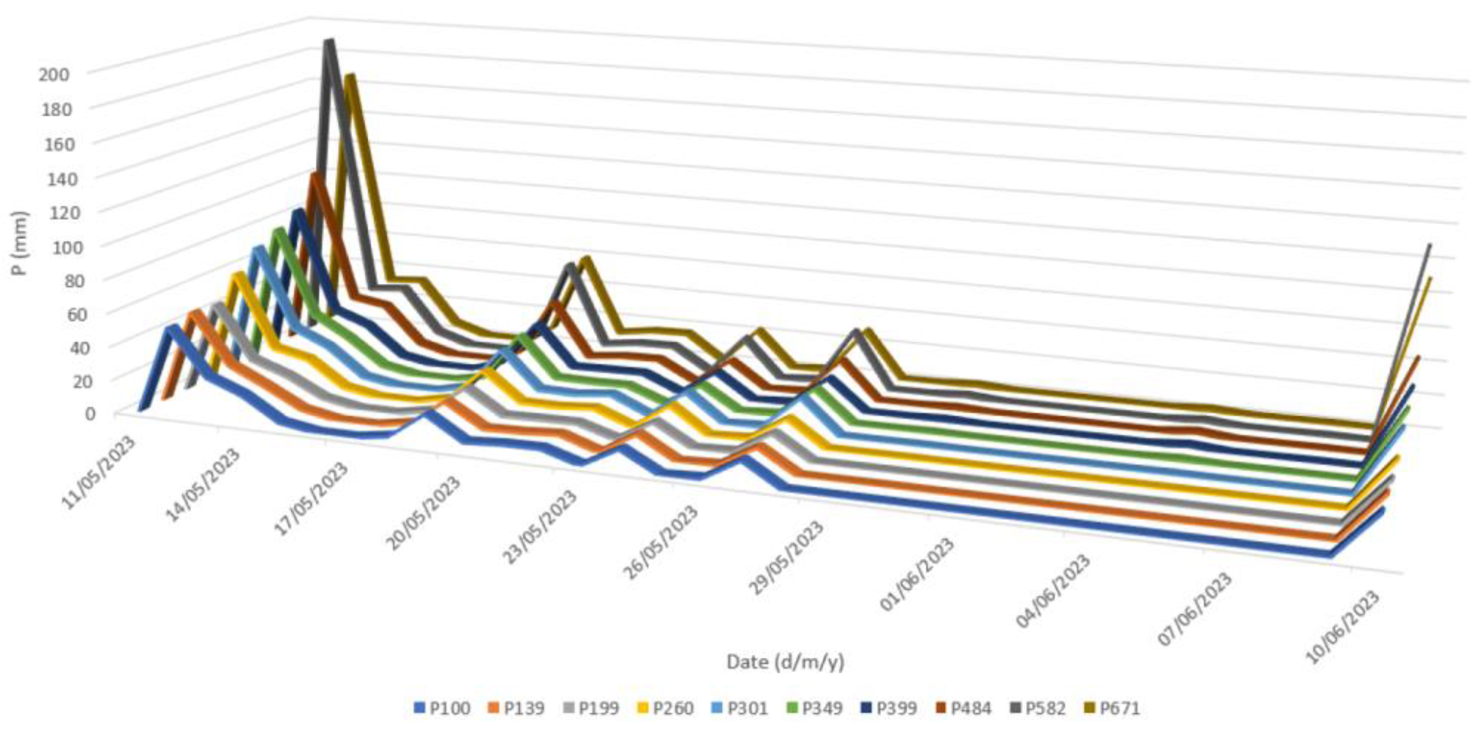
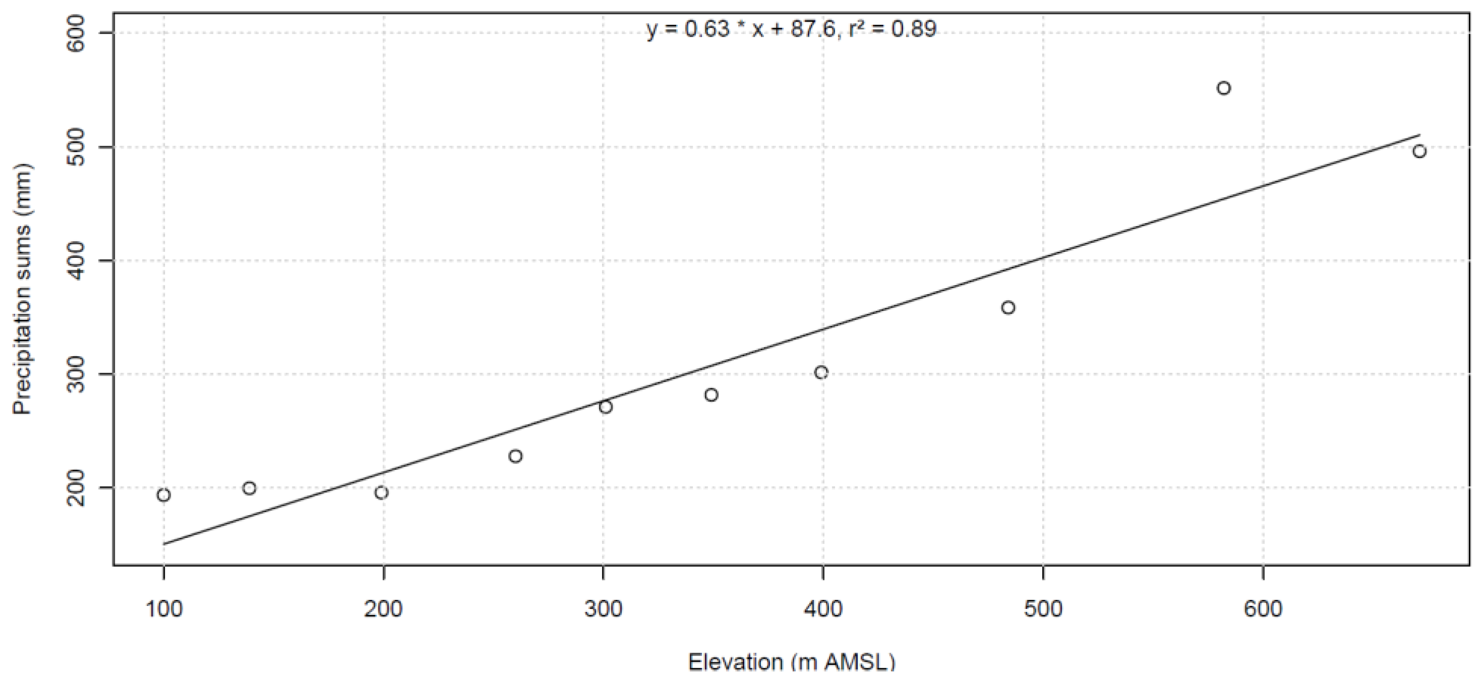
3.1.1. Precipitation
3.1.2. Snowmelt
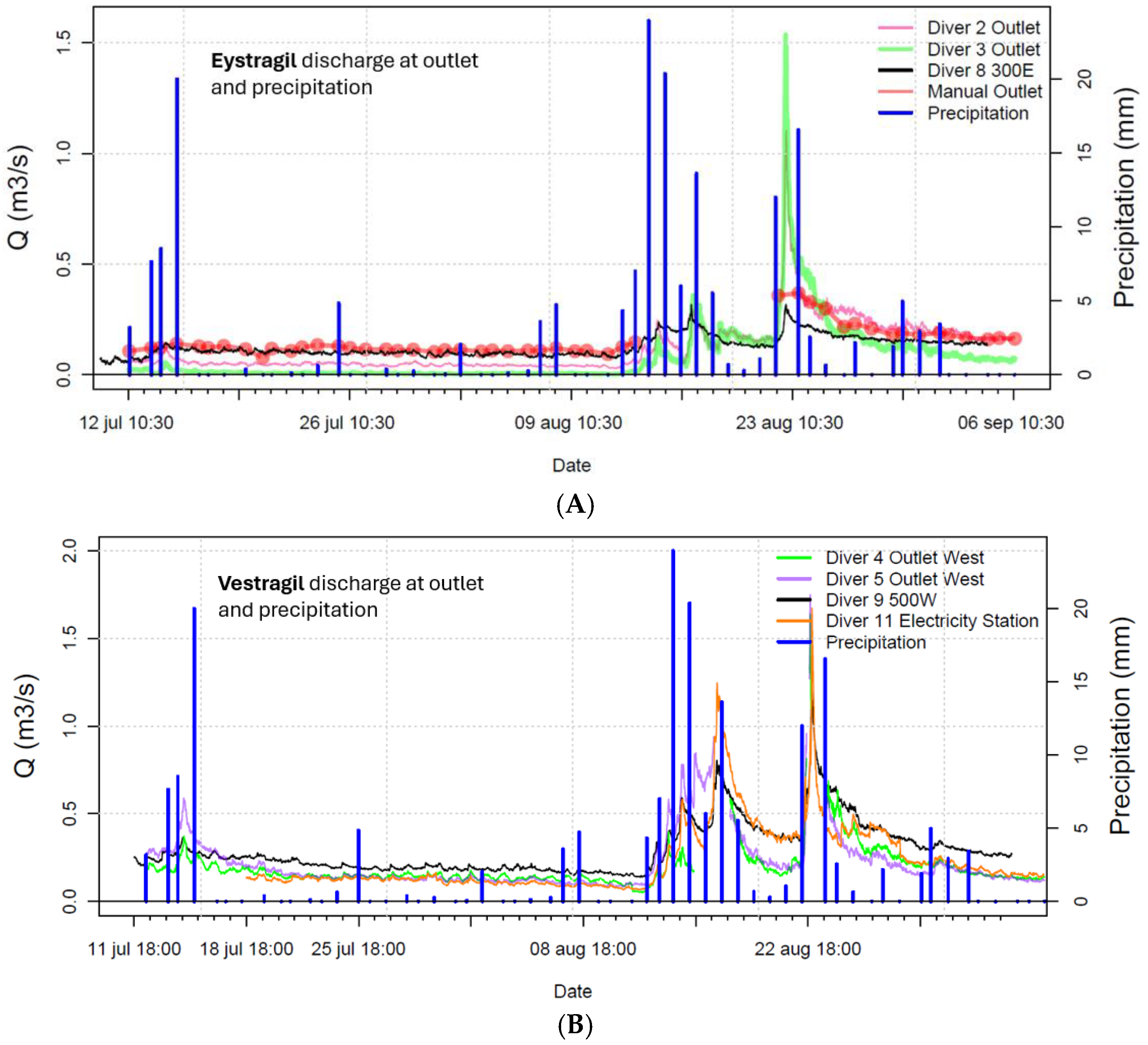
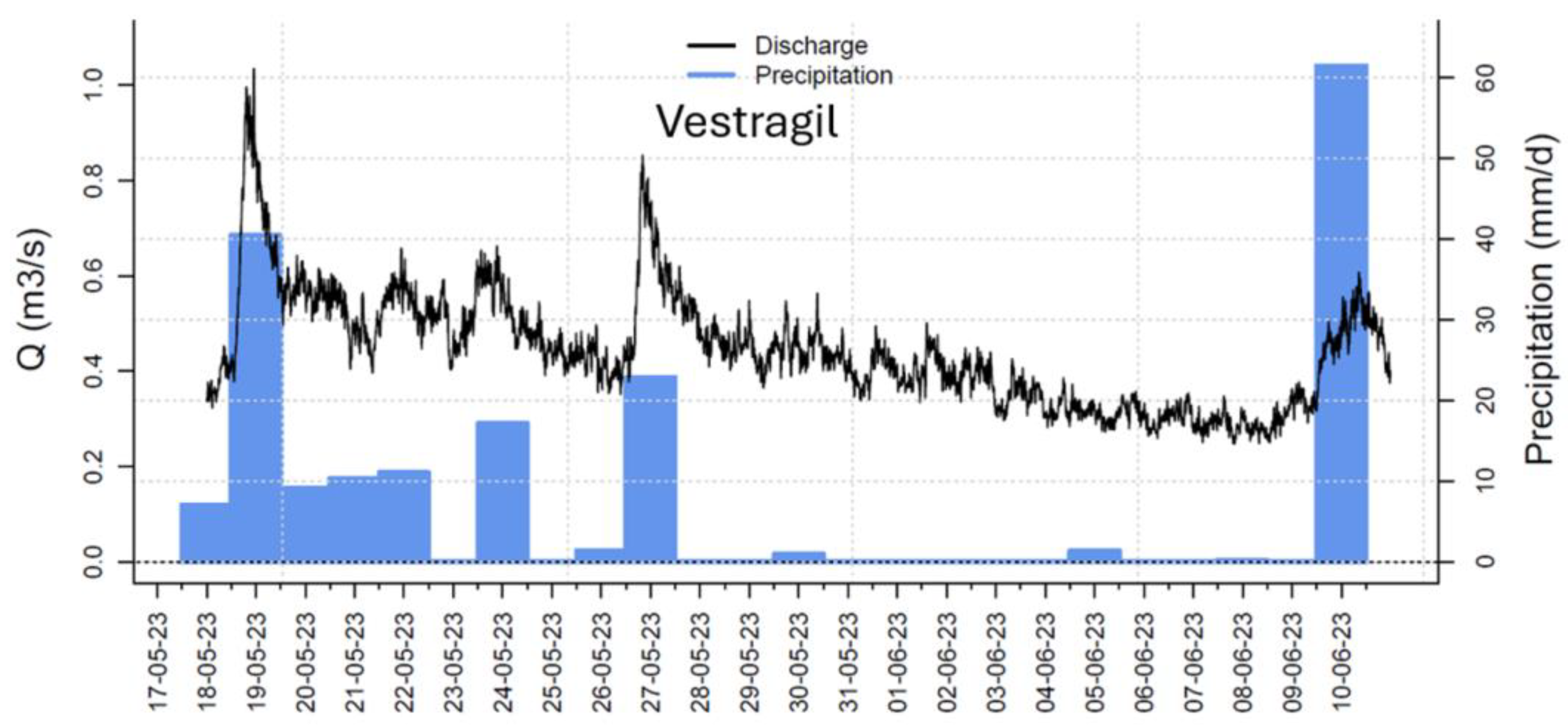
3.1.3. Discharge
3.1.4. Evapotranspiration
3.1.5. Water Balance
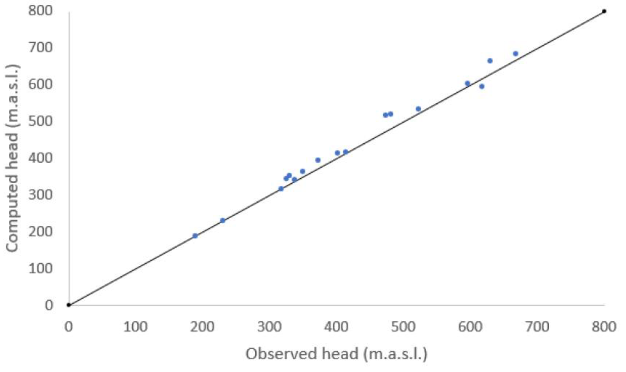
3.2. Modeling Results
4. Discussion
5. Conclusions
Author Contributions
Funding
Data Availability Statement
Acknowledgments
Conflicts of Interest
Abbreviations
| REV | Representative elementary volume |
References
- Dijksma, R.; Brooks, E.S.; Boll, J. Groundwater recharge in Pleistocene sediments overlying basalt aquifers in the Palouse Basin, USA: Modeling of distributed recharge potential and identification of water pathways. Hydrogeol. J. 2011, 19, 489–500. [Google Scholar] [CrossRef]
- Versey, H.R.; Singh, B.K. Groundwater in Deccan basalts of the Betwa Basin, India. J. Hydrol. 1982, 58, 279–306. [Google Scholar] [CrossRef]
- Candel, J.; Brooks, E.S.; Sanchez-Murillo, R.; Grader, G.; Dijksma, R. Identifying recharge connections in the Moscow (USA) sub-basin using tracers and a soil moisture routing model. Hydrogeol. J. 2016, 24, 1739–1751. [Google Scholar] [CrossRef]
- Brown, K.B.; McIntosh, J.C.; Rademacher, L.K.; Lohse, K.A. Impacts of agricultural irrigation recharge on groundwater quality in a basalt aquifer system (Washington, USA): A multi-tracer approach. Hydrogeol. J. 2011, 19, 1039–1051. [Google Scholar] [CrossRef]
- Taylor, R.G.; Howard, K.W.F. The dynamics of groundwater flow in the regolith of Uganda. Int. Contrib. Hydrogeol. 1998, 18, 97–114. [Google Scholar]
- Gropius, M.; Dahabiyeh, M.; Al Hyari, M.; Brückner, F.; Lindenmaier, F.; Vassolo, S. Estimation of unrecorded groundwater abstractions in Jordan through regional groundwater modelling. Hydrogeol. J. 2022, 30, 1769–1787. [Google Scholar] [CrossRef]
- Hancox, J.; Gárfias, J.; Aravena, R.; Rudolph, D. Assissing the vulnerability of over-exploited volcanic aquifer systems using multi-parameter analysis, Tucola Basin, Mexico. Environ. Earth Sci. 2010, 59, 1643–1660. [Google Scholar] [CrossRef]
- Liu, H.H.; Doughty, C.; Boðvarsson, G.S. An active fracture model for unsaturated flow and transport in fractured rocks. Water Resour. Res. 1998, 34, 2633–2646. [Google Scholar] [CrossRef]
- MacDonald, D.M.J.; Kulkami, H.C.; Lawrence, A.R.; Deolankar, S.B.; Barker, J.A.; Lalwani, A.B. Sustainable groundwater development of hard-rock aquifers: The conflict between irrigation and drinking water supplies from the Deccan basalts of India. In British Geological Survey NERC Technical Report WC/95/52; 1995; 54p. [Google Scholar]
- Domenico, P.A.; Schwartz, F.W. Physical and Chemical Hydrogeology, 2nd ed.; John Wiley and Sons: Hoboken, NJ, USA, 1997; ISBN 978-0-471-59762-9. [Google Scholar]
- Dijksma, R.; Avis, L. Measuring and modelling water transport on Skaftafellsheiði, Iceland. Forum Geogr. 2016, XV, 66–72. [Google Scholar] [CrossRef]
- Pyatt, F.B.; Ditcham, D. A contribution to the study of the ecology of Iceland: The ecology of a scree slope on Skaftafellsheiði and a Sandur area. Int. J. Environ. Stud. 1983, 20, 299–306. [Google Scholar] [CrossRef]
- Grunngerð Landupplýsingátt. Available online: https://kort.gis.is/mapview/ (accessed on 25 February 2025).
- Guðmundsson, A.T. Living Earth: Outline of the Geology of Iceland; Mal og Menning: Reykjavik, Iceland, 2007; ISBN 978-9979-3-3360-9. [Google Scholar]
- Helgason, J.; Duncan, R.A. Glacial-interglacial history of the Skaftafell region, southeast Iceland, 0–5 MA. Geology 2001, 29, 179–182. [Google Scholar] [CrossRef]
- Wood, W.W.; Fernandez, L.A.; Back, W.; Rosenshein, J.S.; Seaber, P.R. Volcanic rocks. Hydrogeology 1988, 2, 353–365. [Google Scholar]
- Helgason, J. Bedrock Geological Map of Skaftafell, SE-Iceland; Geological Consulting: Reykjavik, Iceland, 2007. [Google Scholar]
- Hiscock, K.M.; Bense, V.F. Hydrogeology: Principles and Practice; John Wiley and Sons: Hoboken, NJ, USA, 2014. [Google Scholar]
- Singal, B.B.S.; Gupta, R.P. Applied Hydrogeology of Fractured Rocks; Springer Science and Business Media: Berlin/Heidelberg, Germany, 2010. [Google Scholar]
- Wellman, T.P.; Poeter, E.P. Estimating spatially variable representative elementary scales in fractured architecture using hydraulic head observations. Water Resour. Res. 2005, 41. [Google Scholar] [CrossRef]
- Avis, L. Estimating Hydrological Characteristics of a Basaltic Catchment Using Simple Field Measurements and Modelling; a Case Study in Skaftafell National Park, Iceland. Master’s Thesis, Wageningen University, Wageningen, The Netherlands, 2016. [Google Scholar]
- Beck, H.E.; Zimmermann, N.; McVicar, T.R.; Vergopolan, N.; Berg, A.; Woord, E.F. Present and future Köppen-Geiger climate classification maps at 1-km resolution. Sci. Data 2018, 5, 180214. [Google Scholar] [CrossRef]
- Available online: https://vedur.is/ (accessed on 15 April 2025).
- Spreen, W.C. A determination of the effect of topography upon precipitation. EOS Trans. Am. Geophys. Union 1947, 28, 285–290. [Google Scholar]
- Winkler, M.; Schellander, H.; Gruber, S. Snow water equivalents exclusively from snow depths and their temporal changes: The Δsnow. EGU Hydrol. Earth Syst. Sci. 2021, 25, 1165–1187. [Google Scholar] [CrossRef]
- Hargreaves, G.H.; Samani, Z.A. Estimating potential evapotranspiration. J. Irrig. Drain. Div. 1982, 108, 225–230. [Google Scholar] [CrossRef]
- Samani, Z. Estimating solar radiation and evapotranspiration using minimum climatological data. J. Irrig. Drain. Eng. 2000, 126, 265–267. [Google Scholar] [CrossRef]
- Valiantzas, J.D. Simplified versions for the Penman evaporation equation using routine weather data. J. Hydrol. 2006, 331, 690–702. [Google Scholar] [CrossRef]
- Zweers, E.A. Hydrological Boundaries of a Basaltic Catchment: In Situ Measurements and Modelling of the Basalt Outcrop in Skaftafellsheiði, Iceland. Master’s Thesis, Wageningen University, Wageningen, The Netherlands, 2023. [Google Scholar]
- Harbaugh, A.W. MODFLOW-2005, the U.S. Geological Survey modular groundwater model. In US Geological Survey Techniques and Methods; 2005; Volume 6-A16. [Google Scholar]
- McDonald, M.G.; Harbaugh, A.W. A Modular Three-Dimensional Finite-Difference Groundwater Flow Model; US Geological Survey: Reston, VA, USA, 1988. [Google Scholar]
- Doherty, J. Calibration and uncertainty analysis for complex environmental models. Watermark Numer. Comput. Brisb. Aust. 2015, 227. [Google Scholar]
- Khaleel, R. Scale dependence of continuum models for fractured basalts. Water Resour. Res. 1989, 25, 1847–1855. [Google Scholar] [CrossRef]
- Magnuson, S.O. Inverse modeling for Field-Scale Hydrologic and Transport Parameters of Fractured Basalt; Lockheed Idaho Technologies CO: Idaho Falls, ID, USA, 1995; INEL-95/0637. [Google Scholar]
- Fetter, C.W.; Kreamer, D. Applied Hydrogeology, 5th ed.; Waveland Press Inc.: Long Grove, IL, USA, 2022; ISBN 978-1-4786-4652-5. [Google Scholar]
- Kooi, M. Hydrological Responses in a Basaltic Catchment: A Case Study on Iceland. Master’s Thesis, Wageningen University, Wageningen, The Netherlands, 2015. [Google Scholar]
- Brooks, E.S.; Boll, J.; McDaniel, P.A. A hillslope-scale experiment to measure lateral saturated hydraulic conductivity. Water Resour. Res. 2004, 40. [Google Scholar] [CrossRef]
- Hannesdóttir, H.; Aðalgeirsdóttir, G.; Jóhannesson, T.; Guðmundsson, S.; Crochet, P.; Ágústsson, H.; Pálsson, F.; Magnússon, E.; Sigurðsson, S.Ð.; Björnsson, H. Downscaled precipitation applied in modelling of mass balance and the evolution of souteast Vatnajökull, Iceland. J. Glaciol. 2025, 61, 799–813. [Google Scholar] [CrossRef]
- Einarsson, M.A. Potential evapotranspiration and water balance in Iceland. Hydrol. Res. 1972, 3, 183–198. [Google Scholar] [CrossRef]
- Einarsson, M.A. Climate of Iceland. Elsevier World Surv. Climatol. 1984, 15, 673–697. [Google Scholar]
- Verma, K.; Katpatal, Y. Groundwater monitoring using GRACE and GLDAS data after downscaling within basaltic aquifer system. Groundwater 2020, 58, 143–151. [Google Scholar] [CrossRef]


| January | February | March | April | May | June | July | August | September | October | November | December | Avg | |
|---|---|---|---|---|---|---|---|---|---|---|---|---|---|
| P | 145 | 130 | 130 | 115 | 118 | 131 | 121 | 159 | 141 | 185 | 137 | 133 | 137 |
| T | −0.4 | 0.2 | 0.7 | 3.2 | 6.5 | 9.4 | 11.2 | 10.4 | 7.5 | 4.5 | 1.1 | −0.4 | 4.5 |
| Zone | Vegetation Type | Elevation Range (m + msl) | Kc | fc |
|---|---|---|---|---|
| 1 | Deciduous forest | 100–200 | 0.9 | 0.9 |
| 2 | Peat (willows) | 200–300 | 0.9 | 0.8 |
| 3 | Peat (bog, forest, grass) | 300–400 | 0.9 | 1 |
| 4 | Moss | 400–540 | 0.15 | 0.6 |
| 5 | Vegetated regolith | 540–700 | 0.45 | 0.45 |
| 6 | Bare regolith | 700–1000 | 0.2 | 0 |
| Material | Thickness (m) | kh (m d−1) | kv (m d−1) | Specific Storage (m−1) | Specific Yield (−) |
|---|---|---|---|---|---|
| organic soil | 0.5 | 5 | 5 | 1 × 10⁻⁶ | 0.08 |
| peat | 2–4 | 5 | 5 | 1 × 10⁻⁶ | 0.2 |
| regolith | 2 | 10 | 10 | 1 × 10⁻⁶ | 0.4 |
| basalt 1 | 10 | 0.3 | 10 | 1 × 10⁻⁶ | 0.4 |
| basalt 2 | 1–134 | 0.3 | 0.3 | 1 × 10⁻⁶ | 0.4 |
| basalt 3–7 | 1–134 | 0.01 | 0.01 | 1 × 10⁻⁶ | 0.4 |
| Water Balance | P | M | Q | ETpot | ΔS |
|---|---|---|---|---|---|
| July/August 2015 | |||||
| 106 m3 | 2.05 | 0.24 | 1.49 | 0.66 | 0.14 |
| mm | 206 | 25 | 150 | 67 | 14 |
| May/June 2023 | |||||
| 106 m3 | 1.9 | 0.16 | 3.0 | 0.50 | 1.44 |
| mm | 190 | 17 | 300 | 51 | 144 |
Disclaimer/Publisher’s Note: The statements, opinions and data contained in all publications are solely those of the individual author(s) and contributor(s) and not of MDPI and/or the editor(s). MDPI and/or the editor(s) disclaim responsibility for any injury to people or property resulting from any ideas, methods, instructions or products referred to in the content. |
© 2025 by the authors. Licensee MDPI, Basel, Switzerland. This article is an open access article distributed under the terms and conditions of the Creative Commons Attribution (CC BY) license (https://creativecommons.org/licenses/by/4.0/).
Share and Cite
Dijksma, R.; Bense, V.; Zweers, E.; Avis, L.; van der Ploeg, M. Hydrological Characteristics of Columnar Basalt Aquifers: Measuring and Modeling Skaftafellsheiði, Iceland. Geosciences 2025, 15, 160. https://doi.org/10.3390/geosciences15050160
Dijksma R, Bense V, Zweers E, Avis L, van der Ploeg M. Hydrological Characteristics of Columnar Basalt Aquifers: Measuring and Modeling Skaftafellsheiði, Iceland. Geosciences. 2025; 15(5):160. https://doi.org/10.3390/geosciences15050160
Chicago/Turabian StyleDijksma, Roel, Victor Bense, Eline Zweers, Lisette Avis, and Martine van der Ploeg. 2025. "Hydrological Characteristics of Columnar Basalt Aquifers: Measuring and Modeling Skaftafellsheiði, Iceland" Geosciences 15, no. 5: 160. https://doi.org/10.3390/geosciences15050160
APA StyleDijksma, R., Bense, V., Zweers, E., Avis, L., & van der Ploeg, M. (2025). Hydrological Characteristics of Columnar Basalt Aquifers: Measuring and Modeling Skaftafellsheiði, Iceland. Geosciences, 15(5), 160. https://doi.org/10.3390/geosciences15050160