Abstract
Approximately 70% of global tsunamis are generated within the pan Pacific Ocean region. This paper reports on detailed analysis of civilian video footage from the 2011 Tohoku earthquake, Japan. Comprehensive scientific analysis of tsunami video footage can yield valuable insights into geophysical processes and impacts. Civili22an video footage captured during the 2011 Tohoku, East Honshu, Japan tsunami was critically examined to identify key tsunami processes and estimate local inundation heights and flow velocity in Kesennuma City. Significant tsunami processes within the video were captured and orientated in ArcGIS Pro to create an OIC (Oriented Imagery Catalogue). The OIC was published to ArcGIS Online, and the oriented imagery was configured into an interactive website. Flow velocity was estimated by quantifying the distance and time taken for an object to travel between two known points in the video. Estimating inundation height was achieved by taking objects with known or calculable dimensions and measuring them against maximum local inundation height observations. The oriented imagery process produced an interactive Experience Builder app in ArcGIS Online, highlighting key tsunami processes captured within the video. The estimations of flow velocity and local inundation height quantified during video analysis indicate flow speeds ranging from 2.5–4.29 m/s and an estimated maximum local run-up height of 7.85 m in Kesennuma City. The analysis of civilian video footage provides a remarkable opportunity to investigate tsunami impact in localised areas of Japan and around the world. These data and analyses inform tsunami hazard maps, particularly in reasonably well-mapped terrains with remote access to landscape data. The results can aid in the understanding of tsunami behaviours and help inform effective mitigation strategies in tsunami-vulnerable areas. The affordable, widely accessible analysis and methodology presented here has numerous applications, and does not require highly sophisticated equipment. Tsunamis are a significant to major geohazard globally including many Pacific Island states, e.g., Papua New Guinea, Solomon Islands, and Tonga. Video footage geoscientific analysis, as here reported, can benefit tsunami and cyclone storm surge hazards in the Pacific Islands region and elsewhere.
1. Introduction
1.1. Tsunamis
Tsunamis are a significant geohazard for Pacific Island states, including Papua New Guinea, Solomon Islands, and Tonga. Hagen et al. [1] reported on the impacts of the large 2007 tsunami in the western Solomon Islands area. Although this paper is a case study from eastern Honshu, Japan, the method and approach reported in this paper can be used for geohazard assessments within the Pacific Islands region, and globally, as increasing proportions of their populations have access to smartphones and, through this, portable video-making technologies. This paper is part of a volume that will be read widely by people in Papua New Guinea and the Pacific Islands region, and the authors want to emphasise the relevance of this study to their tsunami prone region and all tsunami-prone regions.
The term tsunami originates from the Japanese language, meaning harbour (“tsu”) and wave (“nami”) [2]. Tsunamis are ocean waves; however, they vary greatly from ‘normal’ waves usually seen in the ocean, due to their distinctive mode of generation, wavelength, and velocity [2]. The generation of most tsunamis can be attributed to disturbances producing seismic motions under the sea; these disturbances include submarine earthquakes, landslides, and volcanic eruptions [3]. Studies on confirmed tsunami generation mechanisms have shown that 80% of tsunamis are generated by earthquakes, with the other 20% caused by earthquake-generated landslides, volcanic eruptions, other landslides, and other sources [4]. Figure 1 shows the distribution of tsunami sources from 1610 B.C to A.D 2018, with most of these represented by red circles, indicating earthquakes as the predominant tsunami generation mechanism.
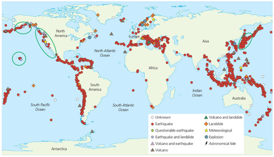
Figure 1.
World map of historical tsunami sources, dating from 1610 B.C to A.D 2018. Sources of tsunami: open white circle (unknown); red circle (earthquake); green circle (questionable); blue circle (earthquake + landslide); light grey triangle (volcano + earthquake); dark grey triangle (volcano); green triangle (volcano + landslide); brown cross (landslide); star (meteorological); blue circle with cross (explosion); lighting symbol (astronomical). Green ovals indicate areas of particularly high tsunami risk. Acknowledgement: NOAA, 2013 [4]. Note that most of these tsunamis were generated by earthquake, particularly at subduction zones, and note their abundant distribution along the Pan-Pacific subduction zone. Circles represent earthquake-generated tsunamis, triangles represent volcanic-generated tsunamis, and squares represent landslide-generated tsunamis.
The distribution of tsunami sources shows a clear pattern of predominant generation within tectonic subduction zones, most of these being along the Pan-Pacific subduction zone (Figure 1). Overall, 69% of tsunami sources are found within the Pacific Ocean, followed by 17% in the Mediterranean Sea, 9% in the Caribbean Sea and Atlantic Ocean, and 5% in the Indian Ocean [3,4].
1.2. Tsunami Generation and Transport through the Ocean
Subduction zones are found at convergent tectonic plate boundaries, where one plate subducts beneath another into the underlying mantle [3]. Stress produced through plate convergence can build up for decades/centuries, until the stress exceeds the local rock strength and energy is released in the form of an earthquake [3]. Subduction zones produce some of the strongest earthquakes in the world, termed megathrust earthquakes, indicating large thrust faults as their primary mode of genesis. When these earthquakes occur under the ocean, they are capable of producing tsunami waves tens of metres high [3]. Tsunamis produced through undersea earthquakes have three main stages: (1) tsunami generation, (2) mid-ocean propagation, and (3) coastal propagation and inundation [2]. The first stage is tsunami generation, the initial formation of the tsunami e.g., through the tectonic rise or fall in sea level (Figure 2) [2]. The majority of tsunamigenic undersea earthquakes occur at subduction zones through strike-slip, thrust, or normal faulting [2]. Converging tectonic plates at subduction zones build up stress along these fault lines when there is an obstruction to their motion [3]. The stress is then released by the sudden movement of the overriding plate springing upwards, resulting in the vertical upward–downward displacement of the seafloor (Figure 2) [3]. This displacement of the Earth’s crust also greatly disturbs the overlying water column, forcing it upwards, forming tsunami waves [3].
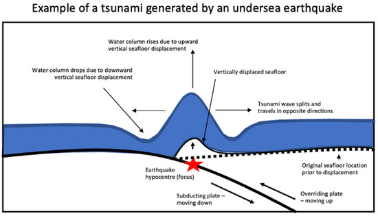
Figure 2.
Stage 1: tsunami generation, the formation of a tsunami through an undersea earthquake. The vertical displacement of the sea floor disturbs the overlying water column, creating the tsunami wave (diagram adapted from [2], 2008, drafted and designed by McDonough-Margison).
The second stage is mid-ocean propagation. Tsunami waves travel at great speeds through the ocean with little energy loss due their very large wavelength [2]. The depth of the water directly correlates to the speed of the tsunami, the deeper the water, the faster the wave travels. For example, if the ocean water depth is 6100 m, the wave can reach speeds of 890 km/h (Figure 3) [2]. As the tsunami reaches the coast, the water depth decreases, which, in turn, decreases the wave velocity [2].
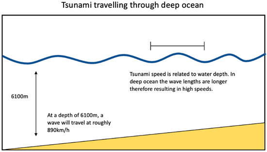
Figure 3.
This diagram explains stage 2: the movement of a tsunami wave during deep ocean propagation. Here, the tsunami wave travels at high speeds through the deep ocean (diagram drafted using information provided by [2], drafted and designed by McDonough-Margison).
The final stage is coastal propagation and inundation. When a tsunami is travelling through the deep ocean it may appear harmless; however, as it reaches the coastline, it can produce a wave tens of metres high. As the tsunami approaches the coast, the ocean depth decreases, causing the wavelength to also decrease, whilst total tsunami energy remains the same [2], (Figure 4). The wave is forced into a smaller area and compressed as it reaches the shore, resulting in increased wave amplitude (height) [5]; this effect is known as shoaling. This situation can produce an onshore wave run-up height upwards of 40 m in some cases [3] (Figure 4). Terms such as tsunami run-up and inundation/inundation height are frequently used with respect to tsunami phenomena, but can cause a degree of confusion in their definition. For this paper, we are using the definitions of ‘a peak in tsunami wave relative to mean sea level, measured in vertical height of maximum tsunami wave height relative to mean sea level’ for tsunami run-up, and ‘the maximum horizontal distance a tsunami travels inland from the coastline’ for inundation, with ‘local run-up height or local inundation maximum height’ as terms that specify the maximum local elevation within an inland location of the tsunami.
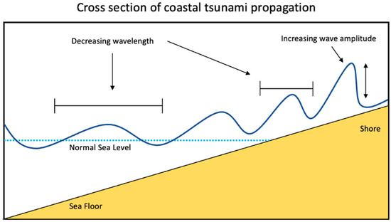
Figure 4.
Diagram showing stage 3: coastal tsunami propagation and inundation. The wavelength is decreasing and the wave amplitude is increasing as it reaches the shore (diagram adapted from [2], drafted and designed by McDonough-Margison).
1.3. Regional Setting of Japan
Overall, 69% of the worlds confirmed tsunami sources are located within the Pacific Ocean. Of these, 20% are located within Japanese waters [4], which can be attributed to Japan’s extremely active geological setting along the Pan-Pacific Subduction Zone [6]. The high geological activity of the Japanese arc is caused by the interaction between five plates: the Eurasian, Amur, Okhotsk, Pacific, and Philippine plates [6]. This region experiences 1/10 of the worlds earthquakes [7], with seismicity in this area being linked to the interactions of these plates/plate boundaries and active fault systems [8]. Between 1976 and 2012, 76.3% of these earthquakes in the Japan arc occurred offshore, posing potential tsunami risks [6]. The earthquake and tsunami interoccurrence times in Japan are 186.23 days and 273.31 days, respectively, making this one of the most tsunamically active regions in the world [6].
Earthquakes of various depths and types occur along the Japanese arc [7]. Much of this seismic activity is concentrated on the Pacific side of the country, along the Japan trench plate boundary between the Pacific and Okhotsk plates (Figure 5). At this plate boundary, shallow thrust-forming and tsunamigenic subduction generated megathrust earthquakes occur [7,9]. The Japan trench plate boundary is the most active earthquake-generating location within the Japanese arc, with more than 100 earthquakes over M6 (magnitude 6) since 1885 [8]. The high earthquake activity is due to the geological structure and convergence rate at the trench plate boundary [9]. Due to its offshore location, the Japan trench is responsible for generating tsunamis through these subduction zone quakes [8]. The Nankai trough, located in the south-east of Japan, where the Philippine Sea and Amur Plates collide, is also an area of significant seismicity. This area produces an earthquake larger than M8 at intervals of roughly 180 years and, historically, has produced large, devastating tsunamis [8,10,11]. While much of Japan’s seismicity is concentrated on the Pacific side of the country, the western side of Japan is also known to experience active seismicity in the Japan sea margin [12]. However, with an absence of megathrust subduction earthquakes, less frequent events, and lower seismicity, this area experiences fewer tsunamigenic earthquakes in comparison to the Pacific Coast [9,13].
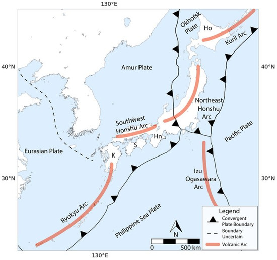
Figure 5.
Tectonic map of the Japan region showing the positions of the Pacific, Philippine Sea, Eurasian, Amur, and Okhotsk Plate [8], acknowledgements to Creative Commons for permission to reproduce.
Japan faces the greatest risk of tsunamis compared to anywhere else in the world, due to its proximity to an active subduction zone and its high population concentration along the coastline adjacent to this zone [14]. Japan’s extreme vulnerability to tsunami events was witnessed during the 2011 Tohuku earthquake and tsunami.
1.4. The 2011 Tohuku Earthquake and Tsunami
On 11 March 2011, at 14:46 (JST), a magnitude 9.0 earthquake struck off the coast Japan’s largest island, Honshu [15]. The earthquake had an estimated location of 38.322° N and 142.369° E, only 129 km from Sendai, and a depth of 32 km (Figure 6) [15]. The fault rupture occurred along the subduction zone where the Pacific plate dives beneath Japan, parallel to the Japan trench [16]. The entirety of the megathrust fault located in the Tokuku-oki region failed during this event; both up-dip (up-slope) and down-dip (down-slope) motions occurred [17]. A fault failure this significant was not previously anticipated in hazard models [17].
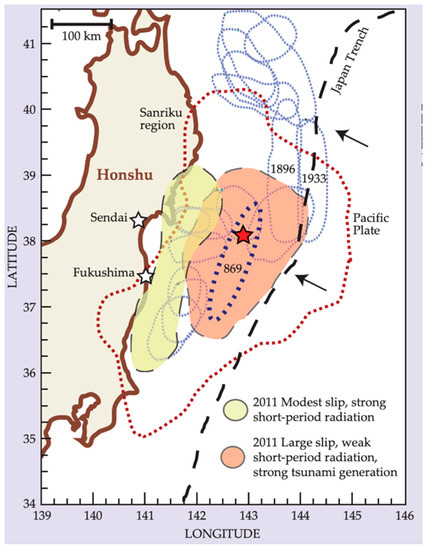
Figure 6.
Map showing the fault ruptures during the 2011 Tohuku earthquake. The light green colour shows moderate slips, whereas the light red colour shows the fault slip areas where tsunami generation was possible. Within this red area is the epicentre of the earthquake (red star) and a blue dotted oval showing the 898 earthquakes, the only other known event with the same megathrust rupture zone. The dotted red line shows the aftershocks 24 h after the main earthquake, and the smaller blue lines indicate the location of significant past earthquake events (acknowledgement to [17]).
The fault rupture began off the coast of the Miyagi Prefecture and propagated both north in the direction of the Iwate Prefecture and south in the direction of the Fukushima prefecture [18]. The earthquake lasted for roughly 150 s; the first 50 s of the fault rupture experienced relatively low expansion, at a rate of 1 km/s [17,18]. Over the next 40 s, the rupture expanded to shallower depths, where the largest slip occurred close to the trench. This slip was 40 m over the upper 100 km of the megathrust fault, with 60–80 m slips measured locally [17]. This was an unusually large slip in such a localised area and the largest documented fault displacement in history [17]. Sliding further down, the slope (down-dip) progressed southward parallel to the coastline at a rate of roughly 2.5 km/s [17]. The total rupture area is indicated in (Figure 6) by the light green and light red areas of the map.
The deformation caused by this rupture moved the Japan coast up to 5 m eastward and vertically displaced the ocean floor as much as 5 m over an area of roughly 15,000 km2 [17]. This displacement produced a catastrophic tsunami reaching run up heights of 40 m in areas situated along the east coast (Figure 7). Figure 7 shows the run-up and inundation heights of the tsunami on the east coast of Japan, with the wave in most of the areas exceeding the height of the Fukushima power plant tsunami wall, also indicated on the diagram.
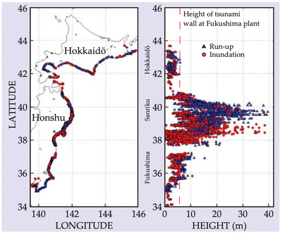
Figure 7.
Diagram showing the tsunami inundation and run-up heights along the east coast of Japan. Areas in Sanriku had inundation and run-up heights just shy of 40 m ([17] acknowledged).
The consequences of this event were highly impactful, with nearly 20,000 lives lost. East coast regions were the most affected, with the prefectures of Iwate, Miyagi, and Fukushima making up 99% of the total deaths as a result of this event [19]. Most of the casualties were not caused by earthquake itself, but by the tsunami, which overtopped coastal tsunami break walls and completely inundated towns [19]. Along with loss of life, there were several other social, economic, and environmental impacts. Key impacts include [15] 190,000 buildings damaged, including 45,700 completely destroyed; an estimated 23,600 ha of farmland destroyed; impacts to transport- e.g., 62 of 70 railway lines affected; adverse impacts to manufacturers including Toyota, Nissan, Honda, and Mitsubishi; estimated direct economic loss of about 171–183 billion USD; further impacts to both the mental and physical health of those affected; and the infamous Fukushima Nuclear Powerplant disaster.
1.5. Kesennuma City Case Study
Kesennuma City, located in the northeast of the Miyagi prefecture in eastern Japan, was one of the more impacted areas during the 2011 Tokuku earthquake and tsunami (Figure 8). Kesennuma is one of Japan’s most tsunami-vulnerable cities, having been affected by a number of previous tsunamis, including 1896 Meiji-Sanriku, 1933 Showa-Sanriku, and the 1960 and 2010 Chilean tsunamis [20,21,22]. Evacuations are held annually in Kesennuma to prepare for such events; however, despite being extremely well prepared, 1467 people died in Kesennuma City during the 2011 event, representing 2.3% of its population [21,22] Most of the causalities in Kesennuma City were caused by the tsunami, which completely engulfed the area. Field surveys performed by [23] found an estimated maximum local inundation height of 11.84 m in Kesennuma City.
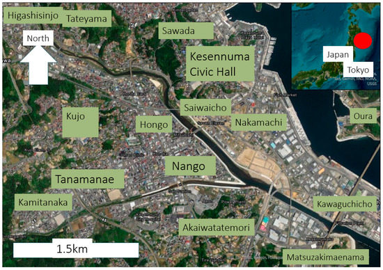
Figure 8.
Map showing the location of Kesennuma City, made using ArcGIS Pro and the ESRI World Imagery base map [24]. Location shown as red dot on the inset map.
Critical analysis of tsunami processes in Kesennuma City (Figure 8) is vital in determining tsunami-vulnerable locations for risk assessment and hazard mitigation. Both tsunami flow velocity and local inundation heights provide valuable information on tsunami behaviours and are an important factor in disaster mitigation [25,26]. To analyse tsunami impacts in Kesennuma and around Japan, civilian video footage captured during the event can be utilised. The introduction of smartphones with cameras has provided a new tool for investigating tsunami processes in localised areas of Japan and around the world. Although limited, previous studies have been undertaken investigating both flow velocity and inundation heights using videos from the Japan 2011 event. Fritz et al. [22] analysed flow velocity and inundation heights in Kesennuma Bay using a laser scanner placed in the location at which survivor videos were captured and LiDAR (light detection and ranging) to extract their results. This study found estimated flow velocities between 3 and 11 m/s and a maximum inundation height of 9 m in Kesennuma Bay. Similarly, [27] used civilian video footage to determine flow velocity and flow depth in several locations along Japan’s east coast. Flow velocity was found by estimating the movement of objects over measurable distances. They found tsunami flow velocities of 1.5 m/s in Iwaki City, 3–5 m/s in Kamaishi City, 2 m/s in Ofunato City, and 3–6 m/s in Kesennuma City. Processes used for measuring flow velocity in [25] inspired the methods for this study.
This study aims to determine how civilian video footage of a tsunami event can be analysed scientifically to gain maximum understanding of the geophysics and impact of tsunami disasters. This was investigated using the video [28] “Tsunami in Kesennuma city, ascending the Okawa River”, https://www.youtube.com/watch?v=P8qFi74k2UE, accessed 6 March 2023, captured by the civilian Mr. Kenichi Kurakami.
The research objectives for this study are as follows: (1) to assess and capture the broad impacts and tsunami characteristics observed throughout the video footage; (2) to estimate local inundation heights, by taking objects with known or calculable dimensions and measuring them against where maximum inundation can be observed in the video; (3) to estimate tsunami flow velocity in Kesennuma City by quantifying the distance and time taken for an object to travel between two measurable, known points in the video; (4) to determine whether it is possible to develop oriented imagery to display and explain the temporal progression of significant tsunami processes to increase the accuracy of video scientific analysis; and (5) to discuss the research significance and possible applications of this research for tsunami risk hazard maps and urban planning.
2. Methods
2.1. Video Selection
A significant number of videos were taken during the 2011 Tohuku earthquake and tsunami (Table 1); however, many were not suitable for use in this study. Using the internet, raw footage was sifted through to find an appropriate video for this study. The criteria for video selection were as follows (Table 1): the video had to (1) be continuous, with few-to-no cuts; (2) be long enough to see numerous tsunami processes occurring; (3) have landmarks, in order to be able to derive inundation heights and wave velocity; (4) be of acceptable quality; and (5) show the magnitude of the natural disaster.

Table 1.
Videos analysed for this study, with criteria used to examine the acceptability or non-acceptability of the video for the purposes of this study.
2.2. Video Analysis
The process of critical examination of videos involved: (1) forensic examination and scientific analysis of the selected video footage, which was reviewed numerous times in detail; (2) determination of the location the video footage, using observable features/landmarks; (3) capturing images within the video that contain significant tsunami processes, and carefully interpreting key tsunami phenomena; (4) recording key characteristics of tsunami process evidenced by the captured images; (5) determination, as precisely as possible, of the geographic coordinates of studied images using Google Maps and Street View; and, (6) determination of the camera heading for each image using the compass tool in Google Street View.
2.3. Oriented Imagery
The methods for creating an oriented imagery application have been broken into four stages: (1) pre-processing of video images; (2) creating an Oriented Imagery Catalogue; (3) creating time enabled layers; and (4) creating an oriented imagery application.
2.4. Pre-Processing of Video Images
The coordinates calculated in the previous steps were added to the screenshots by geotagging each image. These images were then uploaded to the AUT University geospatial web to be used when creating the Oriented Imagery Catalogue (Figure 9).

Figure 9.
Workflow showing the process of adding coordinates to the images captured within the video analysis process.
2.5. Creating an Oriented Imagery Catalogue
To create an Oriented Imagery Catalogue (OIC), the oriented imagery toolbox was downloaded and added to ArcGIS Pro. Within this toolbox, the “Create OIC” tool was used to create a new OIC for the Japan tsunami video imagery previously captured. Once the Japan OIC was created, images were added individually to the catalogue using the “Add Images to OIC” tool. This tool requires a number of parameters to be documented, including Imagery Type, Camera Heading, HFOV (horizontal field of view), VFOV (vertical field of view), Near Distance, and Far Distance. At this stage, only Imagery Type and Camera Heading could be filled in, as HFOV, VFOV, Near Distance, and Far Distance had not been determined. The Imagery Type “Geotagged Image” was selected for each image, and the Camera Heading was inputted with the compass direction for each image. The tool was run, and the images were placed onto the map as “exposure points” using the coordinates added previously (Figure 10).
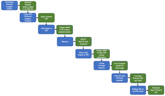
Figure 10.
Workflow showing the process of creating an oriented imagery catalogue within ArcGIS Pro.
The Far Distance and HFOV were determined for each individual image using the measure tool in ArcGIS Pro. Far Distance was measured to the farthest distance that could be clearly seen in the video. HFOV was measured as the total horizontal view that could be seen within the frame. The VFOV and Near Distance were kept as their default parameters, VFOV = 50 m, Near Distance = 0 m. Once these parameters had the correct values for each image, the “Add Images to OIC” tool was rerun.
The “Create Coverage Features” tool was used to show the view that could be seen in each of the images. The parameters were set to “From each point”, which created a coverage area for each of the images based on the parameters set previously. A time field was created within the coverage feature layer and populated with the corresponding time values from the video. Finally, the OIC was published to ArcGIS online using the tool “Publish Oriented Imagery Catalogue”.
2.6. Creating Time Enabled Layers
The early movement of the front of the tsunami wave, shown in the captured images, was digitised within ArcGIS Pro. A time field was created and populated with the corresponding video time for each digitised wave movement. Time was then enabled within the layer properties, for both the wave and the coverage feature layers. Both layers were published to ArcGIS Online as a web map (Figure 11).
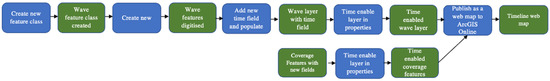
Figure 11.
Workflow showing the process of creating time-enabled wave and coverage feature layers in ArcGIS Pro.
2.7. Creating an Oriented Imagery Application
In ArcGIS online, a Japan Tsunami Experience Builder was created. Within the Experience Builder, the Oriented Imagery widget was configured using the published Japan Tsunami OIC. The timeline widget was configured using the published timeline web map containing the time enabled wave and coverage feature layers (Figure 12).
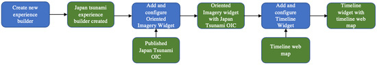
Figure 12.
Workflow showing the process of creating an oriented imagery application in ArcGIS Online.
2.8. Estimating Tsunami Flow Velocity
Estimating flow velocity was undertaken by measuring the distance and time taken for an object to travel between two measurable, known points in the video. The distance travelled was calculated by measuring the distance between two known points using imagery and the measure tool in Google Earth Pro 7.3. Time was derived using the time stamps in the footage. Velocity was calculated using the equation velocity (m/s) = distance (m)/time (s) (Figure 13).
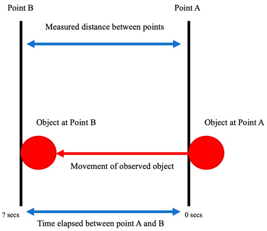
Figure 13.
Diagram explaining the process used to derive flow velocity; this was calculated by measuring the distance and time taken for an object to travel between two measurable, known points in the video.
2.9. Estimating Local Inundation Heights
Estimating local inundation heights was achieved by taking objects with known or calculable dimensions and measuring them against the maximum local inundation height observed in the video. These heights were estimated using the measurements of the average door height in Japan and the average height of a male in Japan. Google Street View imagery from 2011 was also utilised when measuring local maximum inundation height (Figure 14).
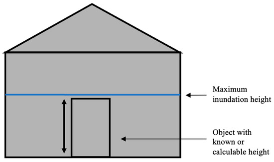
Figure 14.
Example diagram showing how an object such as a door, which has known or calculable dimensions, can be measured to derive the maximum inundation height.
3. Results
3.1. Video Analysis
The results shown in Figure 15 highlight the 10 most significant tsunami processes seen within the video footage. These video image times range from 26 s to 22 min 40 s. The key processes seen within these images begin with the receding of the Okawa River, as the water moves east towards Kesennuma Bay, exposing the riverbed (Figure 15A). Figure 15B shows the first wave siting, as it makes its way up the Okawa River, toward where the man is standing. The volume of water within the river rapidly increases, nearly reaching the top of the river levees (Figure 15C). The wave breaches the river levees, where the man was previously standing, and begins to inundate the Miniami-Kesennuma Elementary School grounds (Figure 15D). Inundation of this area continues (Figure 15E), as the tsunami wave channels through roads and streets, taking the path of least resistance over impervious surfaces (indicated by the yellow oval). In the top left of Figure 15E (indicated by the red circle), a large amount of debris from Kesennuma Bay can be seen being carried up the river by the tsunami wave. This wave of debris travels up the river passing the man, carrying with it houses, cars, and the remains of buildings destroyed by the power of the wave (Figure 15F). The wave reaches maximum local inundation height and horizontal inundation and stops moving, leaving behind a large lake of debris within the school grounds (Figure 15G). The video cuts and the water begins to recede once more, taking with it the debris brought in by the initial wave (Figure 15H). Another wave begins to ascend the river (Figure 15I) before fires break out in the distance along Kesennuma City (Figure 15J).
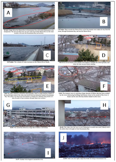
Figure 15.
The 10 most significant tsunami processes captured within the video footage, ranging from 26 s to 22 min 40 s. These images highlight key processes, including the initial receding of the river (A), the first wave siting (B), increased volume of the river (C), river breaching (D), overland inundation (E), river of debris (F), lake of debris left behind (G), receding of the first wave (H), arrival of a second wave (I), and the breakout of fires in Kesennuma City (J).
Figure 15 documents key aspects of the dynamic and rapidly changing nature of tsunamis as they interact with subaerial landscapes, in this case, within an anthropogenically modified urban landscape. Figure 15A documents a common observation with the approach of tsunamis and one that is used as an early warning signal. The river is depleted of water as it recedes ocean-wards to meet the needs of a rising tsunami wave crest. Around one minute after water recession within the river channel, a reverse flow takes place, with the river channel rapidly filling up and being utilised by the tsunami as the pathway of least resistance for the tsunami wave to move within a subaerial environment. Three minutes later, the river is at maximum capacity and the tsunami is reaching the point at which it can no longer be river-valley constrained (Figure 15C). A further 3 min is enough time for the river to be breached and for an overflow tsunami phase to begin, causing wider flooding to occur. The brown colouration of the waters shows how the water is highly sediment-charged (Figure 15D). Figure 15E begins to reveal the complex character of the extra-river channel tsunami, as it produces local lakes and moves faster through ‘artificial’ channel-ways produced by streets flanked by higher buildings. The large debris carried by the tsunami now acts as an additional erosional agent, increasing the destructive power of the tsunami. Figure 15F, an image less than 2 min from 15E in time, shows large houses and similar size ‘clasts’ being carried by the part-channel flow, part-lake flow, part-laminar, part-turbulent, part-eddy–whirlpool hydrodynamic nature of the tsunami. Figure 15G (now over 16 min into the video) reveals the ‘high tide’ mark and highest local run-up height within an urban square. The swirling and partially stagnant nature of the tsunami lake and the high concentration of eroded urban materials are visible in this image. Four minutes later (Figure 15H) reveals that this first tsunami wave is now beginning to recede, leaving behind a thick deposit of very unsorted debris. Figure 15I, at almost 22 min, reveals the onset of the second wave: unfortunately, the video footage does not show the progression of this second wave. Figure 15J reveals fires, which are a common secondary hazard associated with the primary hazard as gas leaks that become ignited. The video thus reveals itself as a powerful mechanism for the analysis of tsunami processes and their complex urban inundation phenomena/processes.
3.2. Oriented Imagery
The 2011 Tohuku Japan Tsunami–Kesennuma City: Interactive Oriented Imagery Application can be accessed through the following link: https://experience.arcgis.com/experience/2e5a1230864d4541845e520e9d221ba8/ (accessed on 9 May 2023).
Figure 16, Figure 17 and Figure 18 show the results of the configured 2011 Tohuku Japan Tsunami–Kesennuma City: Interactive Oriented Imagery Application. The configured Oriented Imagery widget allows for the selection of any coverage feature within the Oriented Imagery Map, triggering a pop-up of the corresponding image contained within that feature to appear in the widget (Figure 16). Images with overlapping coverage features can be selected.
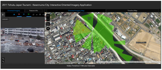
Figure 16.
The results of the configured Oriented Imagery widget with the Oriented Imagery Application. By clicking a location on the Oriented Imagery map, a red cross appears within the coverage feature, causing the corresponding image found within that coverage feature to pop up in the Oriented Imagery widget. Where there is an overlap in the coverage features, software functions can be utilised to selected and choose different images within overlapping coverage areas.
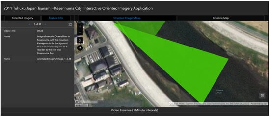
Figure 17.
The results of the configured Feature Info widget with the Oriented Imagery Application. Image information can be read through using the blue arrows in the widget. Using appropriate software function buttons features can be highlighted on the Oriented Imagery map to show the feature to which the information is relevant.
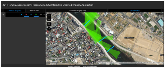
Figure 18.
The configured Timeline widget within the Oriented Imagery Application. The timeline map (connected to the Timeline widget) shows the movement of the cover features (green), and the tsunami wave (blue lines), over the map in one-minute intervals. By clicking on the cover features, a pop-up appears, containing the image description for each cover feature.
Figure 17 shows the configured Feature Info widget, which contains descriptions of the key tsunami processes visible within each of the images. By selecting appropriate software function buttons, the coverage feature connected to this information and image can be highlighted in the map.
The result of the configured Timeline widget can be seen in Figure 18. The timeline map is connected to the Timeline widget and shows the movement of the cover features (green), and the tsunami wave (blue lines), over the map in one-minute intervals. By clicking on the cover features, a pop-up appears, containing the image description for each cover feature.
3.3. Estimated Flow Velocities
Figure 19, Figure 20 and Figure 21 show the visual results for estimated flow velocity, while Table 2 shows the calculated flow velocities. Based on these calculations, flow velocities in this area range from 2.5 m/s to 4.29 m/s (Table 2).
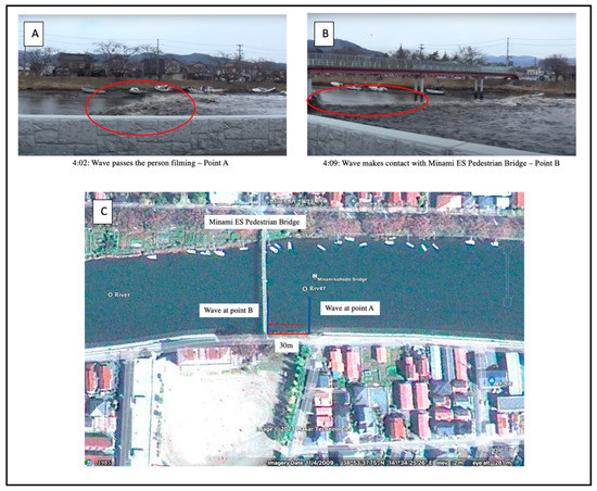
Figure 19.
The results of flow velocity estimation 1. (A) The wave passes the person filming at 4:02 into the video (red oval in the image). (B) The wave reaches Minami ES Pedestrian Bridge at 4:09 min, a time interval of 7 s between points (red oval in the image). (C) There is 30 m of distance between points A and B.
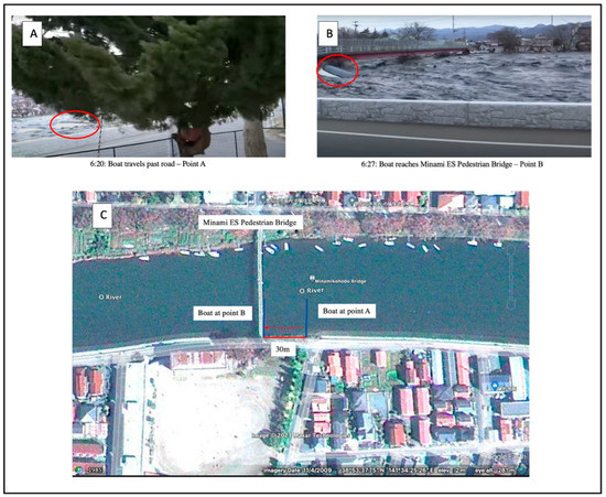
Figure 20.
The results of flow velocity estimation 2. (A) The boat passes the road at 6:20 into the video (red oval in the image). (B) The boat reaches Minami ES Pedestrian Bridge at 6:27 min, a time interval of 7 s between points (red oval in the image). (C) There is 30 m of distance between points A and B.
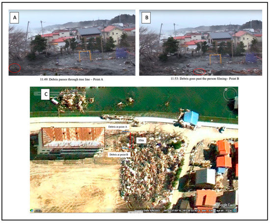
Figure 21.
The results of flow velocity estimation 3. (A) The debris passes the treeline at 11:49 into the video (red oval in the image). (B) The debris travels past the person filming at 11:53 min, a time interval of 4 s between points (red oval in the image). (C) There is 10 m of distance between points A and B.
Table 2.
Flow velocity equations using distance (m) and time (s) estimated through video analysis.
3.4. Estimated Local Inundation Maximum Height
Results of Figure 22 and Figure 23 show bridge inundation heights of 5.1 m and school building inundation heights of 2.75 m. These results show an estimated local maximum inundation height of 7.85 m in Kesennuma City.
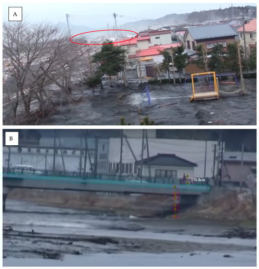
Figure 22.
(A) Image from the video showing the complete inundation of a bridge (see red oval). (B) Image from early in the video when the water level was low beneath the bridge. This was used to estimate the height of the inundated bridge by assuming the male pictured in the image was of average male height in Japan (170.8 cm), resulting in the estimated bridge height of 5.1 m.
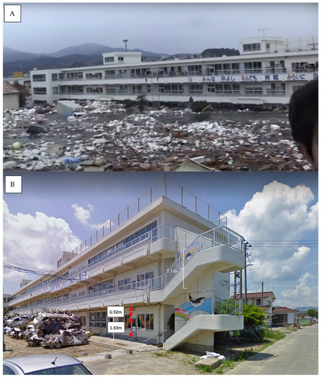
Figure 23.
(A) Image from the video showing the maximum inundation height on Miniami-Kesennuma Elementary School. (B) A Google Street View image of the school; the height was measured using the average door height in Japan (1.83 m). This resulted in a maximum building inundation height of 2.75 m.
4. Discussion
4.1. Video Analysis
The results of the video analysis process highlighted the key tsunami processes visible in the video footage (Figure 15). These processes witnessed in the video are common geophysical tsunami processes; however, understanding the specific local tsunami behaviour and movement within Kesennuma City can aid in risk management and disaster planning. The data from the video are rich and multi-dimensional. This study demonstrates the manifold ways in which the imagery can be used for qualitative and quantitative calculations and estimations, as well as to assess the rapidly changing character of tsunami inundation processes within a localised area.
4.2. Oriented Imagery
The outcome of the oriented imagery process was successful in highlighting key tsunami processes through the enablement of the Oriented Imagery widget and application (Figure 16). This widget helped to visualise and orientate the images captured from the video by linking them to coverage features on the map. Along with this, the configuration of the Timeline widget provided the ability to visualise the temporal progression of key tsunami processes seen in these images (Figure 18). The results of visualising these geophysical tsunami processes play a crucial role in influencing disaster mitigation by facilitating a deeper understanding of the risks posed by these disasters [29]. With these processes perfected, it would be possible to orientate imagery as videos are uploaded live to social media during disasters. This could be used within organisations to help quickly locate at-risk areas to aid in quicker disaster response.
4.3. Estimated Flow Velocity
Results show tsunami velocities ranging from 2.5–4.29 m/s within Kesennuma City (Table 2), in line with the study done by [27] indicating flow speeds of 3-6 m/s. Variations in velocity can be attributed to the location at which these velocities were calculated. Both flow velocities calculated within the Okawa River showed speeds of 4.29 m/s (Figure 19 and Figure 20). High speeds such as this are a result of the tsunamis tendency to maintain wave energy as it travels up stream due to a lower amount of friction [30]. In contrast to this, the flow velocity decreases to 2.5 m/s as the wave travels through the school grounds (Figure 21). The presence of trees, structures, and debris, causes increased friction and flow resistance, reducing the tsunami waves celerity and speed as it travels over land [30].
4.4. Estimated Local Inundation Heights
From these results, the estimated maximum local inundation run-up heights seen in this video is 7.85 m (Figure 22 and Figure 23). Although surveys performed by [23] indicated maximum local inundation run-up heights of 11.84 m in Kesennuma City, the height of 7.85 m calculated in this study may be the specifically localised inundation height seen in this video. Variations in local inundation heights within areas can be caused by the spatial distribution of buildings and other structures impacting the tsunamis inundation severity [31,32]. This is especially noticeable in high-density areas, as the wave will squeeze through open spaces between buildings, impacting tsunami flow depth [31,32]. Topography and vegetation are also considered to impact inundation height [33], making it important to acquire knowledge on inundation behaviours in local areas, as they may vary greatly from place to place.
4.5. Limitations and Recommendations
- Oriented imagery: Improvements can be made to the Oriented Imagery Catalogue processes within ArcGIS Pro. The VFOV (vertical field of view) was set as the default for the OIC, as there was no accurate way to estimate the VFOV visible in the images. While this was adequate for most images, the coverage features for a few may not be as accurate as hoped. This can be avoided in the future by obtaining more information about the camera being used to capture the video and the fields of view it has. Currently, time configuration within the layer properties in ArcGIS Pro only allows for certain date and time formats, e.g., yyyy-mm-dd:hh-mm-ss. Due to the times in this video not being within this date and time format, the date was correctly selected as 11 March 2011, but the times were input as video times, rather than the time of day. While this did not impact the Timeline widget’s ability to run, it did mean the time increments had to be hidden within the application to ensure no timing misinformation took place.The Oriented Imagery widget is a relatively new advancement in GIS, meaning the app configuration in this study is currently limited by the software’s capabilities. Further improvements to app configuration are recommended to increase functionality and aid in effectively communicating the timeline of key tsunami processes. As part of the OIC, the coverage map is published as a tile layer which restricts its functionality within Experience Builder. The software currently does not allow for the coverage map to be published as a feature layer. However, if this were possible, the Oriented Imagery widget and the Timeline widget could be linked within the same map in Experience Builder. This would help better communicate the temporal progression of key tsunami processes seen in the video by displaying the images over time.Intuitive connections between the Feature Info widget and the Oriented Imagery widget would also further enhance the functionality of the app. Ideally, enabling widget interaction would allow for the selection of coverage features in the Oriented Imagery map, triggering a pop-up to appear in the Feature Info widget containing information about the selected coverage feature.Finally, further improvements to the configuration of the Timeline widget should be conducted. At this stage, the time intervals between images are set to the lowest range: 1 min. This is inadequate for showing the temporal progression of the images, as the duration between them can be as low as 5 s. While this time increment was adjusted within the feature class itself, this did not translate during the configuration of the widget and requires further improvement;
- Local inundation heights: Methods used for determining local inundation heights in this study were undertaken due to the lack of high-resolution elevation data available in this area. Using high-resolution DEMs (Digital Elevation Models), DTMs (Digital Terrain Models), or DSMs (Digital Surface Models) would have been a useful tool when determining local inundation heights, as they contain accurate elevation data. However, the ALOS world 30 m digital elevation model was the only easily accessible open data source available for this study. This was unsuitable for determining accurate elevation heights within a small study area such as Kesennuma City. An alternative method to using elevation models would be to utilise the building plans of Minami-Kesennuma Elementary School or the bridge heights within this area. However, this information was unavailablemfor this study;Flow velocity: The fast flow of the tsunami and the constant movement of the person filming put limitations on the ability to execute more flow velocity calculations in this study. To increase the quantity of flow velocity calculations, it is recommended that higher quality videos and images are used, to allow for increased accuracy and reliability of results.
5. Further Analysis: Research Significance, Limitations, Tsunami Hazard Map
The analysis of civilian video footage has provided an exceptional opportunity to investigate the impact of the 2011 Tohoku, East Honshu, Japan Tsunami on Kesennuma City. These results can aid in the understanding of tsunami behaviours and help inform effective mitigation strategies in tsunami-vulnerable areas. Knowledge of local inundation heights and flow velocity within Kesennuma City can assist in determining evacuation points for future disasters by understanding tsunami flow behaviours in the area. The implementation of oriented imagery has provided a new way of visualising, communicating, and understanding the temporal progression of geophysical tsunami processes. These factors play a crucial role in influencing disaster mitigation by facilitating a deeper understanding the risks posed by these disasters. Continued studies in localised areas of Japan and around the world should be undertaken to gain further knowledge on the geophysics and impact of tsunami disasters.
The additional importance of this study is associated with the implications for wider utilisation of studies such as this one, using data created by citizens with portable mobile phone devices and ‘an eye’ for the phenomena of the moment. As smartphones with relatively high-quality video tools become more widely available to the general-public, data such as the video analysed in this study are becoming increasingly common. This situation is also true for the Pacific Islands, including Papua New Guinea, Solomon Islands, Fiji, Vanuatu, Tonga, and Samoa, all of which have experienced destructive tsunamis in the relatively recent past. Even remote village communities often have some smartphone ownership. If villagers and other citizens can become more aware of the power of video footage, particularly continuous, high-quality footage with respect to tsunamis, floods, and other geohazards, they may be more inclined to take the time to record the video footage for later utilisation and help with refining disaster reduction policies and practice. Of course, disaster situations are fraught with stress and danger; we are not advocating that people place themselves in danger, but if people are in a relative position of safety, the creation of videos, such as the one analysed within this paper, can provide invaluable data for a wide range of researchers, practitioners, and policy developers in the field of disaster risk reduction.
Figure 24 indicates pragmatic ways in which this research can be applied and further developed with respect to the understanding of localised tsunami phenomena and their impacts. We do not over-estimate the practical applications of this research, but we do offer insights into how this research can inform tsunami hazard maps within a local urban area and offer quantitative and qualitative parameters that can assist urban planners and engineers. What is apparent from this work is the importance of existing local riverine and canal channel-ways within urban space. Water-related hazards (flooding, tsunamis, storm surges) will use the zones of lowest resistance to transport water. Initial tsunami proximity to land may first draw water from the channel-ways as the tsunami wave crest builds offshore and will subsequently use the channel-ways as the primary initial means of inland inundation and water movement. This research clearly shows that this phenomenon can be easily translated as an early warning system and used to increase awareness within the local population with regards to tsunami hazard. The local inundation run-up height calculations for this mega- or high-magnitude tsunami are around 8 m; this informs urban planners and engineers of threshold levels to redesign levees, bridges, and other urban infrastructure for tsunami-vulnerable areas such as this one. The velocity calculations (2.5–4 m/s), particularly when combined with flow volumes per second within and without channels, constrain the minimum strength of buildings within the highest-risk areas. The video footage identifies areas that were first breached as the tsunami changed behaviour from valley-constrained to valley-unconstrained. This information informs future land use within the zones immediately adjacent to rivers and canals. If high levees are inappropriate defence mechanisms, it may be more useful to carefully redesign land use such that local floods result in minimum impacts. Other phenomena identified here that could be taken account of include the behaviour of transported debris/clasts and secondary fire hazards. Cars and trucks, together with weaker building structures, become easily incorporated within these high magnitude tsunamis and are effectively used as destructive erosional tools within the tsunami flow. Is there any way this hazard can be mitigated through the careful design of car parks, restrictions on road transport, and development of better early warning systems? Similarly, gas and other flammable substance storage tanks and pipeline networks should be reviewed, with a view to mitigating fire hazards.
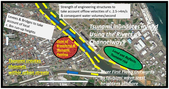
Figure 24.
Application of video analysis and calculations for local tsunami hazard map for the Nango sub-district of Kesennuma City. Yellow arrows indicate movement of channel/river flow to meet rising tsunami wave crests offshore. Blue arrows indicate reversal flow as tsunamis take advantage of low-resistance river and canal channels with respect to inland inundation. White arrows indicate the possible utilisation of streets as tsunami pathways to allow widespread inland inundation. Red oval indicates area of breaching for the 2011 tsunami, as indicated by analysed video footage. Green oval highlights one possible land use (open ground) that considers high vulnerability to tsunami inundation. The 8 m local inundation run-up height and 2.5–4 m/s flow velocities calculated in this study inform engineering and construction urban planning issues. Acknowledgments to [24] for base map.
In this research, we are aware of limitations alongside potential applications. The power of the research and research applications lies in the increasing abundance and volumes of video footage such as the one analysed within this paper. The paper is part of a thematic volume that aims to assist and inform regional development within the Papua New Guinea and wider Pacific Islands region with respect to geoscience. An increasingly widely available resource has the potential to inform geohazard discussions within a region prone to a wide number of geohazards. In the case of tsunamis, it is evident that many coastal communities within Papua New Guinea and the Pacific Islands region are vulnerable to tsunami hazards. This research clearly demonstrates the effectiveness of video footage as a means of understanding geohazard risks and impacts and, consequently, recommends that the Pacific Island countries build a library of video footage of previous and future geohazard that can be analysed and help inform communities, governments, NGOs, and similar bodies in the management of risks related to tsunamis, floods, storm surges, and related geohazards. The limitations of studies such as this include (1) the local nature of the data, limited with respect to space and time (satellite data, for example, can provide much more extensive data with respect to geographical and temporal reach); (2) the video footage is subjective to some degree, dependent on what caught the eye of the video-maker at the time of its filming—this aspect can be mitigated using numerous videos and judicious selection in the videos chosen for detailed analysis; (3) estimates of parameters such as flow velocity are undertaken in a relatively low-technology and highly practical manner, although results from this study are comparable with other studies as demonstrated above. There are techniques, such as discussed in [34] with respect to radar techniques, for flow rate calculations that have a higher level of sophistication than techniques applied in this study. We propose, however, that studies such as ours have significance from the point of view of (1) utilisation of widely available data generated by the ‘general public’ with a geoscience and geohazard lens, and analysis by geoscience experts; (2) the richness of the data for local urban and rural environments; (3) the deployment of novel analytical techniques that enhance and improve research focus, such as the interactive object orientation imagery technique (other GIS and ICT techniques will become increasingly more available and sophisticated with time); (4) the development of systematic and consistent methods and approaches to video analysis and open transparent accounts of these, as present in this study; and (5) the addition of ‘research depth’ and practical application to the results. In this case, the emphasis and advocacy of a ‘lower’ or ‘appropriate’ technology approach is far more likely to be accessible to a wide user and stakeholder group than ‘more expert systems and processes’, meaning it can better assist regions and countries such as Papua New Guinea and the Pacific Islands region. Additionally, we offer interpretations from the results of a tsunami hazard sketch map for the specific area of Nango sub-district of Kesennuma City, which have applications for many other similarly vulnerable urban areas.
Author Contributions
Conceptualization, M.G.P.; methodology, G.H..; software, G.H.; validation, C.M.-M., G.H. and M.G.P..; writing—original draft preparation, C.M.-M. and M.G.P.; writing—review and editing, M.G.P.; supervision, G.H. and M.G.P. All authors have read and agreed to the published version of the manuscript.
Funding
This research received no external funding.
Data Availability Statement
Please contact corresponding authors for data and methodology.
Acknowledgments
We strongly thank, with gratitude, Kenichi Kurakami (aka crclancy 688), who took the video footage on which this research is based.
Conflicts of Interest
The authors declare no conflict of interest.
References
- Hagen, K.; Petterson, M.G.; Humphreys, D.; Clark, N. Why Disaster Subcultures Matter: A Tale of Two Communities: How and Why the 2007 Western Solomon Islands Tsunami Disaster Led to Different Outcomes for Two Ghizo Communities. Geosciences 2021, 11, 387. [Google Scholar] [CrossRef]
- Helal, M.A.; Mehanna, M.S. Tsunamis from nature to physics. Chaos Solitons Fractals 2008, 36, 787–796. [Google Scholar] [CrossRef]
- Barman, S.K. Physics of Tsunami: Generation, Propagation and Rise of the Ocean. Int. J. Ocean. Oceanogr. 2020, 14, 169–182. [Google Scholar] [CrossRef]
- NOAA (National Oceanic and Atmospheric Administration). Tsunami Sources 1610 B.C. to A.D. 2018—From Earthquakes, Volcanic Eruptions, Landslides, and Other Causes. 2018. Available online: http://itic.iocunesco.org/images/stories/awareness_and_education/map_posters/2022_tsu_poster_20220823_a2.pdf (accessed on 9 May 2023).
- Levin, B.W.; Nosov, M. Physics of Tsunamis; Springer: Dordrecht, The Netherlands, 2009; Volume 327. [Google Scholar]
- Parwanto, N.B.; Oyama, T. A Statistical Analysis and Comparison of Historical Earthquake and Tsunami Disasters in Japan and Indonesia. Int. J. Disaster Risk Reduct. 2014, 7, 122–141. [Google Scholar] [CrossRef]
- Matsu’ura, R.S. A short history of Japanese historical seismology: Past and the present. Geosci. Lett. 2017, 4, 3. [Google Scholar] [CrossRef]
- Taira, A. Tectonic evolution of the Japanese island arc system. Annu. Rev. Earth Planet. Sci. 2001, 29, 109–134. [Google Scholar] [CrossRef]
- Yamanaka, Y.; Shimozono, T. Tsunami inundation characteristics along the Japan Sea coastline: Effect of dunes, breakwaters, and rivers. Earth Planets Space 2022, 74, 19. [Google Scholar] [CrossRef]
- Ando, M. Source mechanisms and tectonic significance of historical earthquakes along the Nankai Trough, Japan. Tectonophysics 1975, 27, 117–140. [Google Scholar] [CrossRef]
- Sangawa, A. Evidences of paleo-earthquakes at archaeological sites. In Proc. Jt. Meet. US/Jpn. Coop. Program Dev. Util. Nat. Resour. Panel Earthq. Predict. Technol., 9th ed.; Geogr. Surv. Inst.: Tsukuba, Japan, 1994; pp. 137–143. [Google Scholar]
- Fukao, Y.; Furumoto, M. Mechanism of large earthquakes along the eastern margin of the Japan Sea. Tectonophysics 1975, 25, 247–266. [Google Scholar] [CrossRef]
- Rikitake, T.; Aida, I. Tsunami hazard probability in Japan. Bull. Seismol. Soc. Am. 1988, 78, 1268–1278. [Google Scholar]
- Woessner, J.; Farahani, R.J. Tsunami inundation hazard across Japan. Int. J. Disaster Risk Reduct. 2020, 49, 101654. [Google Scholar] [CrossRef]
- Norio, O.; Ye, T.; Kajitani, Y.; Shi, P.; Tatano, H. The 2011 eastern Japan great earthquake disaster: Overview and comments. Int. J. Disaster Risk Sci. 2011, 2, 34–42. [Google Scholar] [CrossRef]
- Fujii, Y.; Satake, K.; Sakai, S.; Shinohara, M.; Kanazawa, T. Tsunami source of the 2011 off the Pacific coast of Tohoku earthquake. Earth Planets Space 2011, 63, 815–820. [Google Scholar] [CrossRef]
- Lay, T.; Kanamori, H. Insights from the great 2011 Japan earthquake. Phys. Today 2011, 64, 33–39. Available online: https://authors.library.caltech.edu/28770/1/Lay2011p16763Phys_Today.pdf (accessed on 9 May 2023). [CrossRef]
- Japan Meteorological Agency. About the “2011 off the Pacific Coast of Tohoku Earthquake” (28th Report). 2011. Available online: https://www.jma.go.jp/jma/press/1103/25b/201103251730.html (accessed on 9 May 2023).
- Nakahara, S.; Ichikawa, M. Mortality in the 2011 tsunami in Japan. J. Epidemiol. 2013, 23, 70–73. [Google Scholar] [CrossRef] [PubMed]
- Tsuji, Y.; Takahashi, T.; Imai, K. Comparison of tsunami height distributions of the 1960 and the 2010 Chilean earthquakes on the coasts of the Japanese Islands. AGU Fall Meet. Abstr. 2010, 2010, G33A-0832. [Google Scholar]
- Fritz, H.M.; Petroff, C.M.; Catalán, P.A.; Cienfuegos, R.; Winckler, P.; Kalligeris, N.; Weiss, R.; Barrientos, S.E.; Meneses, G.; Valderas-Bermejo, C.; et al. Field survey of the 27 February 2010 Chile Tsunami. Pure Appl. Geophys. 2011, 168, 1989–2010. [Google Scholar] [CrossRef]
- Fritz, H.M.; Phillips, D.A.; Okayasu, A.; Shimozono, T.; Liu, H.; Mohammed, F.; Skanavis, V.; Synolakis, C.E.; Takahashi, T. The 2011 Japan tsunami current velocity measurements from survivor videos at Kesennuma Bay using LiDAR. Geophys. Res. Lett. 2012, 39, L00G23. [Google Scholar] [CrossRef]
- Mikami, T.; Shibayama, T.; Esteban, M.; Matsumaru, R. Field Survey of the 2011 Tohoku Earthquake and Tsunami in Miyagi and Fukushima Prefectures. Coast. Eng. J. 2012, 54, 1250011-1–1250011-26. [Google Scholar] [CrossRef]
- Google Earth Pro V 7.3. (April 11, 2009). Kesennuma City, Map View, Japan. 38°53′37.75″ N, 141°34′25″ E, eye alt 281m. Available online: https://www.google.com/maps/@38.911219,141.5828318,9087m/data=!3m1!1e3?authuser=0&entry=ttu. (accessed on 2 June 2023).
- GNS Science. GNS Science Consultancy Report 2013/131—Tsunami Report. 2013. Available online: https://www.civildefence.govt.nz/assets/Uploads/publications/GNS-CR2013-131-Tsunami-Report-4-Tsunami-Modelling.pdf (accessed on 3 May 2023).
- Ramadan, K.T. Near- and far-field tsunami waves, displaced water volume, potential energy and velocity flow rates by a stochastic submarine earthquake source model. Nat. Hazards Earth Syst. Sci. 2018, 1–28. [Google Scholar] [CrossRef]
- Foytong, P.; Ruangrassamee, A.; Shoji, G.; Hiraki, Y.; Ezura, Y. Analysis of Tsunami Flow Velocities during the March 2011 Tohoku, Japan, Tsunami. Earthq. Spectra 2013, 29 (Suppl. S1), 161–181. [Google Scholar] [CrossRef]
- Clancy688. Tsunami in Kesennuma City, Ascending the Okawa River [Video]. YouTube. 8 April 2013. Available online: https://www.youtube.com/watch?v=P8qFi74k2UE (accessed on 1 October 2022).
- Goda, K.; Song, J. Uncertainty modeling and visualization for tsunami hazard and risk mapping: A case study for the 2011 Tohoku earthquake. Stoch. Environ. Res. Risk Assess. 2016, 30, 2271–2285. [Google Scholar] [CrossRef]
- Adityawan, M.B.; Roh, M.; Tanaka, H.; Mano, A.; Udo, K. Investigation of tsunami propagation characteristics in river and on land induced by the Great East Japan Earthquake 2011. J. Earthq. Tsunami 2012, 6, 1250033. [Google Scholar] [CrossRef]
- Sadashiva, V.K.; Wang, X.; Lin, S.L.; Lukovic, B.; Heron, D.W.; Suppasri, A. Quantifying effects of explicit representation of buildings in tsunami inundation simulations. Int. J. Disaster Risk Reduct. 2022, 81, 103277. [Google Scholar] [CrossRef]
- Wang, X.; Power, W.; Lukovic, B.; Mueller, C.; Liu, Y. A pilot study on effectiveness of flow depth as sole intensity measure of tsunami damage potential. In Proceedings of the 2020 New Zealand Society for Earthquake Engineering Annual Technical Conference, Wellington, New Zealand, 22–24 April 2020. [Google Scholar]
- Kaiser, G.; Scheele, L.; Kortenhaus, A.; Løvholt, F.; Römer, H.; Leschka, S. The influence of land cover roughness on the results of high resolution tsunami inundation modeling. Nat. Hazards Earth Syst. Sci. 2011, 11, 2521–2540. [Google Scholar] [CrossRef]
- Wang, Y.; Imai, K.; Mulia, I.E.; Ariyoshi, K.; Takahashi, N.; Sasaki, K.; Kaneko, H.; Abe, H.; Sato, Y. Data assimilation using high-frequency radar for tsunami early warning: A case study of the 2022 Tonga volcanic tsunami. J. Geophys. Res. Solid Earth 2023, 128, e2022JB025153. [Google Scholar] [CrossRef]
Disclaimer/Publisher’s Note: The statements, opinions and data contained in all publications are solely those of the individual author(s) and contributor(s) and not of MDPI and/or the editor(s). MDPI and/or the editor(s) disclaim responsibility for any injury to people or property resulting from any ideas, methods, instructions or products referred to in the content. |
© 2023 by the authors. Licensee MDPI, Basel, Switzerland. This article is an open access article distributed under the terms and conditions of the Creative Commons Attribution (CC BY) license (https://creativecommons.org/licenses/by/4.0/).