Dynamic Prediction of Longitudinal Settlement of Existing Tunnel Using ConvRes-DLinear Model with Integration of Undercrossing Construction Process Information

Abstract

Undercrossing construction can cause severe structural deformation of the above existing tunnel in operation. The induced longitudinal differential settlement between the segments can pose a huge risk to running subways, hence it is of great importance to monitor and predict the settlement. Within this study, a Wireless Sensor Network (WSN) system was implemented to obtain hourly monitoring data of settlement from the very beginning of undercrossing to post construction period. An improved direct multi-step (DMS) forecasting model called ConvRes-DLinear is proposed, which fuses monitoring data with time and process encoding bias to deeply extract and learn temporal correlation of time series. A residual LSTM model is also constructed to compare the accuracy of the improved DLinear model. The training and testing experiment on the monitoring data of longitudinal settlement obtained by WSN system shows that the ConvRes-DLinear model with time and process encoding bias performs surprisingly well with a minimum prediction error. The features of the proposed model are discussed to make the results explainable. The monitoring system and time series forecasting model proposed in this study have a guiding significance for the monitoring and prediction of longitudinal differential settlement of tunnels under environmental disturbance.

1. Introduction

The accurate prediction of tunnel lining deformation is a critical task for ensuring the safe and efficient operation of subway systems. The ability to predict deformation enables maintenance personnel to quantify the service life of the structure, develop appropriate repair plans, and ultimately ensure passenger safety. However, accurate prediction of tunnel lining deformation is a challenging task that requires a deep understanding of the underlying factors contributing to deformation and the development of sophisticated prediction models. In practical situations, it is often impossible to anticipate structural deformations due to a multitude of complex factors. As a result, numerical simulations that are conducted often only occur during the design stage or post-accident review and analysis, leading to an absence of accurate models and techniques for predicting tunnel lining deformation during operation [1,2,3,4,5]. Achievement of accurate prediction of deformation in tunnel lining structure is therefore an urgent challenge that must be tackled to ensure continued safe and reliable operation of subway systems.

The advent of deep learning has opened up new avenues for constructing predictive models by leveraging the ability to extract implicit features and optimize parameters through gradient descent, thereby enabling efficient and accurate modeling of complex structural deformations, such as those encountered in the case of tunnels. While the deep learning models may not capture exact laws governing structural deformation, they still offer a pragmatic approach for approximating real-world scenarios by utilizing input variables to generate output results. This effective yet uncertain approach assumes significant importance for subway operations, where timely and accurate predictions of structural changes can facilitate efficient and safe operations. Despite its limitations, deep learning-based approaches can expedite the modeling process and offer valuable insights into the complex behavior of underground tunnels.

To develop a robust predictive model to estimate structural deformation in tunnels, a comprehensive understanding of the problem domain and the requisite inputs and labels is critical [6,7,8]. Constructing an accurate data set is a major challenge, as it often involves extensive effort and substantial resources. However, with the advent of advanced monitoring techniques, we have access to vast amounts of data, which can be used to generate a temporal sequence data set of structural deformation. In this context, the input data consists of historical monitoring datasets, and the output labels represent the predicted structural deformation for specific or multiple locations in the future [9,10,11]. Deep learning technology provides a powerful framework for constructing a predictive model that can effectively approximate the laws of structural deformation by extracting implicit features and systematically optimizing the model parameters to minimize the prediction error. What’s more, environmental geological information is fused into traditional physical models through empirical or physical parameters. However, in deep learning, the geological information can also be incorporated into neural networks as features or biases, serving as prior knowledge for structural deformation learning. This integration will aid neural networks in capturing the patterns of structural deformation. Then the learning process can involve the application of convex optimization methods, such as gradient descent, to fit the deformation pattern of the tunnel. Although the features learned by deep learning algorithms are not always interpretable in the traditional sense, the output results generated by these models often provide accurate estimates of real-world situations. In practice, this fuzzy yet effective approach has significant practical implications for subway operations. By leveraging the power of deep learning to build end-to-end predictive models, subway operators can better anticipate structural deformations and take proactive measures to mitigate any potential safety risks. Moreover, by continually expanding the training set, enriching geological information representation and dynamically fine-tuning the model, we can enhance the accuracy and reliability of our predictions, thereby optimizing the performance of the subway system [12,13].

This paper is based on the above two main points: the advanced deep learning models that can integrate environmental geological information and modern monitoring devices [14] for shield tunnel deformation, to construct and train an engineering-applicable structural deformation prediction model. Such a model can be directly deployed on the monitoring center platform of subway operation [15,16], which has practical significance for the healthy operation of the subway. The structure of this paper is as follows: Section 1 introduces the subway structural deformation prediction; Section 2 introduces the current time series prediction models, the model we adopted, and our model improvements; Section 3 describes the instruments used to collect the dataset and the structure of the collected dataset; Section 4 provides a detailed introduction to our data collection methods and data sets based on the longitudinal settlement deformation of tunnels in the Hangzhou subway, used to predict the transverse convergence deformation of adjacent tunnel segments; Section 5 presents the training of the time series prediction model based on the project data, followed by a comparison of multiple models; Section 6 concludes with the forecast and future prospects of structural deformation prediction.

2. Longitudinal Settlement Prediction Model Architectures

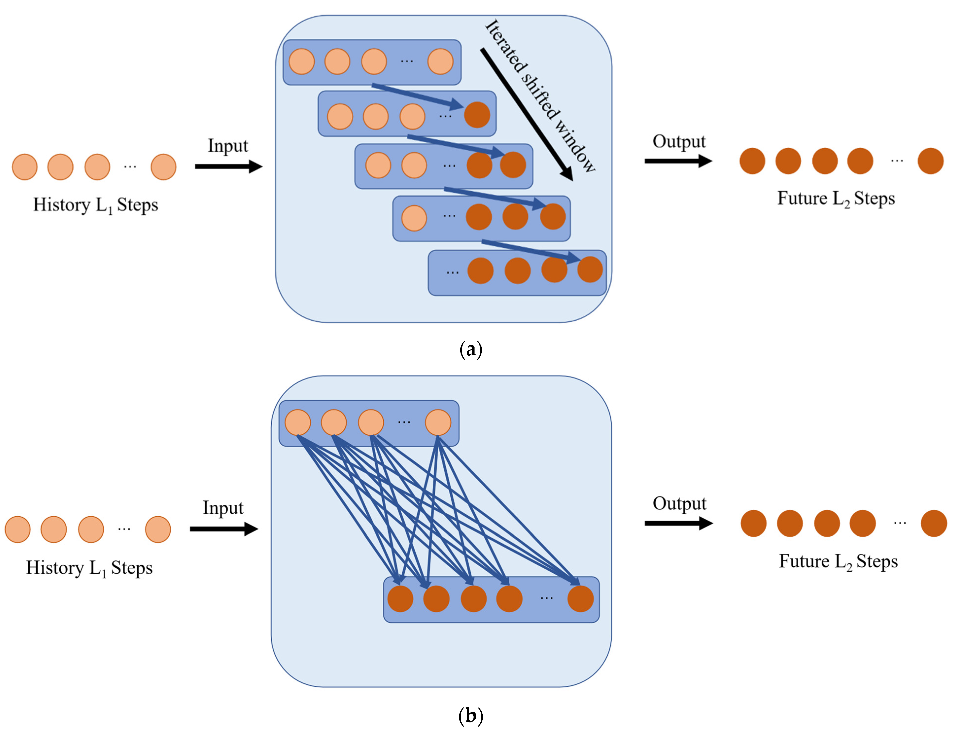
Given the importance of longitudinal settlement time series prediction, it is crucial to consider the appropriate approach to obtain accurate results. Two common methods of time series prediction include single-step iterative prediction [17] and multi-step direct prediction [18], as detailed in Figure 1. To address these methods, deep learning techniques have been employed and have promoted several advancements in research. Prior studies have employed machine learning approaches, such as ARIMA [19], which use multivariate fitting to analyze time series data. While these methods are useful for specific datasets with significant periodic patterns, such as sine waves, real-world data may prove more challenging to analyze. In recent years, deep neural networks have emerged as powerful alternatives for time series prediction. Subfields of deep learning such as RNN [20,21] and transformer [22,23,24,25,26] have produced significant results in this area. Thus, this study provides a brief overview of these validated and classic models.

RNN models are a type of neural network with a sequential structure that can capture historical patterns of variation over a period of time in order to predict future developments over a short time window. A representative example of RNN models is LSTM, a long short-term memory network, in which the three gates, namely the forget gate, the input (or choose) gate, and the output gate, can effectively fuse the historical state, the current input, and the current hidden state, to predict the future. However, RNN-like models generally suffer from two problems. First, multiple time steps share weight parameters in model training, making it difficult to optimize model performance when dealing with long-term dependencies. Second, the sequential structure of RNN models prevents efficient leveraging of GPU parallelism, leading to much longer training times. As a result, the field of transformer models has become increasingly mainstream as an alternative to RNN models.

Transformers have gained much popularity in the field of deep learning due to their excellent performance in attention mechanism, which determines the relevance between input and output elements by assigning weights to them. The original attention mechanism utilizing inner product has effectively captured long-range correlations in sequence data, which is highly valuable in natural language processing. Subsequent studies have developed several variations of the attention mechanism, such as generating learnable weight matrices by linearly mapping queries. However, the significance of this attention mechanism for time series prediction remains unclear, despite its various novel forms, as we are only multiplying and summing hidden variables to obtain their numerical correlations. Furthermore, in the field of structural deformation prediction, there may not be a strong correlation between the present deformation and one that happened a long time ago, implying that computing correlations between the numerical values at each time point may not be reasonable. Some models have attempted to calculate correlations in the frequency domain through Fourier transformation, which is somewhat reasonable, but the prediction performance of these models is still unsatisfactory.

Recently, a new paradigm for time series prediction, called DLinear, has been proposed. As its name suggests, this model only uses a few linear mappings, with fewer parameters, yet it achieves stunning performance in predicting long time steps. It outperforms transformer based prediction models in publicly available datasets related to electricity, exchange, traffic and weather. In this paper, we propose ConvRes-DLinear, an improved version of DLinear in aspects of feature input, feature fusion and residual path. 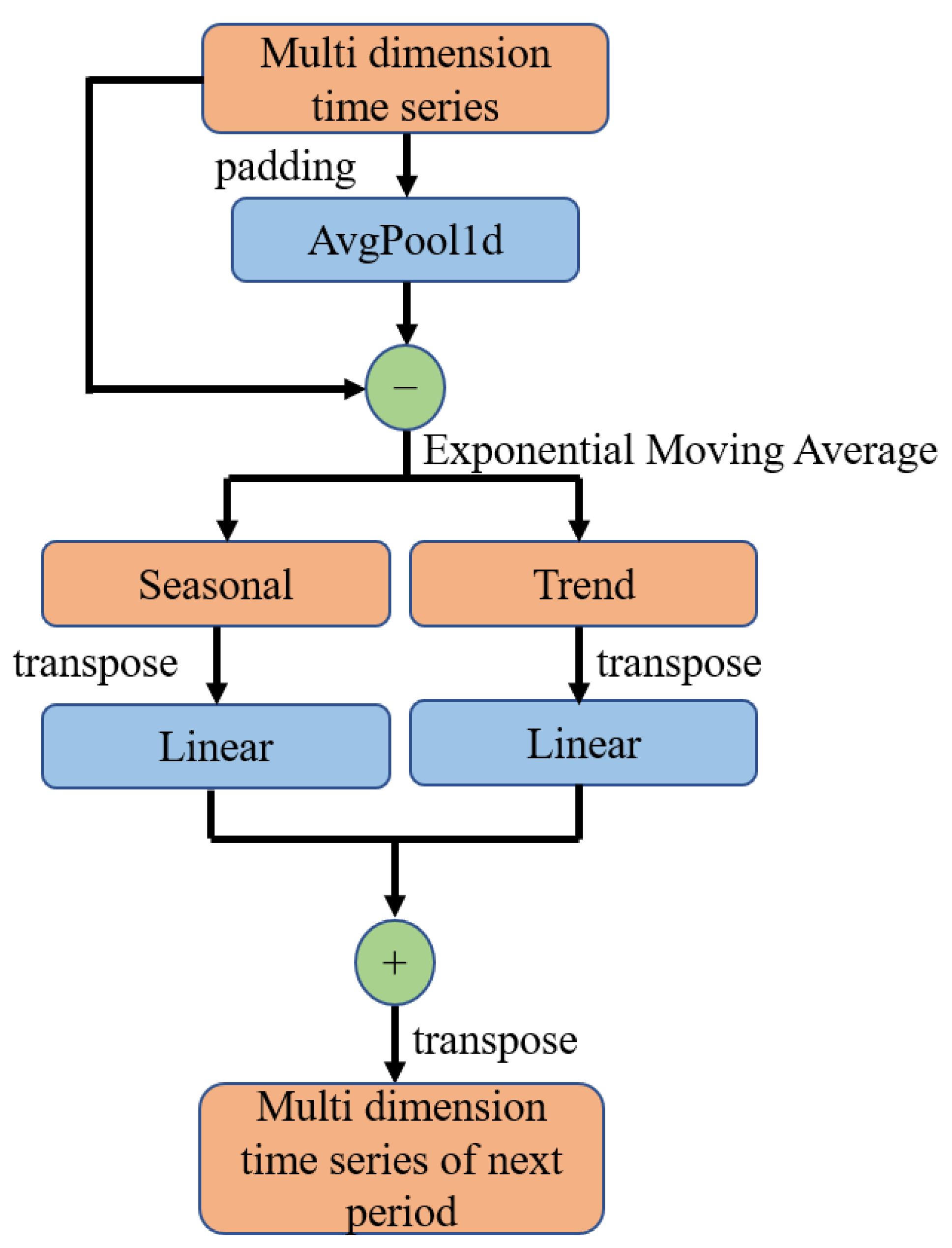Figure 2 shows the original structure of DLinear, which is simple and direct.

The data flow of DLinear is clear. Firstly, the time series data after average pooled is exponentially smoothed, divided into fluctuation data with a certain regularity and monotonic data without regularity, and then overlapped after two linear mapping layers. Finally, the output is the target data to be predicted, and the size of the linear mapping matrix is adjusted to adjust the time step. It is worth noting that the two linear mapping matrices in DLinear are different from the general feature mapping matrices. They directly map on the temporal dimension after transposing the time-series data. This is a very novel innovation because traditional neural networks such as multi-layer perceptron and the popular transformer all scale the input sequence dimension, while DLinear directly transposes the input data, treats the time dimension as its new feature dimension, and achieves astonishing results with just two simple linear mapping matrices. Moreover, this simplicity provides ample room for improvement based on DLinear. It also prompts us to consider whether continuously increasing the model parameters and the number of layers is really necessary for simple time-series prediction tasks.

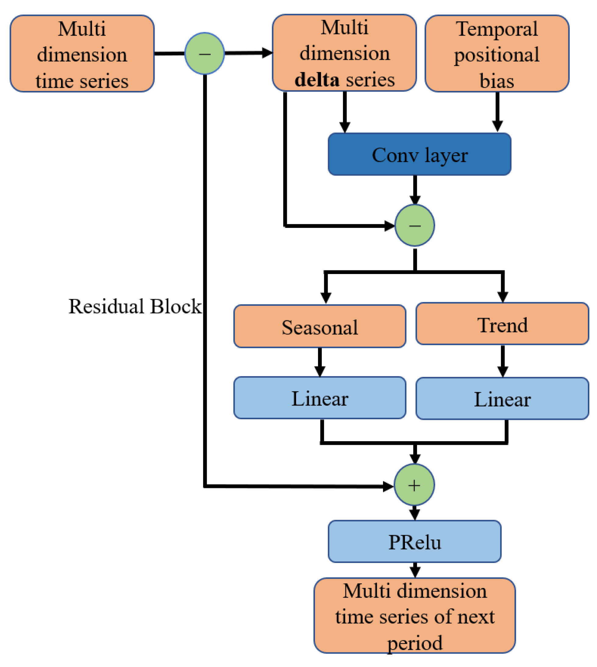
In this simple yet effective framework of DLinear, we can make various improvements based on the actual geological meaning of structural deformation prediction. The ConvRes-DLinear proposed in this paper improves three aspects: (1) Instead of directly inputting time series data, we determine the starting time of each time period and calculate the increment during this period as the input to the model. At the same time, the data value at start time is directly added to the PRelu activation function in the form of residuals, and this method of calculating the difference will replace the data normalization method [27]. (2) We incorporate temporal and geological information into the input as bias, which can be customized when preparing the dataset and can therefore serve as a paradigm for constructing a structural deformation dataset [28]. In later sections, you can see that we provide a method for defining additional geological information for specific monitoring projects. (3) We add a one-dimensional convolution layer before the exponential average of geological information, aiming to fuse the features of both the input time sequence and geological information. The parameters of one-dimensional convolution are learnable, and it will provide more parameter redundancy than one-dimensional pooling for feature extraction. In summary, the addition of Residual blocks and convolutional layers is the source of the name ConvRes-DLinear. The architecture of ConvRes-DLinear is shown in Figure 3. The PRelu function is described in Equation (1):

$$y_i=\max (0,y_i)+0.25\times \min (0,y_i)$$

(1)

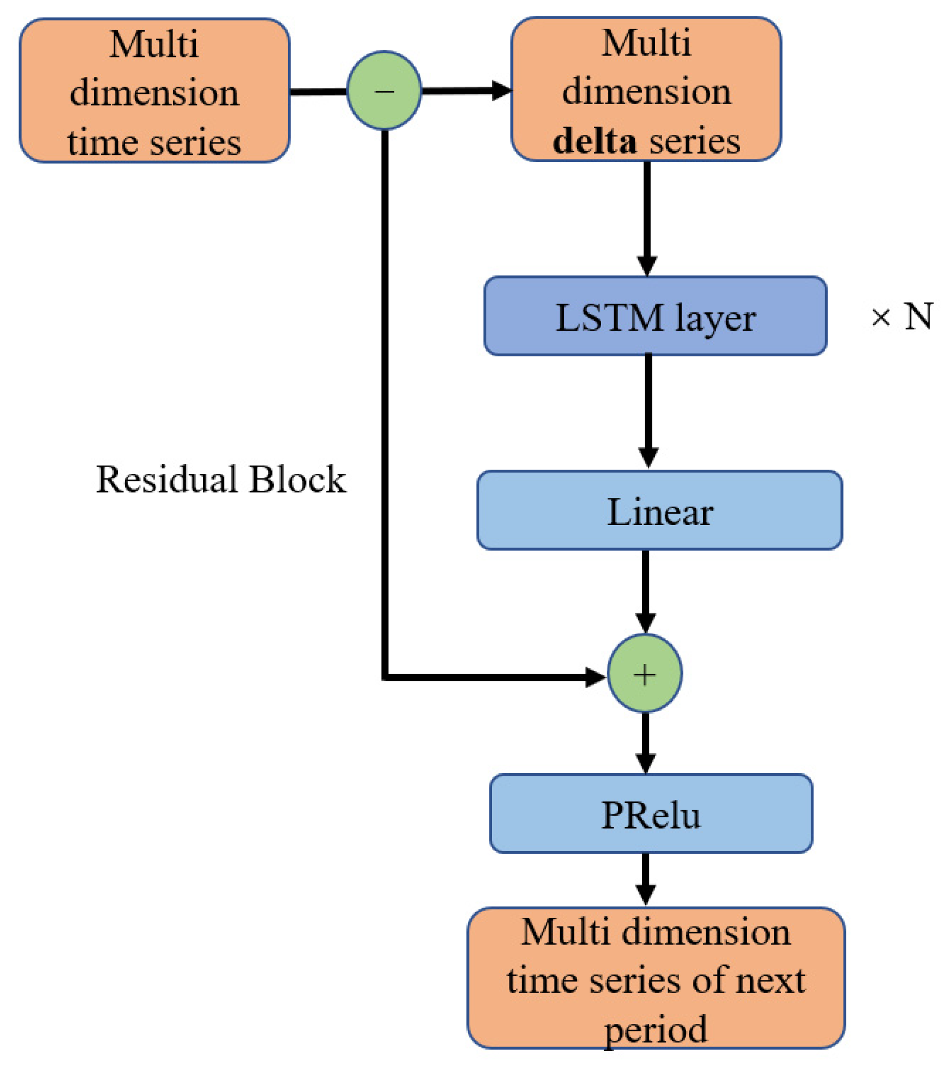
In addition, RNN based model such as LSTM is comparable to DLinear in aspects of model structure complexity and parameter quantity, and the sliding window mechanism exhibits a similar data flow pattern. To authors’ best knowledge, no comparison can be found between RNN based model and DLinear based model on structural health monitoring data prediction task, therefore, we use LSTM as a benchmark to train and compare it with DLinear based model on our self-collected dataset. we also made improvements to the LSTM hidden variable mapping, which we called time series prediction residual path. Specifically, we eliminated the normalization operation that LSTM performs on input data at each time step, and instead, added the structural deformation increment for a period of time as a residual input. This is added before the activation function of the LSTM hidden layer was applied. This improvement is similar to the first improvement we made to DLinear. The architecture of improved LSTM is shown in Figure 4. The comparison between the two RNN based model will help illustrate the effect of the proposed residual path, which shrinks the prediction time step for LSTM and probably help LSTM perform better.

3. Creation of Dataset for Time Series Prediction of Structural Deformation

In the civil engineering field, there are various types of structural deformation. To train a high-precision longitudinal settlement deformation prediction time-series model, the constructed dataset must meet certain conditions, namely, sufficient data quantity, continuous data, reliability, and accuracy. The number of datasets collected through manual monitoring is limited. Moreover, in the operating tunnel, structural deformation monitoring can only be carried out at night, and this dependence on monitoring personnel’s work status inevitably leads to large errors in the reliability and accuracy of datasets. To construct datasets that meet the requirements, it is essential to seek the help of automatic monitoring equipment. Thanks to the development of WSN [29] and MEMS [30], installing high-precision, fully automated instruments for collecting a large amount of monitoring data in a limited space during tunnel operation has become possible. We used VDMS, i.e., the vertical displacement monitoring system, to construct a longitudinal settlement deformation time-series dataset in the shield tunnel. This is a new MEMS-based longitudinal settlement monitoring device, and its hardware construction is shown in the Figure 5.

The VDMS is a linked rod structure, with each rod containing MEMS three-axis accelerometers installed internally. These rods are connected to form a system for monitoring longitudinal deformation in shield tunnels. The three-axis accelerometers within each rod sense changes in numerical values along three orthogonal axes due to the force of gravity, enabling real-time detection of the spatial orientation of the rods and calculation of longitudinal deformation within each rod. When multiple sensor rods are combined, continuous analysis of each rod’s orientation changes can be conducted, enabling ongoing calculation of longitudinal settlement deformation in the monitoring area. Endpoint rods can be set as point 0, with zero longitudinal settlement, allowing for continuous calculation of longitudinal settlement in the entire monitored section by the VDMS. Given the assumption that the inclination change and the cell length of the ith cell of the VDMS are known saying Δφ_i and L_i, the settlement of the monitoring section can be measured and calculated sequentially cell by cell. Then the settlement curve can be obtained (Figure 6). Supposing that the settlement y₀ at the start is known, the settlement y_p at the point x_p is equal to Equation (2).

$$y_p=y_0+{\displaystyle \sum _{i=1}^{k-1}(L_i\sin \mathsf{\Delta }{\phi }_i)}+(x_p-{\displaystyle \sum _{i=1}^{k-1}{L}_i})\sin \mathsf{\Delta }{\phi }_k$$

(2)

where k means that the point x_p is located within the kth cell and L_i can be referred to the real length of the rod, which is 2000 mm.

The accuracy of the monitoring data obtained by this instrument has been demonstrated previously, ensuring the data is reliable and of high precision. In addition to satisfying the requirement for high precision monitoring, VDMS also meets the reliability needs for massive data transmission. A wireless gateway is connected to the end of VDMS, allowing the monitoring data to be sent to the base station at a user-defined frequency, with a frequency as high as 1 min, thus collecting a continuous stream of massive longitudinal deformation data [31].

4. Construction of Data Set Based on a Monitoring Project

In this article, our dataset of longitudinal settlement and deformation of shield tunnel comes from the monitoring of Hangzhou Metro Line 4. The purpose of the project is to monitor the impact of shield tunneling on the settlement of the existing tunnel. From top to bottom, the geological layers consist of gravelly fill, sandy silt, muddy silty clay, medium sand and pebble. Both tunnels are located in a compressible and collapsible layer of muddy silty clay. The layer is quite moist, moderately dense, and contains fragments of mica. It locally includes thin layers of clay and a small amount of silt. The static cone penetration resistance ranges from 1.81 to 4.40 MPa, with an average value of 3.12 MPa. The side friction ranges from 26.8 to 53.6 kPa, with an average value of 42.8 kPa, as measured by static cone penetration tests. The standard penetration test ranges from 4.0 to 13.0 blows, with an average value of 8.4 blows. The layer is partially distributed, with thickness ranging from 0.9 to 8.7 m, and the top of the layer is buried at depths ranging from 2.2 to 9.8 m, with elevations ranging from −4.27 to 2.21 m. This layer belongs to moderately compressible soil with poor engineering performance. It is prone to collapse and deformation, as well as the occurrence of piping, sand flow, and vibration-induced liquefaction phenomena. 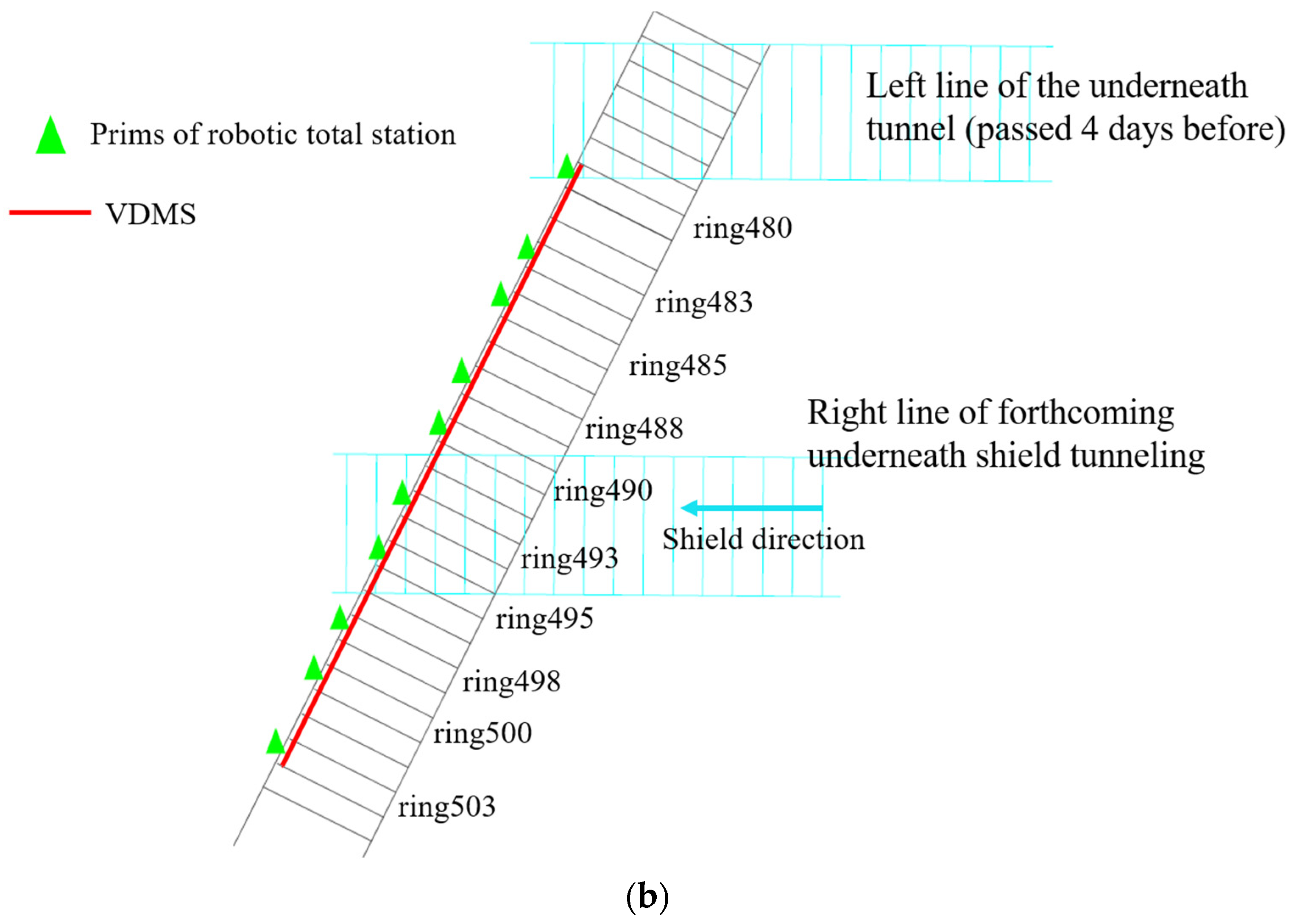The environmental geological condition is shown in Figure 6a. The minimum distance between the new and existing tunnels is only 4.46 m, and the existing tunnel was not reinforced in advance. Therefore, the existing tunnel is prone to significant uneven settlement in the crossing area. The planar relationship between the monitoring tunnel and the tunnel being crossed is shown in Figure 6b. The new tunnel passes under the existing tunnel at an angle of 65°, and the section of the existing tunnel is a single circular shield tunnel, using staggered joint reinforced concrete segments with a diameter of 6.2 m, a segment thickness of 0.35 m, and an annular width of 1.2 m. There are two crossing tunnels, and the left line was already crossed the existing tunnel four days before VDMS started monitoring, with the crossing point facing the existing tunnel at ring 475; the right line crossed the existing tunnel 26 days after VDMS started monitoring, with the crossing point facing the existing tunnel at ring 490. Both crossing tunnels have a diameter of 6.9 m. The VDMS monitoring section is 28 m long and has 14 measurement units, installed between ring 480 and ring 503 of the existing tunnel, and a data transmission gateway is installed at ring 479. 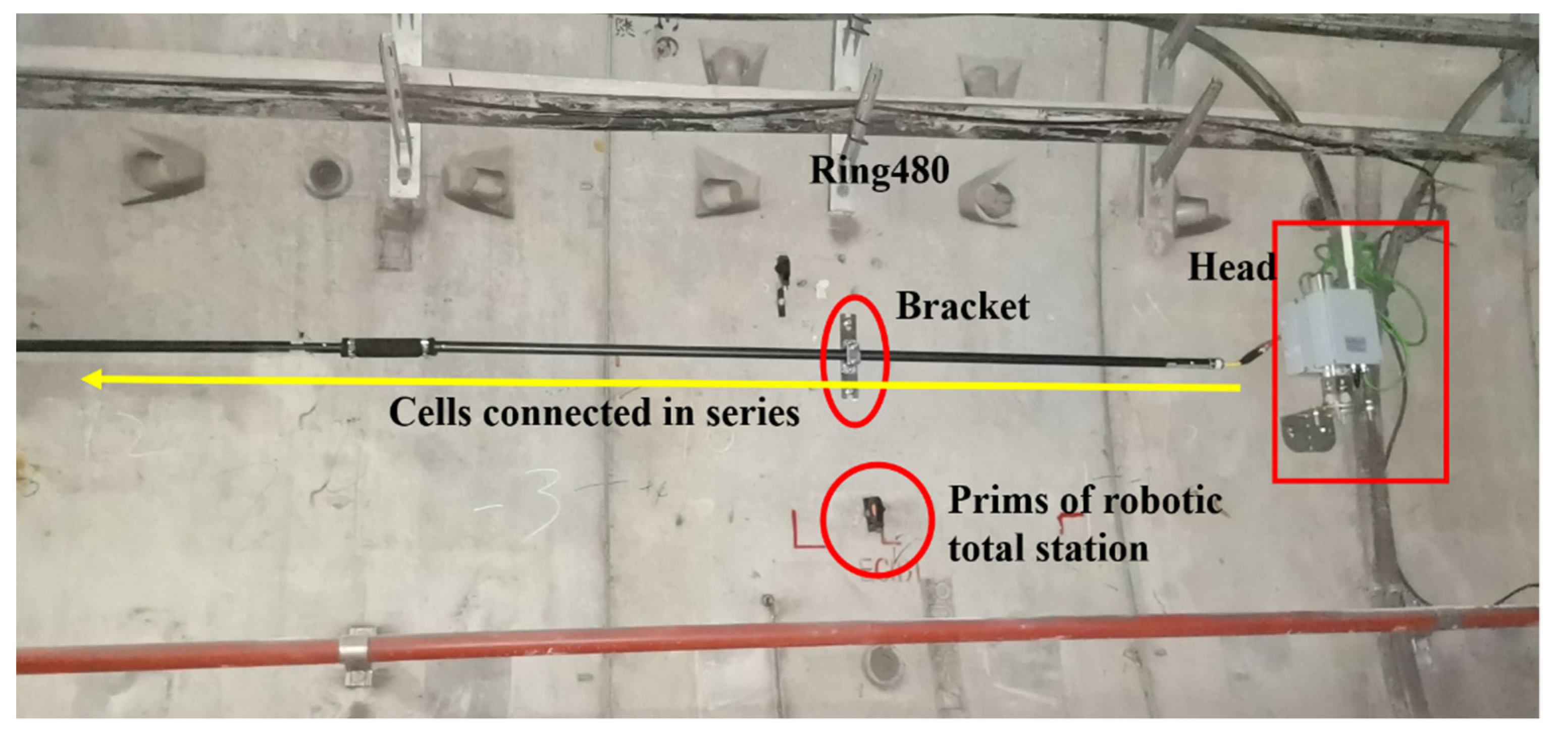Figure 7 is a photo of VDMS after installation at the site.

Our time series dataset consists of two parts: the first part is the data obtained from VDMS monitoring, and the second part is the environmental geological time series information. Since the tunnel is situated in a soft clay layer, the construction disturbances during excavation will have an impact on the properties of the soil and consequently affect the existing tunnel above. However, quantifying or encoding the changes in soil properties directly is challenging. Therefore, we collected the construction process information of the under-crossing tunnel and used it as a feature input. This construction process information can implicitly represent the environmental geological information. In this case, shield machine’s schedule for the under-crossing operation obtained from the construction party is applied. 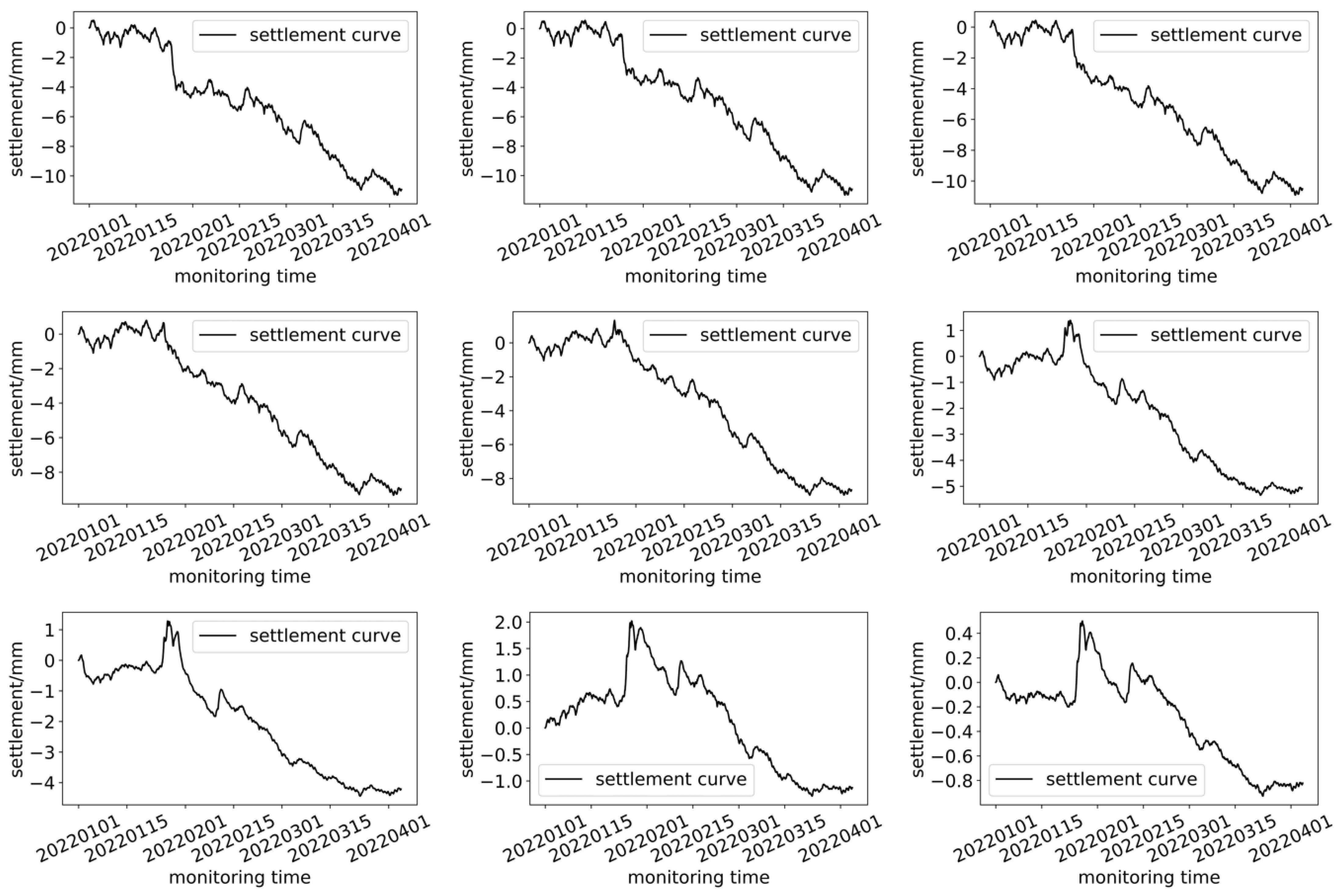The acquisition of the second part of process data succinctly constructs the geological information of the input time series model, as mentioned in the construction of ConvRes-DLinear in Section 2. VDMS began collecting data on 1 January 2022, and continued until 4 April 2022, with a monitoring frequency of one hour. All 2247 pieces of monitoring data are continuous and uninterrupted. In addition, only the settlement data of certain rings calculated using Equation (2) are retained in this dataset. These rings are sections 480, 483, 485, 488, 490, 493, 495, 498, 500, and 503. Ring 503 is set as the starting point, so the settlement of ring 503 is set to 0 at every sampling time during the monitoring period, and the settlement of other rings is calculated based on segment 503. Figure 8 shows the visualization of the data changes.

The second part of the data, i.e., the schedule for the shield machine’s under-crossing operation, is very simple. It tells us that the excavation began on 9 January and the shield machine arrived directly underneath the VDMS monitoring section on 26 January, and 50 sections were crossed on February 8, indicating that the shield machine had moved completely away from the area of interest. In comparison with the shield machine under-crossing time provided by the construction party, we can see obvious uplift and post-construction settlement of the overlying tunnel (i.e., the tunnel we are monitoring) in Figure 8.

It is worth noting that in time series prediction tasks, input of environmental variables is often a crucial variable. The independent and dependent variables are often directly related, and therefore, a time series prediction model can be trained and modeled directly. However, the environmental variables often play an important role in the changes of the independent and dependent variables. Especially in the case of tunnel subsidence under large environmental disturbances, it is often caused by changes in soil pressure, groundwater infiltration pressure, and overlying soil pressure. If the time series prediction dataset can adequately consider these environmental data, that is, consider incorporating appropriate geological information during model training, it will make the model more robust and effective. Additionally, when deploying and applying time series prediction neural network models, we can gather the same format of geological information and input it into the model along with the independent variables for prediction, thus forming a closed loop for the training and deployment of a high-precision time series prediction model.

Now that the geological information has been collected, a new problem has arisen, which is how to represent geological information as information that can be input into the model. Neural network inputs are in the form of vectors, so we also need to transform this geological information into suitable vectors for input. In various variants of transformer, time-series information is represented by a position encoding matrix that can be learned or fixed, and some works also express information representing processes as different coefficients of position encoding. However, our model is not a transformer based structure but a DLinear based, which is unsuitable to include positional encoding as the input bias. At the same time, we do not intend to extend the feature dimensions of deformation monitoring data through an embedding layer similar to NLP. Therefore, we consider how to transform geological information into a numerical representation, which can be directly input into the model. In this paper, we refer to the expression form of the sigmoid activation function and provide a simple piecewise function to represent the influence of different processes on longitudinal tunnel settlement, as shown in Equation (3).

$$f(t)=\{\begin{array}{l}-0.5,t\le t_1\\ -0.5+\frac{t-t_1}{t_2-t_1},t_1<t<t_2\\ 0.5,t\ge t_2\end{array}$$

(3)

The two inflection points of the piecewise function t₁ and t₂ coincide with the arrival and departure of the shield machine directly beneath the monitored area. Therefore, the whole process is divided into three stages, and each stage is assigned a different level of environmental disturbance. Before reaching the monitored area, the impact is considered to be a constant −0.5. When the shield machine passes directly beneath the monitored area, we assume that the disturbance is severe and its rate of change is also significant. Hence, we use a linear function to describe this stage. After leaving the monitored area, the environmental disturbance decreases, yet it differs from the disturbance before passing through the area. Therefore, this stage is set to 0.5. Only the construction process information of right line is considered as Equation (3), while the left line is ignored. The left line had been passed 4 days before VDMS was installed, and from Figure 8, it can be seen that the rings have slight settlement in the first half month. The small settlement indicates a weak effect by the left line. Therefore, the construction of left line is negligible in the paper and the effect of right line is under careful consideration. By converting the geological information to numeric values, this information can be used as one feature dimension in the input for the model.

It should be noted that the conversion and input of geological information presented in this paper is just one of many methods, and the selection of two constant values is based on grid search. Our goal is to provide a paradigm that allows time-series prediction models to learn geological information, that is, to treat geological information as a dimension of the independent variable for input. Future work can explore more representations, conversions, and integration of geological information.

5. Models Training

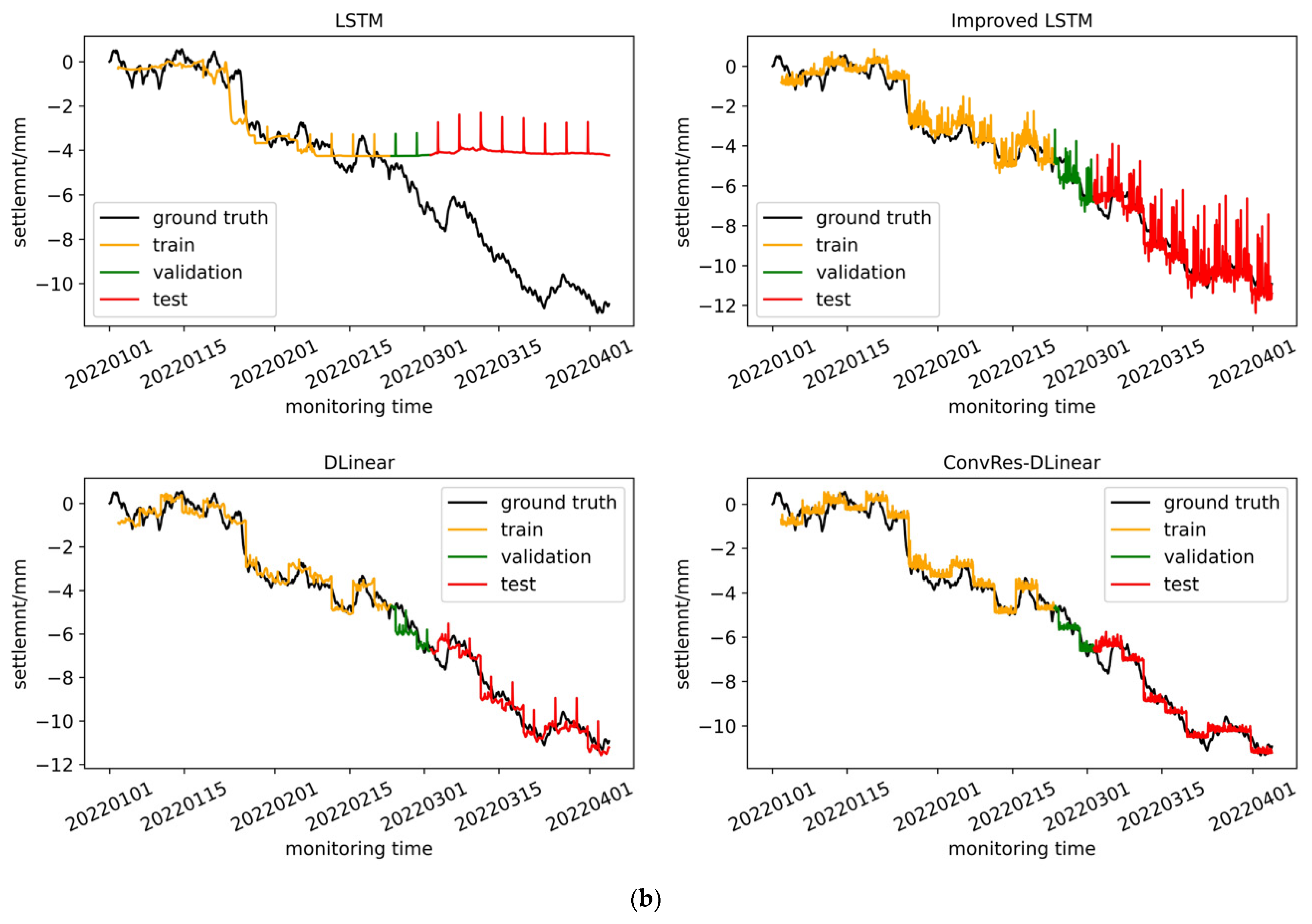
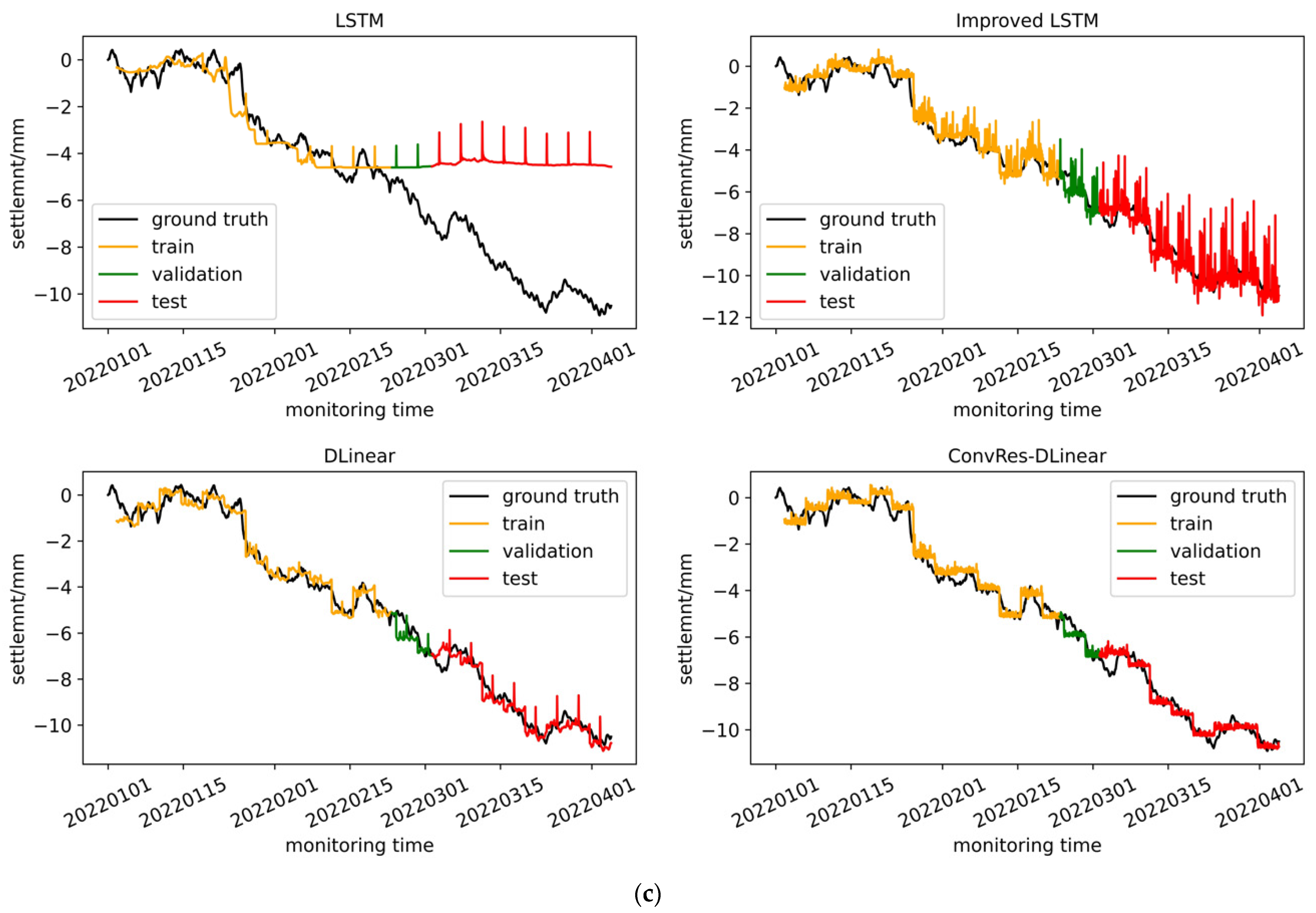
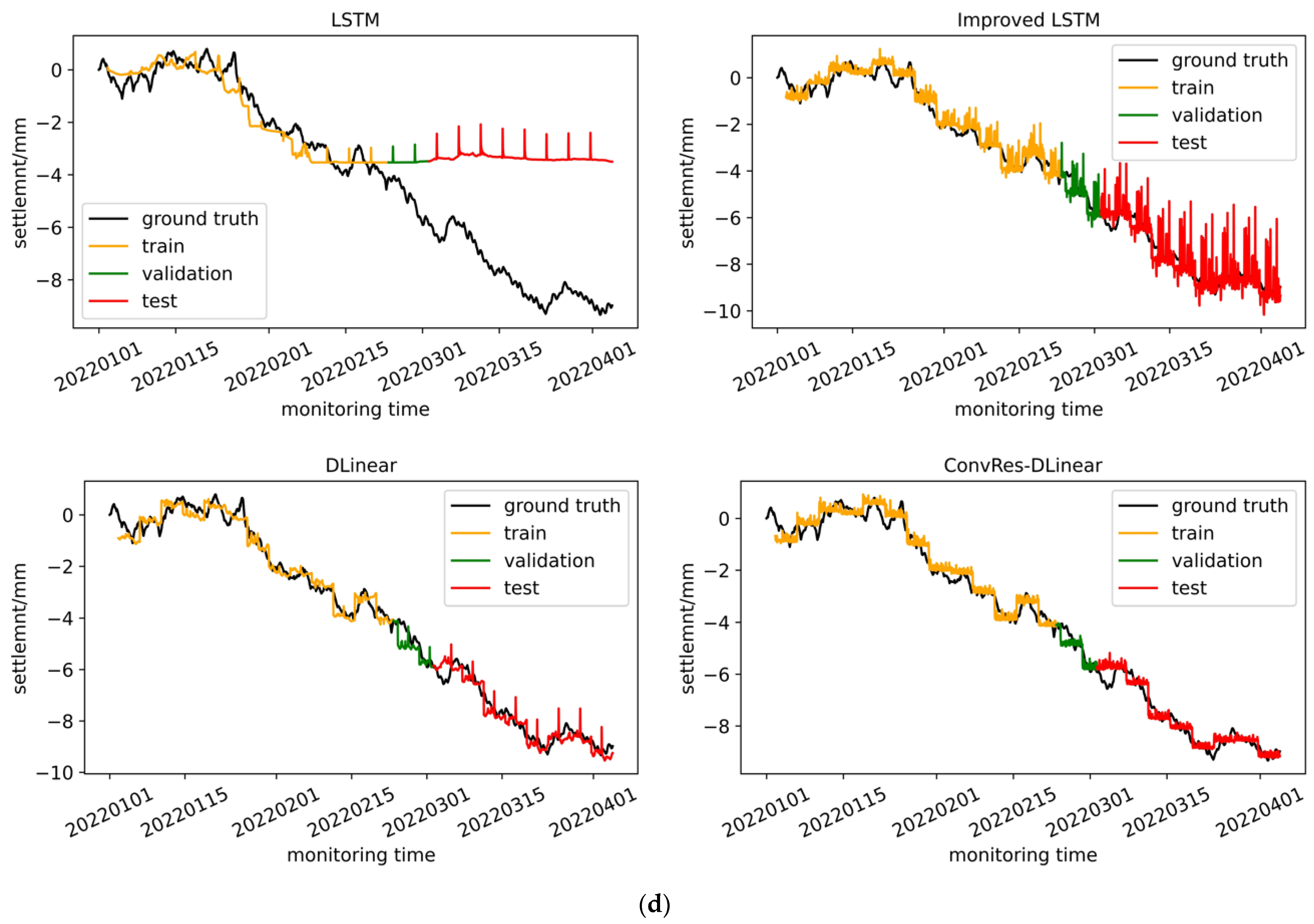
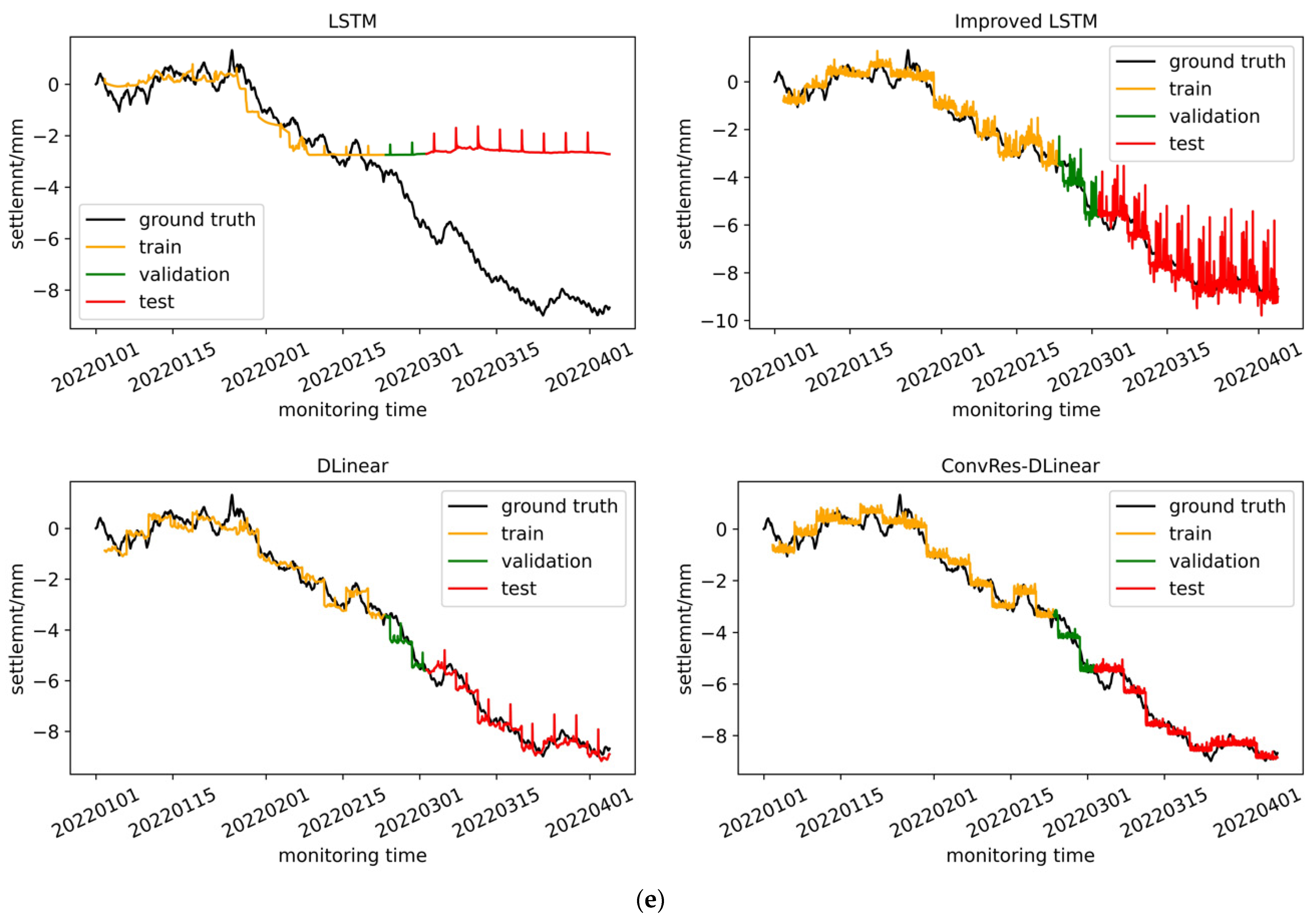
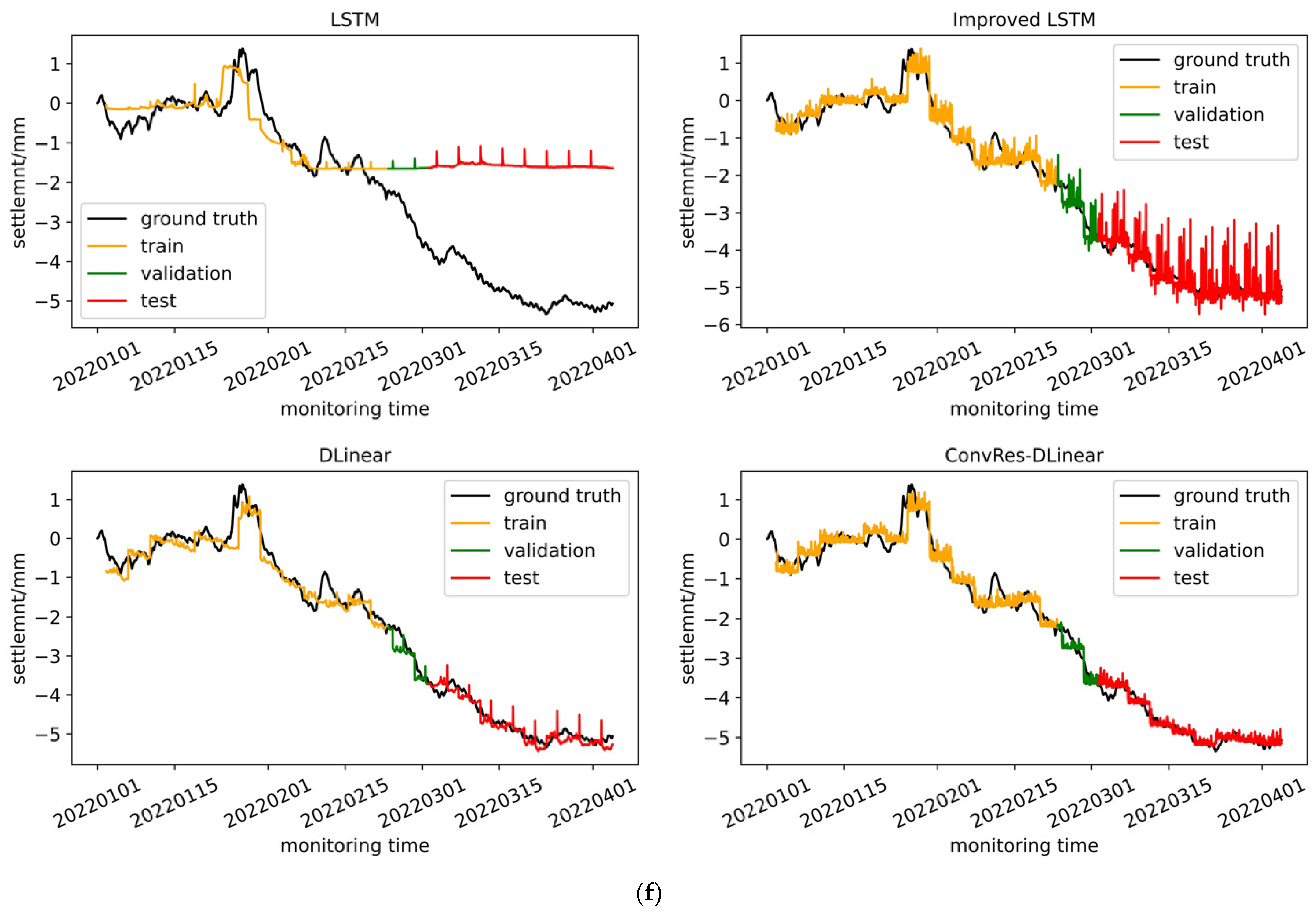
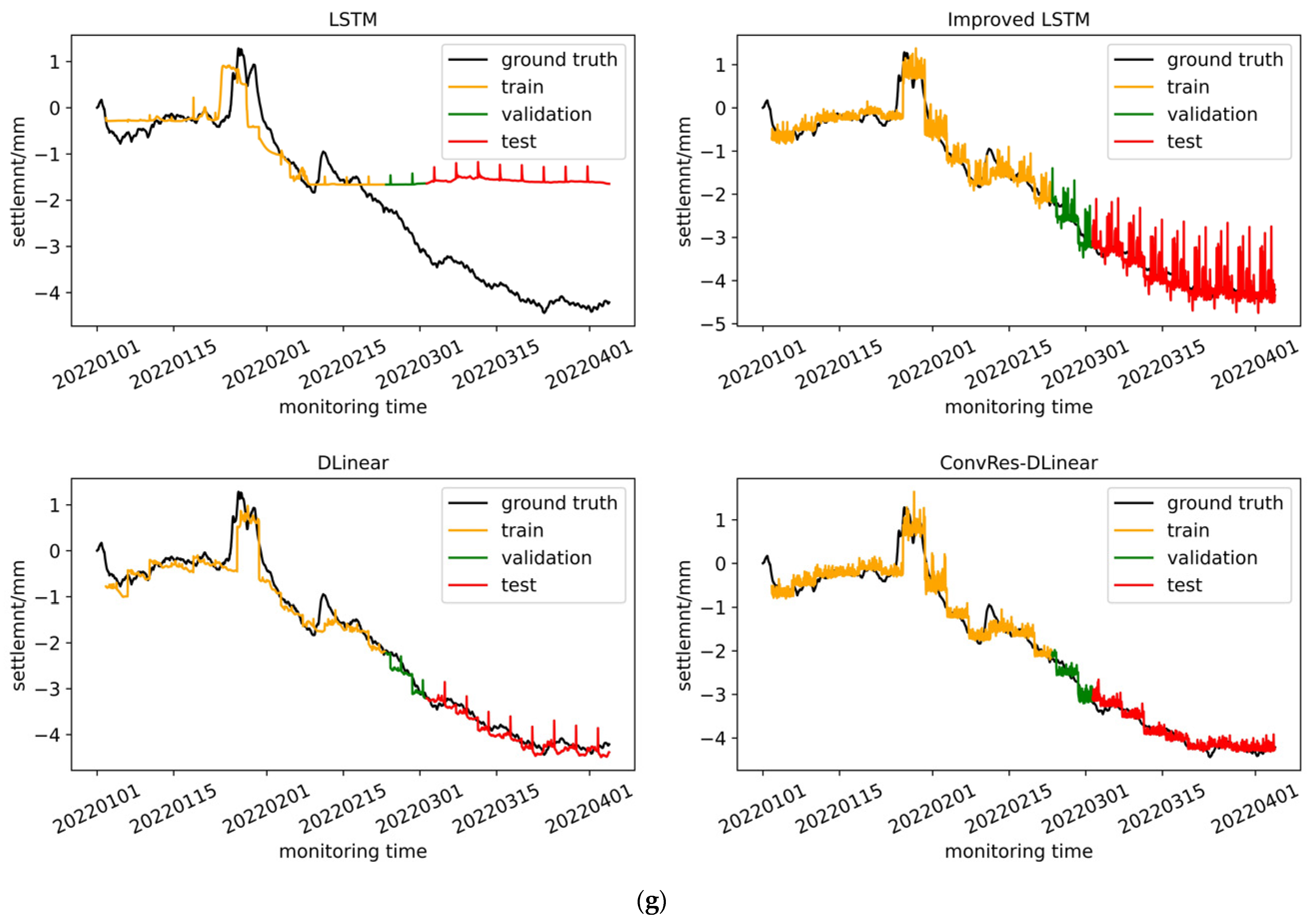
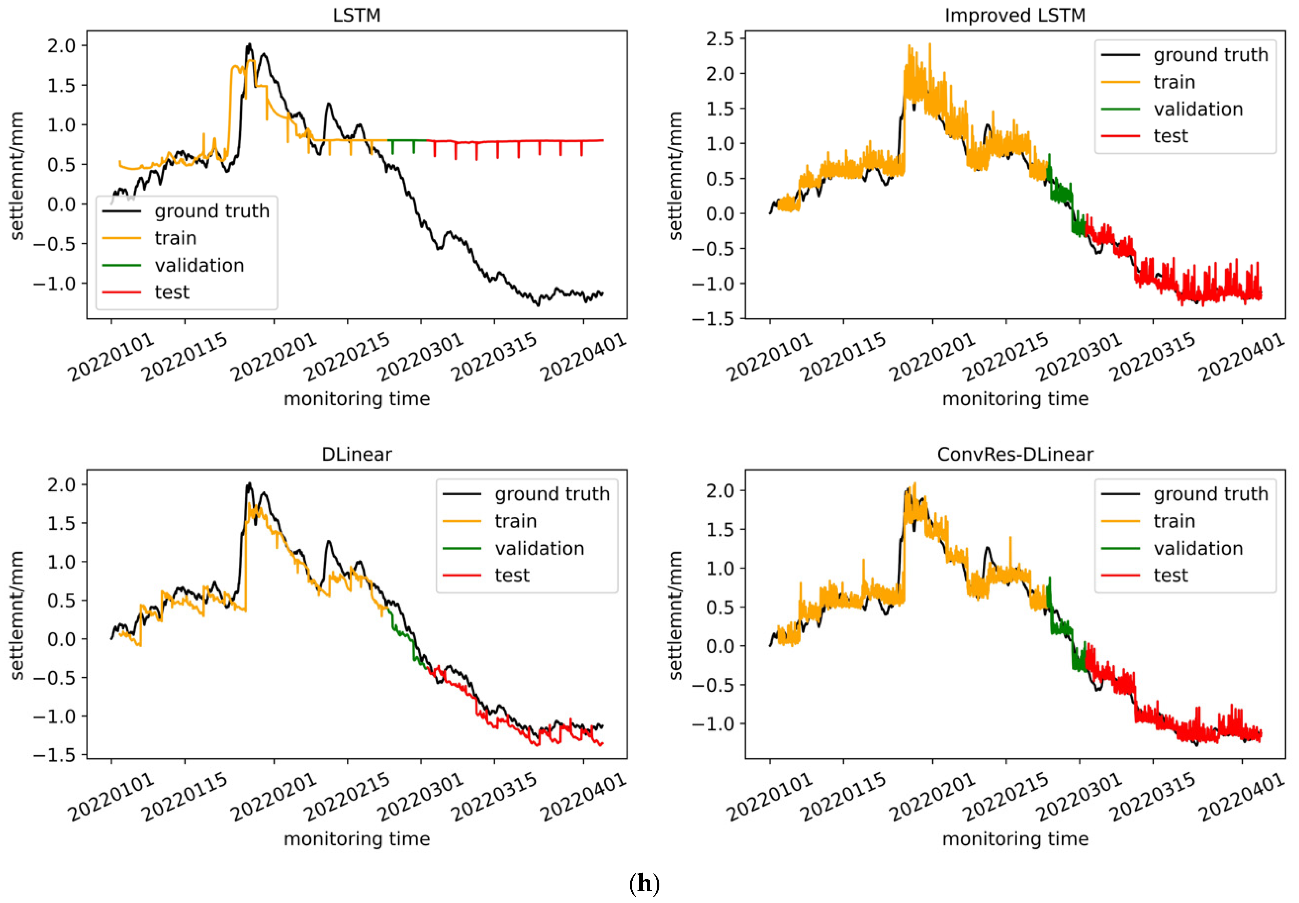
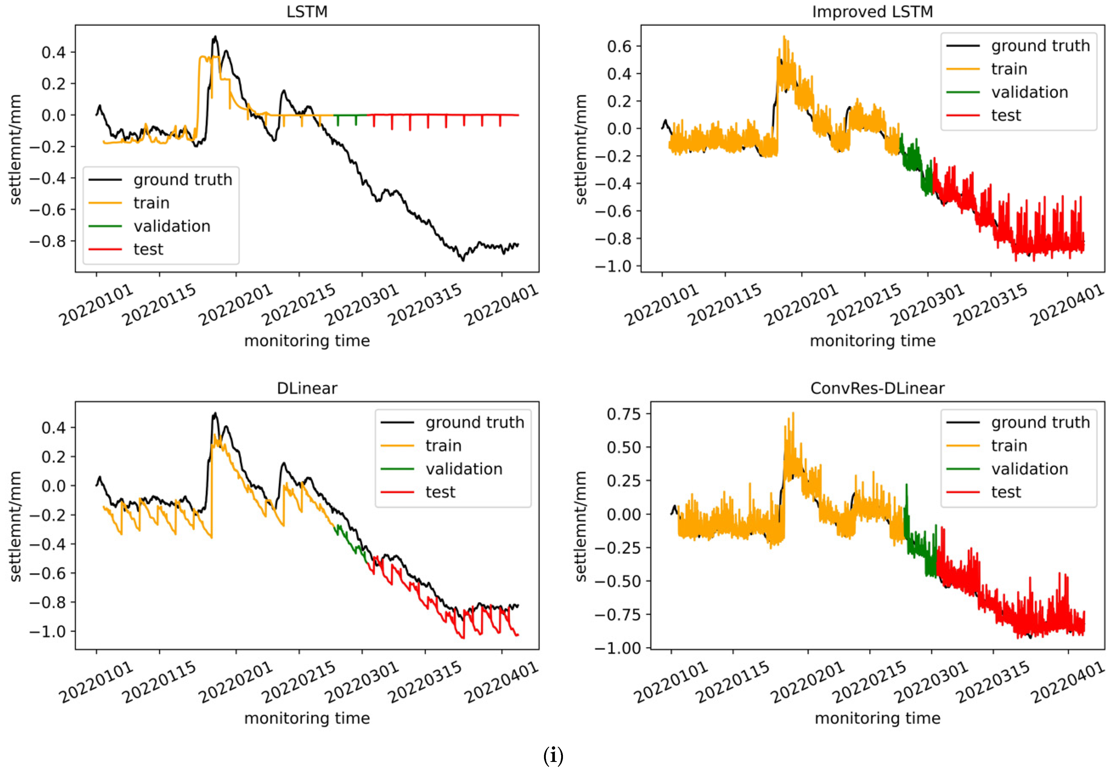
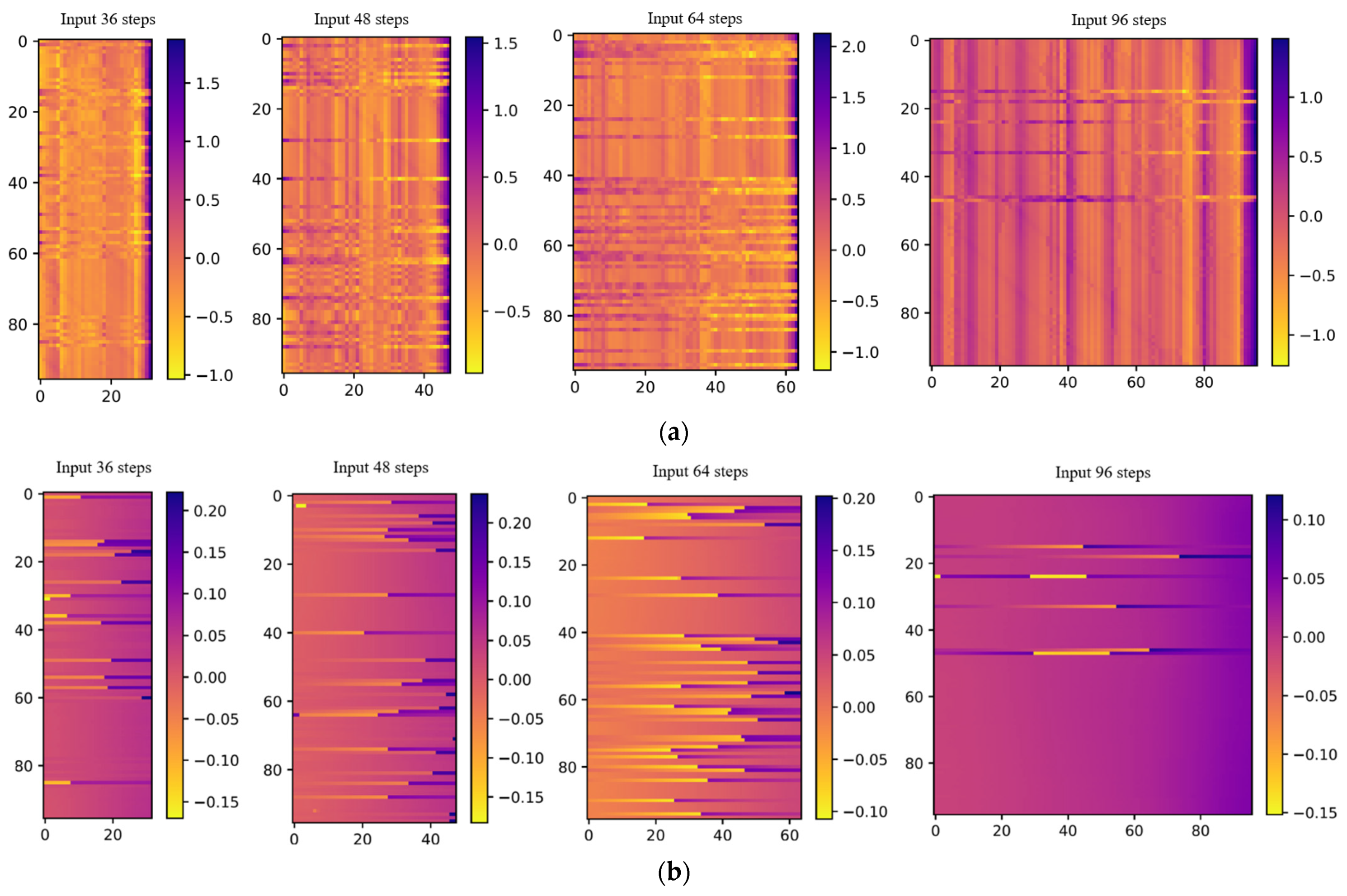
We trained the four models described in Section 2, namely LSTM, improved LSTM, DLinear, and ConvRes-DLinear, using the structural deformation monitoring time series dataset constructed in Section 4, and compared their effects. Furthermore, we attempted to visualize the correlation between the inputs and labels of the time series prediction at the weight level, aiming to interpret it. From the comparison below, it can be seen that the DLinear architecture model has simplicity and effectiveness in time series prediction, and our ConvRes-DLinear has more accurate prediction.

The different hyper parameters for each model are presented in

Table 1. Hyper parameters for LSTM, improved LSTM, DLinear and ConvRes-DLinear.

Model Name	Num_Layers	Conv1d/Pool Kernel Size	Validation Data RMSE/mm	Test Data RMSE/mm
LSTM	2	\	0.72	3.21
Improved LSTM	2	\	0.64	0.72
DLinear	\	25	0.53	0.65
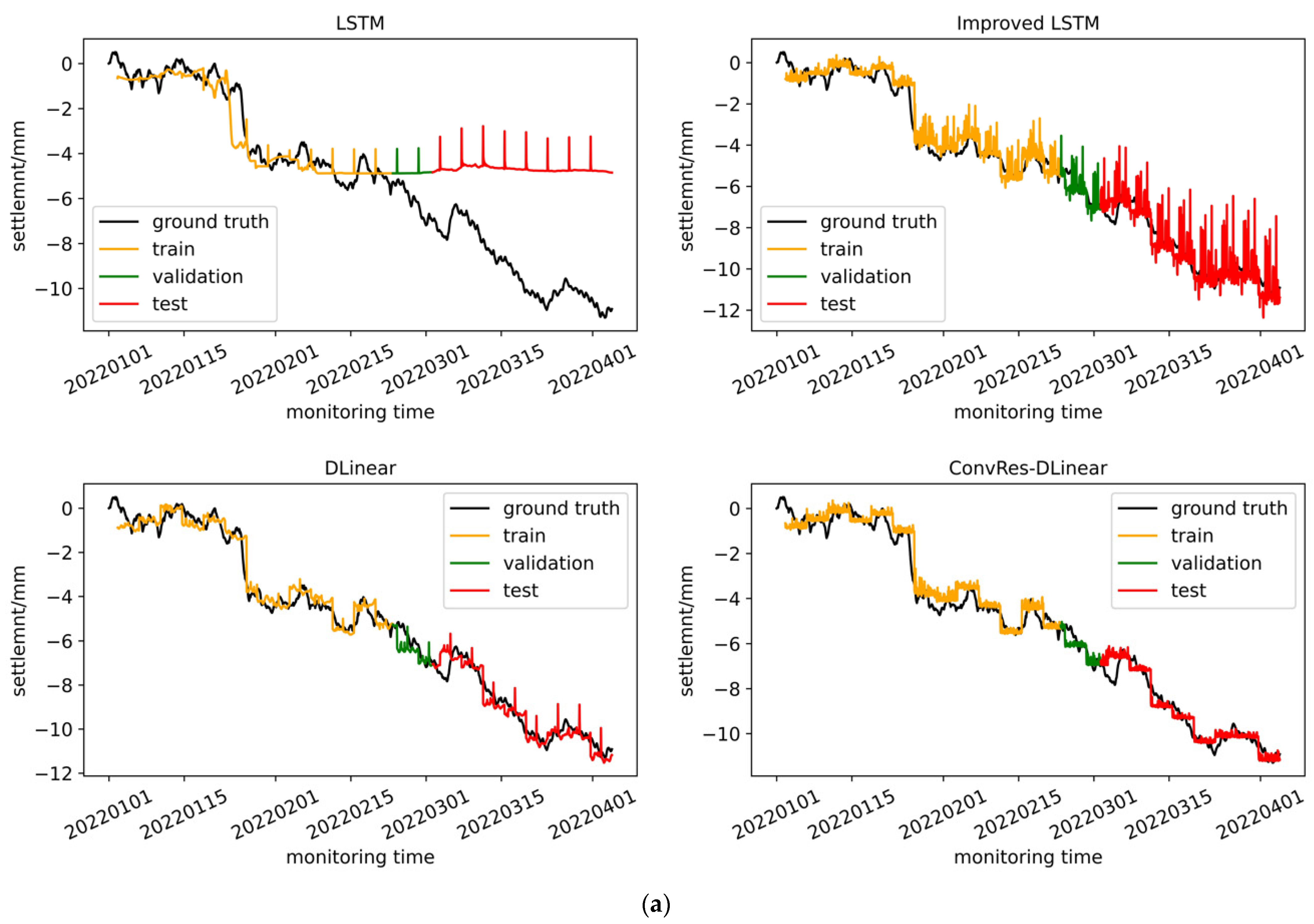
ConvRes-DLinear	\	25	0.52	0.55

, with all of these parameters having undergone grid search to select the optimal values. The time step is set to 96, and the prediction step is also 96, meaning that the model uses data from the previous four days to predict data for the following four days. Since our monitoring device records data every hour, the model’s task can be described as predicting data from the next 96 monitoring points using data from the previous 96 monitoring points. If the model’s prediction accuracy is high enough, it can be deployed on the monitoring platform for subway operations and maintenance, enabling operators to have a four-day lead time to decide whether to repair the tunnel. This will be a practical engineering reference. The model training was carried out on hardware consisting of an Ubuntu 22.04LTS system and an NVIDIA RTX3050 4G GPU, using AdamW optimization and early stopping strategy with patience equal to 5. The dataset was divided into training, validation, and testing sets at a ratio of 5:1:4. Finally, the performance of each model on the training, testing, and validation sets is shown in Figure 9.

6. Results

The prediction results of LSTM, improved LSTM, original DLinear and ConvRes-DLinear can be seen in Figure 9 and Table 1. Based on the RMSE value, ConvRes-DLinear performed the best among all models, followed by DLinear, and then by both LSTM models. From the performance comparison in Figure 9, ConvRes-DLinear showed higher volatility than DLinear but converged better to each segment’s peak value. The stronger fitting ability to the peak value may come from the convolutional layer replacing the pooling layer and incorporating the input geological information into our longitudinal settlement monitoring time-series data. In contrast, compared with traditional RNNs such as LSTM used in this paper, its predictive performance was not satisfactory. On the validation and test sets, LSTM’s predicted values were close to a constant value, with almost no fluctuation. For long-range prediction tasks, LSTM displayed weakness in fitting time-series changes with different hidden variables and shared weight matrices at each time step. On the other hand, the improved LSTM, based on the idea of residual path, could capture the trend of the tunnel longitudinal settlement but showed very high volatility in both validation and test sets, deviating significantly from the actual values. The improved LSTM’s grasp of the trend in time-series data came from the setting of a basic value in the residual block, which was set as the last time step’s deformation in the input sequence. Under the premise of no unexpected events causing mutations, the settlement deformation in the predicted time interval did indeed continue based on the last time point in the historical period. This is also why the improved LSTM could fit the general trends of the deformation.

7. Discussion

7.1. Model Comparison

Based on the accuracy comparison of four models in Figure 9 and Table 1, the superiority of the DLinear architecture in time series prediction is perfectly demonstrated, while the improved ConvRes-DLinear shows remarkable performance in fitting peaks. These models are simple, accurate, and capable of predicting long time steps, thus they will be deployed in the monitoring background of metro operation to show their significance in ensuring metro operation. However, despite the simple structure and superior performance of DLinear, its advantages are still a black box. We need to answer a core question: what did the model learn in time series datasets? This has been a confusing issue for researchers in the field of deep learning for many years [32]. For example, in the field of computer vision, there is GradCam [33] based on the principle of automatic differentiation, which is used to observe which part of the feature map plays a crucial role in the final output, and there are works visualizing the feature maps of various layers to qualitatively judge the mo’el’s learning on the dataset. In the field of NLP, researchers observe where the mo’el’s analysis of world knowledge and grammatical lexicon is distributed through ablation experiments. In conclusion, although deep learning relies on powerful computing power and massive parameters to perform specific prediction tasks, the actual distribution of parameter learning is still a black box. Therefore, we need to understand the mechanism of model learning qualitatively through some means. Only by grasping the model learning mechanism qualitatively, can we better design different model architectures for specific tasks or more general architectures for multiple tasks.

7.2. Model Explainability

In our prediction task on the subway longitudinal deformation time series dataset, it is critical to understand the correlation between historical and future data in the time series. This leads to another question, which is the optimal length of the historical data time window for improving the accuracy of the model prediction. Thanks to the succinct architecture of DLinear, we can directly analyze the time series correlation between input and output by visualizing two linear projection matrices. Meanwhile, we can also train multiple DLinear models with different lengths of historical data and observe the correlation on the time series sequence and prediction errors reflected by their projection matrices. Through these methods, we not only determine the best prediction time step for DLinear models on our subway longitudinal settlement prediction data set but also further explore the correlation between historical and future data. This correlation implies a lag effect of tunnel settlement, where the current environmental disturbances have a significant impact on the future that cannot be ignored. The analysis of this point helps us to establish the interaction between soil layers and tunnels in the current geographical environment. Although this is a simple conclusion, it is extremely useful in numerical simulation and helps to design excavation time steps to better simulate actual situations.

This paper analyzes the two linear projection matrices in the proposed ConvRes-DLinear, as shown in Figure 10. Since the data flow in ConvRes-DLinear is different from that in ordinary neural networks, we need to explain the specific meaning of the weight visualization in Figure 10. The input data undergoes one-dimensional convolution and exponential averaging, obtaining the regular x_seasonal and irregular x_trend parts of the variations, and then undergoes transpose once. After the transpose, the feature dimension, originally linear transformation of settlement of different segments, is transformed into the temporal dimension feature. Subsequently, the two transposed data x_seasonal^T and x_trend^T are respectively linearly mapped with the two weights we want to visualize, which are then superimposed before the prelu activation function. Therefore, each column of the weight parameter visualization actually corresponds to the data at a certain time point with respect to the historical data. We summarize the temporal correlation of the time series by observing the relative sizes of the columns. It can be seen that regardless of the length of the input time series, historical states closer to the future have a greater impact on the future, which is reflected in the two weight matrices of each time step. Moreover, the magnitudes of the two weight matrices at each time step are significantly different, because in our time series dataset, after exponential averaging, the magnitude of irregular data (trend) is larger than that of regular data (seasonal), and our model may learn two weight matrices with different magnitudes to balance the contribution of these two data parts to the final prediction, which is opposite to the data magnitude.

Moreover, as shown in Figure 11, the accuracy of the models constructed and trained at the various time steps between 36 to 96 also different. The RMSE error is the smallest when the time step is 73, so 73 is set as the final prediction step. This suggests that the originally set time step of 96 actually includes historical data that is too far away from the future state to have any effect on it. If our model still treats this part of the data as an independent variable and inputs it into the model, this will cause overfitting, and the additional historical data is not a feature in this case; it is an error. This causes the model to fail to converge to the global optimum. Additionally, if the time step is too small, the historical data that are related to the future state are not fully input into the model, causing the model to fail to learn the complete law of the historical state transitioning to the future state, which also leads to a decrease in prediction accuracy. Therefore, for high-precision prediction tasks, it is important to select a suitable time step by grid search or based on geological meaning.

8. Conclusions

This paper provides a summary of the current state-of-the-art in time series prediction and proposes an improved approach based on a new paradigm called the DLinear architecture, which is applied to the prediction of deformation in shield tunnels during operation with integration of environmental geological disturbance information. The proposed approach involves three key improvements:

(1)

We determine the starting time and calculate the increment for each time step of the input time series data. We then apply a residual block so that the starting time’s data is added to the model’s data stream before the PRelu activation function, which replaces standard data normalization.

(2)

Secondly, we incorporate geological information into the input as a bias, which can be customized when preparing the dataset and applicable to various deformity detection problems. We provide a specific methodology to define the bias based on construction process information, in which implicit modeling of environmental geological information was performed.

(3)

Lastly, we add a one-dimensional convolution before exponential averaging to fuse the input time series sequence differences and geological information, as the convolution’s parameters are learnable, it has greater parameter redundancy than one-dimensional pooling.

We obtain a large amount of continuous longitudinal deformation data from monitoring equipment VDMS and completed training of LSTM, improved LSTM, DLinear, and ConvRes-DLinear models based on the data from the Hangzhou Metro monitoring project. The results indicate that the proposed ConvRes-DLinear model outperforms LSTM in terms of prediction accuracy and can better fit the extreme values inside the time series data compared to the original DLinear model. The proposed ConvRes-DLinear model with integration of implicit geological information successfully captured the patterns of longitudinal settlement in the tunnel by fully utilizing prior information. Furthermore, we attempt to observe the correlation of shield tunnel deformation time series on time and distance using weight visualization based on the proposed ConvRes-DLinear model and determine the optimal time step for time series prediction. We find that there is a strong correlation between historical states close to future data and future state changes. If the historical time step input to the model is too long or too short, it will lead to a decrease in prediction accuracy. We suggest this is because distant data from future n-time step outputs will be regarded as errors, while a short time step input does not capture the implicit rules of learning from the past to predict the future.

Finally, our future work will focus on further improving the model architecture and exploring better methods to represent geological information like using meta-learning to search for better network layer architectures and more suitable weight initializations. Additionally, other representation methods can be explored to better capture the environmental perturbations of different deformity detection problems.