A Low-Cost, Repeatable Method for 3D Particle Analysis with SfM Photogrammetry

Abstract

The characterisation of particle shape is an important analysis in the field of sedimentary geology. At finer scales, it is key for understanding sediment transport while at coarser scales, such as boulders, it is vital for coastal protection. However, the accurate characterisation of particle shape is restricted by the application of 2D imaging for 3D objects or expensive and time-consuming 3D imaging methods such as X-ray tomography or laser scanning. This research outlines a low-cost, easy-to-use 3D particle imaging and shape characterisation methodology employing structure-from-motion (SfM) photogrammetry. A smartphone device was used to capture 2D images of pebble/cobble-sized samples, which were converted to 3D image models using SfM. The 3D image models were then analysed using a comprehensive set of 16 size and shape parameters. Furthermore, a minimum resolution, independent of particle size, is proposed here for the 3D image models for reliable and reproducible size and shape analysis. Thus, the methodology presented here for 3D particle imaging and size and shape analysis can be translated for a range of particle sizes. This work thus opens a pathway for the use of readily accessible imaging devices, such as smartphones, to flexibly obtain image data both in situ as well as in laboratories, thus providing an immensely powerful tool for research and teaching.

1. Introduction

Particle shape quantification is an important analysis carried out in a range of geological disciplines such as sedimentary geology [1], volcanology [2,3], geomorphology [4], structural geology [5], and petrology [6]. In sedimentary geology, shape quantification has been used as a tool to decipher the origin, transport, and deposition history of sedimentary particles. Examples of particle shape analysis applications in recent sedimentary research include discrimination of the sedimentary depositional environment [7,8,9,10,11], textural maturity analysis [11], bedload transport [12,13], Martian geology [14,15], bulk rock property [16,17], and provenance analysis of zircon grains [18].

The methodology for particle shape analysis has substantially evolved over one century [1,19,20]. Earlier attempts at shape quantification used a manual approach and were thus tedious and time consuming in nature (e.g., [21,22]). Visual comparison charts were introduced as a result to simplify the analysis [23,24]. However, shape characterisation based on visual charts suffers from user bias and reproducibility [25,26]. In the last two decades, there has been significant development in the field of automated quantitative shape analysis methodology [4,20,27,28,29,30,31].

Quantitative particle shape analysis is usually carried out in either 2D or 3D [1,19,20]. Methods of 2D shape analysis require optimal imaging based on particle size (e.g., digital cameras for gravel, digital microscopes for sand, and SEM for silt/clay/sand fractions). On the other hand, laser scanning and X-ray computed tomography have been frequently used for 3D imaging of particles in engineering disciplines (e.g., [32,33,34,35]). Three-dimensional imaging of particles provides several pieces of additional physical information regarding morphology (and material properties in the case of X-ray tomography). However, laser scanning and X-ray tomography techniques have been rarely used in sedimentary research, possibly due to costly and time-consuming methods of image acquisition and processing. Therefore, most of the recent geoscience research either uses 2D shape analysis [9,11,18,36,37,38,39] or proposes techniques for 2D shape analysis [3,4,31,40,41,42]. An alternative methodology that can be used for obtaining 3D data is photogrammetry.

Photogrammetry is the process of making direct measurements from photographic data. Structure-from-motion (SfM) is a particular branch of photogrammetry that, like stereoscopic photogrammetry, allows the 3D structure of objects of interest to be resolved/reconstructed through a series of overlapping but offset images [43]. Given the low cost and user-friendliness of the method in commercially available software, SfM photogrammetry has recently gained considerable interest. The method relies largely on the scale-invariant feature transform (SIFT) algorithm [44] which allows features in overlapping but offset images to be detected. The method has been successfully applied in terrestrial geomorphology as well as in deep marine environments owing to the repeatability of the method [45,46,47,48]. Moreover, when SfM is applied systematically as in archaeological studies with >60% image overlap (e.g., [49,50,51]), remarkably detailed 3D reconstructions can be generated.

Due to a dearth of studies in sedimentary geology adopting photogrammetry-based 3D particle analysis methodology, wider practical applications (e.g., sedimentary fabric analysis) remain elusive. Researchers in engineering disciplines have made some progress in this direction (e.g., [35,52]). However, there is still a lack of studies applying 3D photogrammetry to sedimentary particles for obtaining sedimentary geology-oriented 3D shape analysis. Furthermore, there is currently a lack of research directed towards the minimum resolution required for 3D shape and size characterisation. This work aims to introduce a 3D photogrammetry and particle shape analysis methodology. In this context, the objectives of this research are to:

• Present a cheap, fast, and reproducible methodology for obtaining high-quality 3D particle data using SfM-photogrammetry;
• Characterise sedimentary particle shape and size using the obtained 3D photogrammetry data;
• Determine the minimum resolution required for 3D shape and size characterisation.

The next section describes the samples used in this study followed by details of the methodology. The workflow for 3D imaging presented here facilitates a cheap and readily accessible technique that can be utilised flexibly by users.

2. Materials and Methods

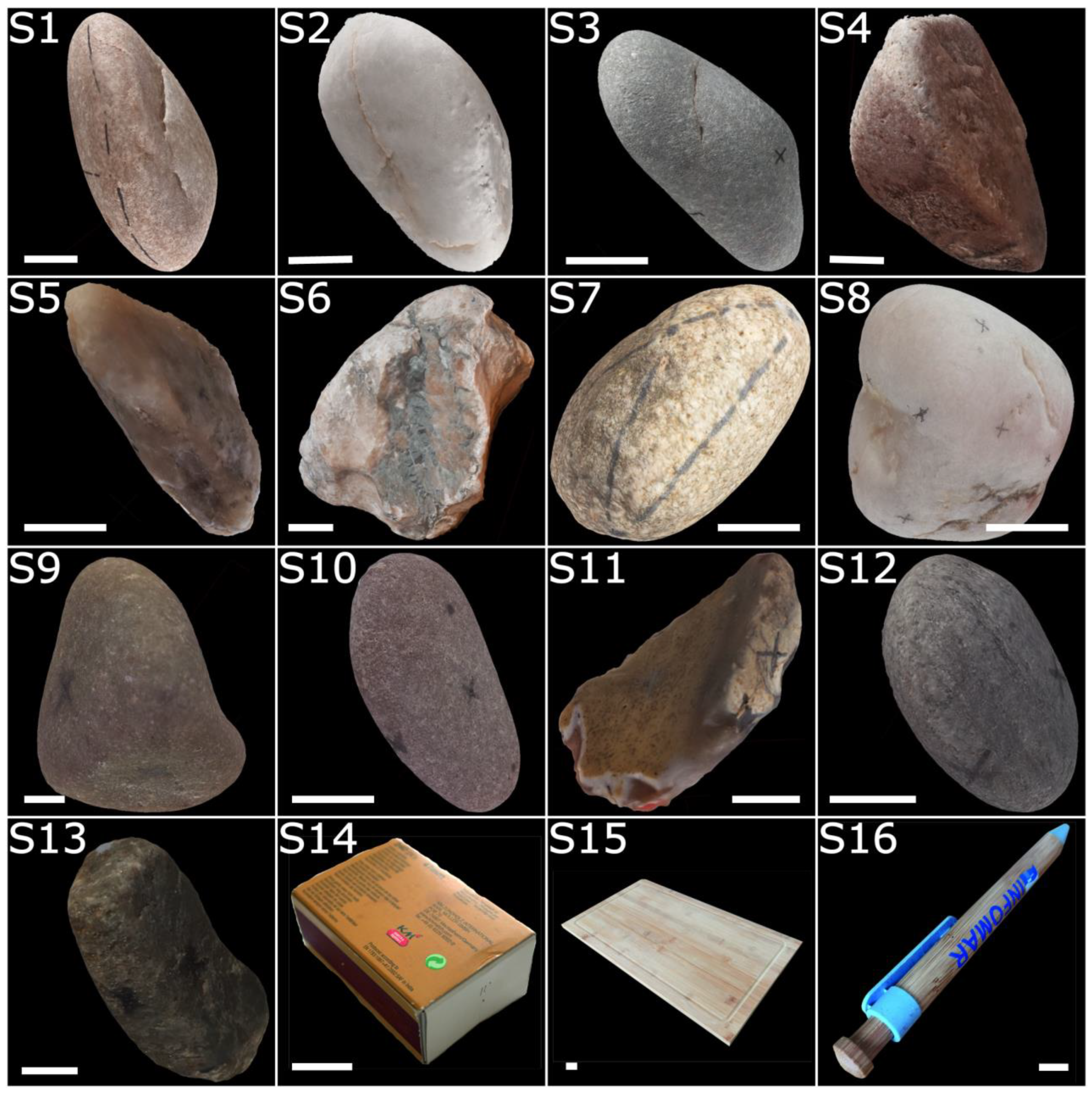
This study utilises sedimentary particles as well as the man-made reference samples described below (Section 2.1). The methodology used to analyse the samples includes SfM photogrammetry (Section 2.2), particle shape and size analysis (Section 2.3), and determination of minimum required image resolution (Section 2.4).

2.1. Samples Used

In this study, we used a total of 16 sample objects consisting of 13 clasts (S1–S13) from the beach environment and 3 reference materials (S14–S16, see Figure 1). The beach samples were collected from Cushendun Beach, Co. Antrim, Northern Ireland (55°7′54″ N, 06°2′26″ W). The clasts consisted of micro-granite and schist from the Dalradian supergroup [53]. The pebble/cobble-sized clasts were selected to provide as much natural variation in sedimentary particle shape as possible.

Additionally, the following three reference materials were used in this study: (1) S14—a match box, (2) S15—a chopping board, and (3) S16—a pen. The three reference materials: S14, S15, and S16 provide an analogue for cuboid, platy, and rod shapes, respectively. Next, SfM photogrammetry of the samples is described.

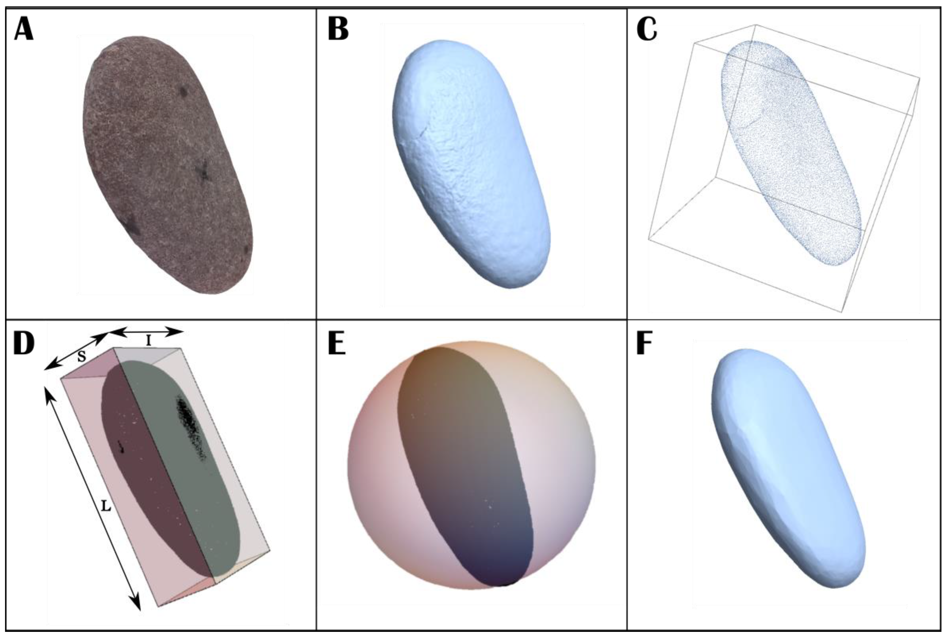
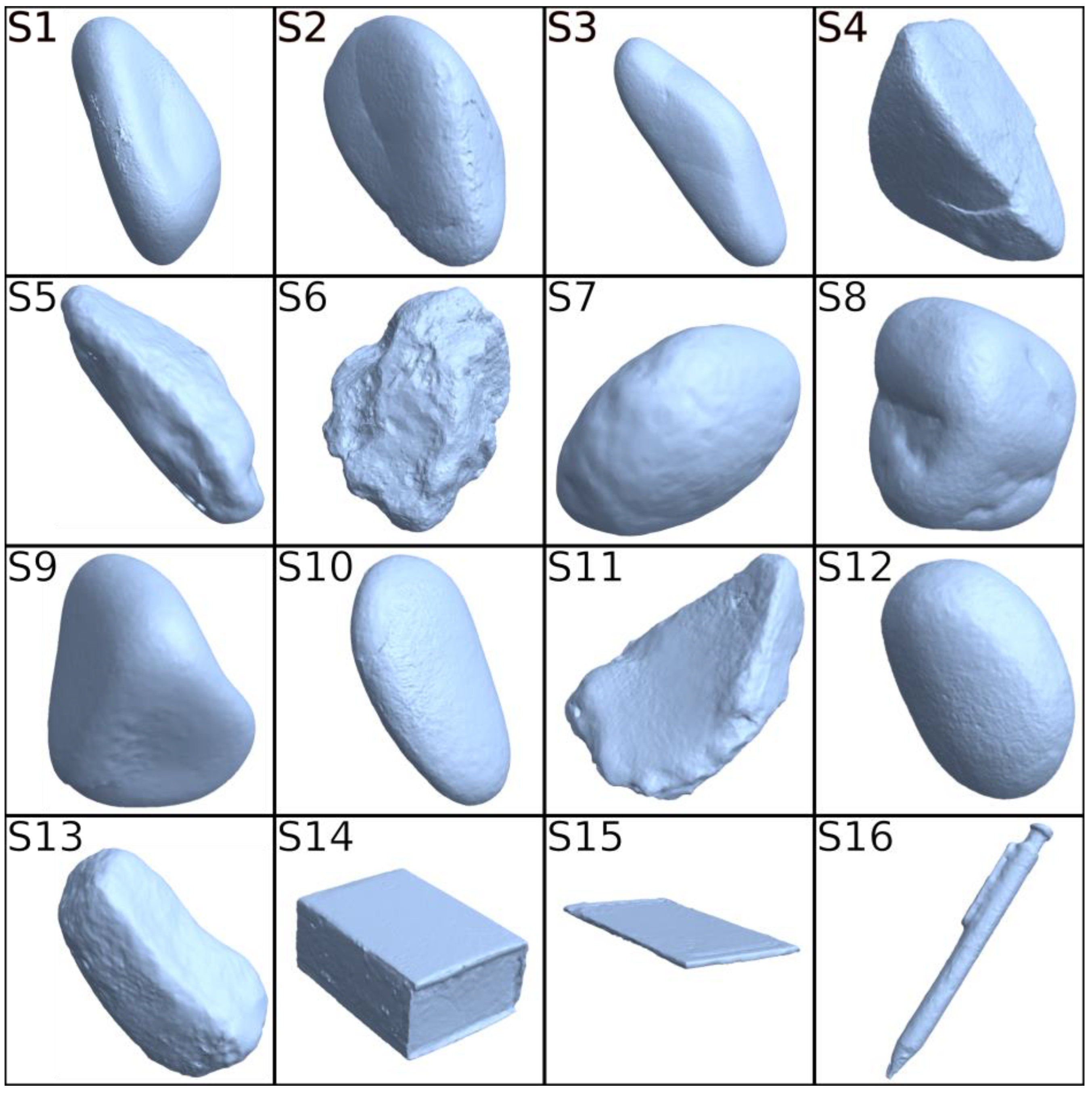
2.2. Structure from Motion Photogrammetry

A systematic SfM method was applied to a series of clasts and common household objects. The systematic method utilised herein can be divided into three steps: survey set-up, image acquisition, and data processing. For the survey set-up, all objects are placed on a homogenously lit-up stage. The stage is approx. 30 cm × 30 cm. To achieve homogenous lighting across the stage, four lighting sources were placed approx. 90 degrees from each other, centred around the stage, and utilised. The stage was then subsequently marked with four points ($a, b, c, \mathrm{and} d$). The distance between each point was measured for the purpose of scaling the model during processing.

Given that the full surface of the model is required to be reconstructed, the object is imaged in two overlapping segments (Figure 2). Accordingly, for the image acquisition step, the object of interest was secured to the centre of the stage with modelling putty. The object was aligned with its longest axis ($L$) aligned vertically. Images were acquired approx. every 10 degrees (minimum) around the centre of the object. The camera was pointed obliquely towards the centre of the object for each image acquired. Each image also included the full stage where points $a$ to $d$ were included. A minimum of three of these points were visible in all images. The camera utilised during acquisition was from a Huawei P30 Pro which has three main lenses. The specifications of the lens utilised for this research are 40 MP, f/1.6, 27 mm. The images were acquired as *.raw which were subsequently converted to *.jpeg. Once completed, the object was removed from the stage and the model was turned ‘upside-down’ where the process was repeated resulting in two sets of image data for each ‘side’ of the object. This was to ensure that image data from the full surface of the object were acquired. Image position did not appear to have a considerable impact on the final point cloud. However, a systematic image acquisition survey was followed to ensure consistency in the results.

All data were imported to Agisoft Metashape (www.agisoft.com (accessed on 4 May 2023)). Each of the two image sets from the model was imported separately (referred to as ‘chunks’ in Agisoft) to the same project. The process of image alignment was completed separately for each chunk. The settings utilised were ‘highest’ for accuracy, generic preselection, a key point limit of 20,000, and a tie point limit of 2000. When creating dense clouds, the ‘Ultra high’ quality was chosen for each. Clear, obvious features on the surfaces of the object such as cracks, fractures, mineral grains, and colour changes were identified and manually highlighted by adding point markers in Agisoft on the object from both image sets. The two image sets were subsequently automatically merged using the Align Chunks tool based on the identified markers. This essentially stitches both sets of images together using the known position of common features that were manually added. Once merged, points $a$ to $d$ were then used to scale the reconstruction. Subsequently, the stages and surrounding artefacts within the models could be removed via manual selection or selection and removal based on pixel colour, similar to the process utilised by [46,54,55]. A final dense cloud reconstruction was generated of the completed model and the resultant triangular mesh file was exported as a standard *.obj file format. This mesh model (from *.obj file) will be subsequently referred to as a “3D model” in this paper. The SfM photogrammetry process was repeated for each sample. The 3D models can be alternatively exported in *.xyz file formats or a range of GIS-friendly file formats based on user preference.

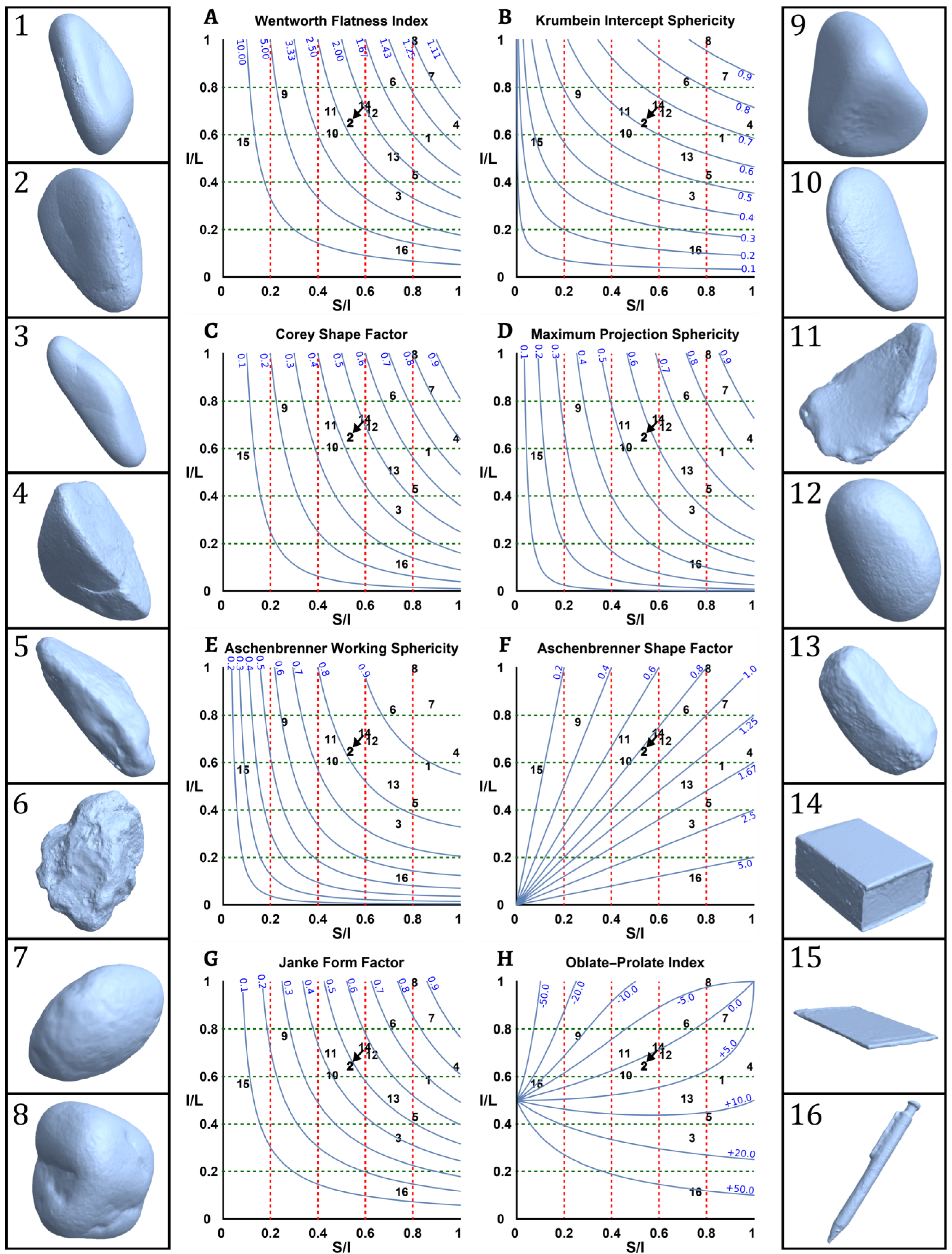
2.3. Shape and Size Parameters

A 3D model when referenced to physical dimensions can be used for calculating the actual size of the sample. Otherwise, the calculated length measurements will be in voxel units which would be devoid of physical sense. To give an example, a digital 3D cube of 10 voxel units in length on each side can represent a physical cube of any size—50 mm or 50 cm, or even 50 km unit length. In this study, all the 3D models are referenced to physical dimensions and scaled to metre units. A Mathematica (https://www.wolfram.com/mathematica/ (accessed on 4 May 2023)) script was developed by the authors to calculate the size and shape parameters (See Supplementary Data: File S1). A total of 16 commonly used sedimentary size and shape parameters described in

Table 1. Size and shape parameters used in this study.

	Parameter	Formula	Range	Remarks/Reference
	Size
1	Long Axis	$L$	0 to ∞	The three axes of the particle are measured as the length of the three sides of the best-fit-oriented cuboid over the particle [1]
	Intermediate Axis	$I$	0 to $L$
	Short Axis	$S$	0 to $I$
	Shape
2	Flatness (F)	$\frac{S}{I}$	0 to 1	[1]
3	Elongation (E)	$\frac{I}{L}$	0 to 1	[1]
4	Wentworth Flatness Index (WFI)	$\frac{L + I}{2S}$	1 to ∞	[56]
5	Krumbein Intercept Sphericity (KIS)	$\sqrt[3]{\frac{IS}{L^2}}$	0 to 1	[23,57]
6	Corey Shape Factor (CSF)	$\frac{S}{\sqrt{LI}}$	0 to 1	[58]
7	Maximum Projection Sphericity (MPS)	$\sqrt[3]{\frac{S^2}{LI}}$	0 to 1	[59,60]
8	Aschenbrenner Working Sphericity (AWS)	$\frac{12.8\sqrt[3]{F^{2}E}}{1 + F\left(1 + E\right) + 6\sqrt{1 + F^2(1 + E^2)}}$	0 to 1	$F$ is $S/I$ and $E$ is $I/L$ [61]
9	Aschenbrenner Shape Factor (ASF)	$\frac{LS}{I^2}$	0 to ∞	[61]
10	Janke Form Factor (JFF)	$\frac{S}{\sqrt{\frac{L^2 + I^2 + S^2}{3}}}$	0 to 1	[62]
11	Oblate–Prolate Index (OPI)	$\frac{10\left(\frac{L - I}{L - S} - 0.5\right)}{S/L}$	−∞ to +∞	[63]
12	Solidity (SOL)	$\frac{V}{V_{CH}}$	0 to 1	$V$ is the particle volume, and $V_{CH}$ is the volume of the convex hull [64]
13	Circularity (CIR)	$\frac{6V}{\sqrt{A{r}^3/\pi }}$	0 to 1	The ratio of particle volume $V$ to the volume of the sphere with an equivalent surface area to the particle $Ar$ [61]
14	Volume Sphericity (VSP)	$\frac{V}{V_{Cir}}$	0 to 1	$V$ is the particle volume and $V_{Cir}$ is the volume of the smallest circumscribing sphere to the particle [65]
15	Diameter Sphericity (DSP)	$\frac{D_V}{D_{Cir}}$	0 to 1	$D_V$ is the diameter of the sphere with equivalent volume to the particle, and $D_{Cir}$ is the diameter of the smallest circumscribing sphere [66]
16	Surface Area Sphericity (SAS)	$\frac{A{r}_v}{Ar}$	0 to 1	$A{r}_v$ is the surface area of the sphere with equivalent volume to the particle, and $Ar$ is the surface area of the particle [67]

were implemented in this study.

There are various methods of calculating particle size in 3D [1]. In this paper, a minimum volume cuboid (see Figure 3D) is fitted over a particle. The fitted cuboid’s length, width, and height are calculated as the size of particle’s three axes ($L$, $I$ and $S,$ respectively—Table 1 (1)). It is to be noted that the cuboid is oriented along the particle as opposed to being oriented along the Cartesian axes. In this study, the best-fit cuboid was computed using the in-built Mathematica function BoundingRegion (with MinOrientedCuboid option).

Altogether 15 shape parameters are used in this study (Table 1 (2 to 16)). A subset of the shape parameters (Table 1 (2 to 11)) can be calculated using the particle’s three axes ($L, I, \mathrm{and} S$). These shape parameters are flatness ($F$), elongation ($E$), Wentworth flatness index ($WFI$), Krumbein intercept sphericity ($KIS$), Corey shape factor ($CSF$), maximum projection sphericity ($MPS$), Aschenbrenner working sphericity ($AWS$), Aschenbrenner shape factor ($ASF$), Janke form factor ($JFF$), and the oblate–prolate index ($OPI$). These 10 shape parameters were compared with each other in a review study by [1].

Additionally, five commonly used shape parameters: solidity ($SOL$), circularity ($CIR$), volume sphericity ($VSP$), diameter sphericity ($DSP$), and surface area sphericity ($SAS$) were implemented in this study (see Table 1 (12 to 16)). The following geometrical measurements were required to compute the abovementioned shape parameters: particle volume, particle surface area, convex hull over the particle, and the smallest circumscribing sphere over the particle. The volume of the particle from its mesh was calculated by integrating the volume of each tetrahedron formed by joining the individual mesh triangles with the origin [68]. On the other hand, particle surface area, minimum bounding sphere, and convex hull were computed using the in-built Mathematica functions RegionMeasure, BoundingRegion (with MinBall option), and ConvexHullMesh, respectively.

Figure 3 shows a particle (S10, Figure 1) with its resultant 3D model, 3D point cloud, best-fit-oriented cuboid, smallest bounding sphere, and 3D convex hull. The shape and size parameters implemented in the Mathematica script were tested using a simulated cube (See Supplementary Data: File S2).

2.4. Minimum Resolution

Any particle image, whether in 2D or 3D, must have a sufficient image resolution to reliably carry out size and shape analysis [3,42,69,70]. Therefore, a minimum image resolution ought to be determined for the 3D imaging methodology discussed here. The readers are reminded that a 3D image can represent a physical particle of any given size. Hence, scaling of image resolution is necessary to compare the 3D image resolution of particles of varying physical sizes. In this study, the scaled resolution ($SR$) of a particle’s 3D image is defined here as:

$$SR=N_p/S{A}_n$$

(1)

where ${\mathit{N}}_{\mathit{p}}$ is the number of unique points in the particle’s 3D point cloud. In Mathematica, the 3D point cloud is generated using the vertices of the triangular mesh of the 3D model. $\mathit{S}{\mathit{A}}_{\mathit{n}}$ is the normalised surface area of the particle. The normalised surface area is defined here as:

$$S{A}_n=SA/L^2$$

(2)

where $\mathit{S}\mathit{A}$ is the particle surface area and L is the longest axis of the particle. Since $\mathit{S}{\mathit{A}}_{\mathit{n}}$ is the normalised surface area, it is dimensionless. Hence, the $\mathit{S}\mathit{R}$ is measured in point units. The normalisation of surface area with respect to the particle size ($\mathit{L}$) ensures that 3D image resolutions of particles with varying physical size are comparable. In its 2D analogue, calliper length has been successfully used earlier to normalise particle size [42]. 3D models of three samples (sample S8, sample S10 and sample S14) were imported to CloudCompare (https://www.danielgm.net/cc/ (accessed on 4 May 2023)), a piece of open-source point cloud and mesh data processing software. Here, models were resampled to varying scaled resolution and exported to analyse for variation in resultant shape parameter values. This study determines the minimal scaled resolution required for a 3D model to perform reproducible 3D particle shape analyses. The results of the above-discussed methodologies are presented along with a discussion in the next section.

3. Results

The samples shown in Figure 1 were imaged following the methodology described in Section 2.2. The resultant 3D models for the corresponding 16 samples are presented in Figure 4. The 3D models were created with scaled resolution of greater than 4800 points in each model.

The 3D image models were imported into Mathematica (as *.obj files) to compute the size and shape parameters (Table 1). Since the 3D models were scaled to physical dimensions in meters, it was possible to measure the physical size of the samples. The long axis ($L$) of the samples vary from 5.31 cm (S14) to 51.6 cm (S15), the intermediate axis ($I$) is in the range 1.62 cm (S16) to 29.36 cm (S15) and the short axis ($S$) varies within 1.22 cm (S16) to 9.62 cm (S8) range.

With the three axes calculated, the axis ratios result in particle shape parameters—flatness ($S/I$) and elongation ($I/L$). Lower values of flatness and elongation indicate flatter and more elongated sample respectively, and vice versa. Sample 15 (chopping board) depicted the lowest flatness value of 0.08, whereas the highest flatness value of 0.98 was displayed by sample 4. In case of elongation, sample 16 (pen) shows the lowest value of 0.11, whereas sample 8 depicts the highest elongation value of 0.99. The distribution of all the 16 samples on a flatness ($S/I$) versus elongation ($I/L$) bivariate plot is presented as Zingg’s diagram [71] in Figure 5. The shape parameters which rely on the particle size dimensions ($S,I,L$) can be displayed on the Zingg’s diagram [1]. Thus, in Figure 5, the curves of the following shape parameters are plotted on the Zingg’s diagrams to represent the sample shape variation: Wentworth flatness index ($WFI$), Krumbein intercept sphericity ($KIS$), Corey shape factor ($CSF$), maximum projection sphericity ($MPS$), Aschenbrenner working sphericity ($AWS$), Aschenbrenner shape factor ($ASF$), Janke form factor ($JFF$) and Oblate–Prolate index ($OPI$). The distribution of the sample values for the remaining five shape parameters—solidity ($SOL$), circularity ($CIR$), volume sphericity ($VSP$), diameter sphericity ($DSP$), and surface area sphericity ($SAS$) is displayed in Figure 6.

Figure 7 shows the values of the shape parameters (elongation, flatness, solidity, circularity, volume sphericity, diameter sphericity, and surface area sphericity) with respect to the variation in scaled resolution for sample 8, 10, and 14. There is a noticeable variation in the shape parameter values for the three samples below the scaled resolution of 2000 points, whereas the 3D image models above 2000 points display consistent shape parameter values. Therefore, a minimum resolution of 2000 points is recommended to be used when building 3D image models for shape analysis.

4. Discussion

4.1. Cheap, Fast, and User-Friendly Methodology

The methodology presented for 3D imaging in this paper is user-friendly as well as cost-effective. For example, the only costs incurred were fieldwork expenses (travel) and software. Images of many objects can be easily acquired using basic optical cameras, and given the availability of camera-bearing smartphones, image data can be captured with relative ease. Such image data, notably those from smartphones, are ordinarily geotagged with the smartphone GPS position while some smartphones even include local camera angle data. In this study, image data were acquired with a relatively common mobile phone camera. Post-processing of these image data with the SfM workflow can produce point clouds and full 3D models using several forms of software, including commercial (e.g., Agisoft Metashape and Pix 4D) and opensource (e.g., MicMap and VisualSFM) options. Readers interested in a comparison of the different approaches and/or software used for SfM photogrammetry are referred to [45]. Several computational tools and programming languages (e.g., Python, Octave, Matlab, and Mathematica) can be used to calculate the size and shape parameters from the 3D image models. In terms of time, the process of creating 3D models and analysing size and shape with the method utilised herein is relatively fast (<1 h each).

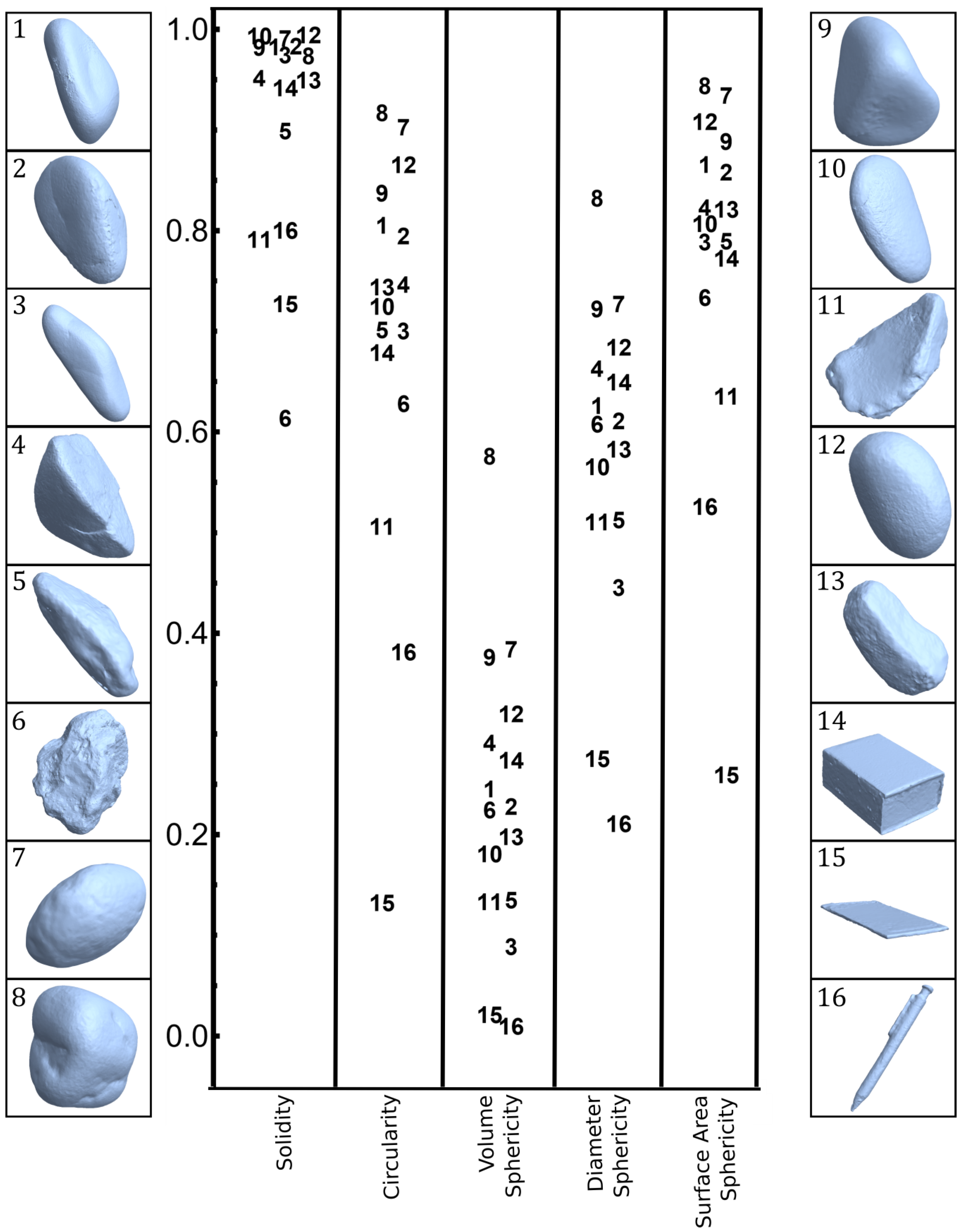
4.2. Particle Shape and Size Analysis

The sedimentary samples analysed in this study were selected to represent variation in naturally occurring clasts. This included angular- to rounded- and cylindrical- to spherical-shaped clasts. Furthermore, three reference samples (S14—a matchbox, S15—a chopping board, and S16—a pen) depicting cuboid-, platy-, and rod-shaped were used in the analysis. The SfM photogrammetry, shape, and size analysis methodology used in this study performs according to expectations. Sample S8, which is visually the most equidimensional and spherical clast, results in the highest value for Krumbein intercept sphericity, Aschenbrenner working sphericity, Janke form factor, circularity, volume sphericity, diameter sphericity, and surface area sphericity. On the other hand, samples S15 (platy-shaped) and S16 (rod-shaped) depict the lowest values for Krumbein intercept sphericity, Aschenbrenner-working sphericity, maximum projection sphericity, circularity, volume sphericity, diameter sphericity, and surface area sphericity. Using solidity parameters, a sample with indentations and rough corners (S6) can be distinguished from a sample with a smooth surface devoid of any indentation.

It is to be noted that differently shaped parameters display different ranges of values for the same sample set even though they represent sphericity and fall within the overall 0–1 theoretical range. For example, the sample values for volume sphericity lie within 0.01–0.58, whereas for surface area sphericity, they are 0.26–0.94 (see Figure 6). This is due to the definition of individual shape parameters being sensitive to different physical aspects of a measured sample.

The scatter of sample values in the Zingg’s plot (Figure 5) corresponds well to the corresponding Zingg’s plot by [1]. For example, sample S15 (chopping board) and S16 (pen) lie in a similar region in Figure 5 as compared to the pen and slate plotted by [1]. Similarly, future studies involving 3D particle shape analysis can leverage the visual depiction of the different samples along with their numerical values for comparison as shown in Figure 5 and Figure 6 of this study.

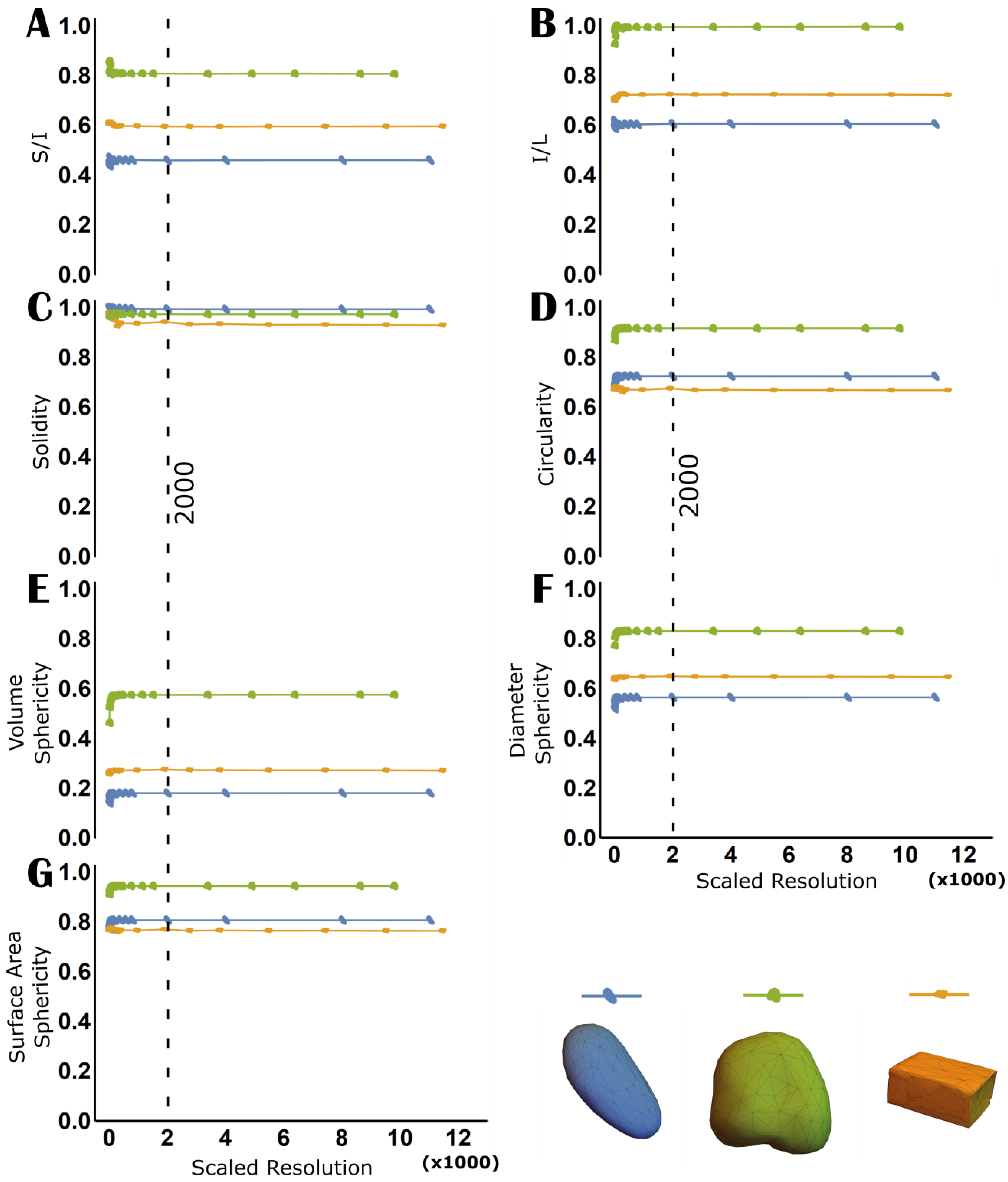
4.3. Three-dimensional Model Resolution

Imaging methods need to have a minimum resolution defined for reproducible particle shape and size analysis. For optical-image-based 2D shape analysis, several studies have identified minimum resolution for shape quantification [42,69,70,71,72]. Similarly, there are studies that have investigated the effect of computed tomography (CT) image voxel resolution on the estimation of rock properties [73,74]. However, there is a lack of research on the effect of image resolution on 3D shape analysis in the case of SfM photogrammetry. This study defines a resolution metric, i.e., scaled resolution for 3D models obtained from SfM photogrammetry. A minimum scaled resolution of 2000 points is estimated for accurately calculating the 3D shape and size parameters implemented in this paper. The minimum model resolution is an important step forward towards standardising SfM photogrammetry for 3D shape and size analysis. Furthermore, it will be vital in applying the photogrammetry and shape analysis methodology for varying sample sizes (see Section 4.5) as well as decreasing the time and high-specification computational requirements to generate overly detailed 3D models.

4.4. Comparison with other Methods

While manual measurement of particle size is quick and easy to perform, measurement of 3D particle shape manually suffers from particular limitations. Physical parameters such as surface area and volume are tedious and sometimes impractical to calculate using manual methods. Therefore, 3D particle shape analysis has been, until recently, limited to the calculation of shape parameters dependent solely on the principal axes’ measurement (see Table 1 (2 to 11)). The user-friendly and cheap 3D photogrammetry presented here can empower users to not only calculate the size and shape parameters used here but also perform complex shape analysis. For example, spherical harmonics analysis [75,76] can be performed on the point cloud data of the 3D models.

The SfM photogrammetry technique described in this paper renders surficial 3D information. On the other hand, X-ray computed tomography (CT) has been used in the past for internal as well as surficial 3D data. The major difference between the two techniques is the type of data obtained using each technique, i.e., optical for SfM photogrammetry versus X-ray attenuation index for computed tomography. Thus, it is possible to obtain information about the internal structure and material properties of a particle using CT imaging. In contrast, obtaining internal material and structure information of a particle is out of the scope of the methodology described here.

While SfM photogrammetry requires a cheap and readily available digital camera to obtain images, the instrumentation cost is much higher for CT scanning (>100 k USD) when compared to the method carried out herein (common mobile phone, ~500 Euro; Agisoft educational licence approx. ~500 Euro). It is worth noting that the SfM photogrammetry workflow can be carried out in a number of open-source software packages such as MicMap (French National Geographic Institute; https://micmac.ensg.eu/ (accessed on 4 May 2023)) and VisualSFM (http://ccwu.me/vsfm (accessed on 4 May 2023)). Image acquisition for SfM photogrammetry can be performed anywhere—in the field as well as in a laboratory setting. On the other hand, due to the instrumentation involved, CT scanning is restricted to the laboratory setting. In summary, CT scanning ought to be used where particle material or internal structure information is required, and SfM photogrammetry provides a cheap and flexible option for particle shape analysis.

4.5. Applications beyond Hand-Held Samples

The SfM photogrammetry approach can be applied to images and analyses sand-sized particles [52]. This study provides a reference for the minimum model resolution to be used to perform particle shape analysis. Future work entails benchmarking SfM photogrammetry methodology for 3D imaging of sand-sized particles using microphotograph images. The scaled resolution proposed and defined in this study will be essential in making sure any such study encompasses the minimum model resolution for particle characterisation.

There are several avenues for the application of 3D shape and size analysis of sedimentary particles such as investigating the depositional environment [77], bedload transport [12], and bulk rock properties [16,17]. Furthermore, once standardised for microscale applications, 3D imaging and morphological analysis can be applied to microfossils. There is an active interest in developing imaging and automatic recognition software for microfossils such as foraminifera [78,79] for research and industrial applications. On the other hand, larger boulders and immovable objects could also be imaged in the field for subsequent processing and analysis in the laboratory [80,81]. This study provides a solid foundation for extending 3D photogrammetry applications to samples of varying sizes and for a variety of research objectives.

In recent years, 3D printing has been used for geological research and teaching [82,83,84]. Using the SfM photogrammetry method, 3D models can be easily created for the 3D printing of geological specimens. Three-dimensional particle shape information can be used for numerical studies involving DEM [85]. Furthermore, surface roughness in granular matter can be studied using the 3D models generated by SfM photogrammetry. Thus, 3D particle imaging and processing using SfM provides a powerful, cheap, and versatile tool that can be applied for numerous applications within geoscientific disciplines.

5. Conclusions

This study presents a low-cost, versatile methodology for 3D imaging of particles using SfM photogrammetry. Using a readily available smartphone device, multiple 2D images were captured and processed to construct 3D image models of a total of 16 samples (13 natural and 3 man-made reference samples). A comprehensive set of 16 commonly used size and shape parameters were computed for the samples. The variation in the results provides an expected range of values for the shape parameters for natural samples which can be used as a reference for future 3D shape analysis studies.

This study develops a concept of minimum scaled resolution, independent of particle size, for 3D shape analysis. Scaled resolution is thus proposed here as the number of unique points in a 3D model point cloud divided by the normalised surface area of the 3D model. For the size and shape parameters used in this study, a minimum scaled resolution was determined as 2000 points. Thus, samples with particle sizes ranging from sand to a boulder can be all compared for various 3D shape parameters when they are imaged above the minimum scaled resolution.

In academia, a range of scientific disciplines (e.g., geosciences, biological sciences, and civil engineering) will benefit from the 3D shape and size methodology proposed here. Additionally, 3D shape and size analysis is of immense interest to our colleagues in industry for commercial applications (e.g., the construction and material industries). Therefore, the methodology presented in this study hopes to open avenues for various applications of 3D particle imaging and characterisation.

References

1. Blott, S.J.; Pye, K. Particle Shape: A Review and New Methods of Characterization and Classification. Sedimentology 2008, 55, 31–63. [Google Scholar] [CrossRef]
2. Chávez, G.M.; Castillo-Rivera, F.; Montenegro-Ríos, J.A.; Borselli, L.; Rodríguez-Sedano, L.A.; Sarocchi, D. Fourier Shape Analysis, FSA: Freeware for Quantitative Study of Particle Morphology. J. Volcanol. Geotherm. Res. 2020, 404, 107008. [Google Scholar] [CrossRef]
3. Dürig, T.; Ross, P.-S.; Dellino, P.; White, J.D.L.; Mele, D.; Comida, P.P. A Review of Statistical Tools for Morphometric Analysis of Juvenile Pyroclasts. Bull. Volcanol. 2021, 83, 79. [Google Scholar] [CrossRef]
4. Güler, C.; Beyhan, B.; Tağa, H. PolyMorph-2D: An Open-Source GIS Plug-in for Morphometric Analysis of Vector-Based 2D Polygon Features. Geomorphology 2021, 386, 107755. [Google Scholar] [CrossRef]
5. Mulchrone, K.F.; McCarthy, D.J.; Meere, P.A. Mathematica Code for Image Analysis, Semi-Automatic Parameter Extraction and Strain Analysis. Comput. Geosci. 2013, 61, 64–70. [Google Scholar] [CrossRef]
6. Higgins, M.D. Quantitative Textural Measurements in Igneous and Metamorphic Petrology; Cambridge University Press: Cambridge, UK, 2006; ISBN 978-0-521-84782-7. [Google Scholar]
7. Campaña, I.; Benito-Calvo, A.; Pérez-González, A.; Bermúdez de Castro, J.M.; Carbonell, E. Assessing Automated Image Analysis of Sand Grain Shape to Identify Sedimentary Facies, Gran Dolina Archaeological Site (Burgos, Spain). Sediment. Geol. 2016, 346, 72–83. [Google Scholar] [CrossRef]
8. Eamer, J.B.R.; Shugar, D.H.; Walker, I.J.; Lian, O.B.; Neudorf, C.M. Distinguishing Depositional Setting For Sandy Deposits In Coastal Landscapes Using Grain Shape. J. Sediment. Res. 2017, 87, 1–11. [Google Scholar] [CrossRef]
9. Pantopoulos, G.; Manica, R.; McArthur, A.D.; Kuchle, J. Particle Shape Trends across Experimental Cohesive and Non-Cohesive Sediment Gravity Flow Deposits: Implications for Particle Fractionation and Discrimination of Depositional Settings. Sedimentology 2022, 69, 1495–1518. [Google Scholar] [CrossRef]
10. Suzuki, K.; Fujiwara, H.; Ohta, T. The Evaluation of Macroscopic and Microscopic Textures of Sand Grains Using Elliptic Fourier and Principal Component Analysis: Implications for the Discrimination of Sedimentary Environments. Sedimentology 2015, 62, 1184–1197. [Google Scholar] [CrossRef]
11. Tunwal, M.; Mulchrone, K.F.; Meere, P.A. Quantitative Characterisation of Grain Shape: Implications for Textural Maturity Analysis and Discrimination between Depositional Environments. Sedimentology 2018, 65, 1761–1776. [Google Scholar] [CrossRef]
12. Deal, E.; Venditti, J.G.; Benavides, S.J.; Bradley, R.; Zhang, Q.; Kamrin, K.; Perron, J.T. Grain Shape Effects in Bed Load Sediment Transport. Nature 2023, 613, 298–302. [Google Scholar] [CrossRef] [PubMed]
13. Novák-Szabó, T.; Sipos, A.Á.; Shaw, S.; Bertoni, D.; Pozzebon, A.; Grottoli, E.; Sarti, G.; Ciavola, P.; Domokos, G.; Jerolmack, D.J. Universal Characteristics of Particle Shape Evolution by Bed-Load Chipping. Sci. Adv. 2018, 4, eaao4946. [Google Scholar] [CrossRef] [PubMed] [Green Version]
14. Szabó, T.; Domokos, G.; Grotzinger, J.P.; Jerolmack, D.J. Reconstructing the Transport History of Pebbles on Mars. Nat. Commun. 2015, 6, 8366. [Google Scholar] [CrossRef] [PubMed] [Green Version]
15. Vaughan, A.; Minitti, M.E.; Cardarelli, E.L.; Johnson, J.R.; Kah, L.C.; Pilleri, P.; Rice, M.S.; Sephton, M.; Horgan, B.H.N.; Wiens, R.C.; et al. Regolith of the Crater Floor Units, Jezero Crater, Mars: Textures, Composition, and Implications for Provenance. J. Geophys. Res. Planets 2023, 128, e2022JE007437. [Google Scholar] [CrossRef]
16. Payton, R.L.; Chiarella, D.; Kingdon, A. The Influence of Grain Shape and Size on the Relationship between Porosity and Permeability in Sandstone: A Digital Approach. Sci. Rep. 2022, 12, 7531. [Google Scholar] [CrossRef]
17. Yan, Y.; Zhang, L.; Luo, X.; Liu, K.; Jia, T.; Lu, Y. Influence of the Grain Shape and Packing Texture on the Primary Porosity of Sandstone: Insights from a Numerical Simulation. Sedimentology 2023. Online Version. [Google Scholar] [CrossRef]
18. Markwitz, V.; Kirkland, C.L. Source to Sink Zircon Grain Shape: Constraints on Selective Preservation and Significance for Western Australian Proterozoic Basin Provenance. Geosci. Front. 2018, 9, 415–430. [Google Scholar] [CrossRef]
19. Barrett, P.J. The Shape of Rock Particles, a Critical Review. Sedimentology 1980, 27, 291–303. [Google Scholar] [CrossRef]
20. Jia, X.; Garboczi, E.J. Advances in Shape Measurement in the Digital World. Particuology 2016, 26, 19–31. [Google Scholar] [CrossRef] [Green Version]
21. Wadell, H. Volume, Shape, and Roundness of Rock Particles. J. Geol. 1932, 40, 443–451. [Google Scholar] [CrossRef]
22. Wentworth, C.K. A Laboratory and Field Study of Cobble Abrasion. J. Geol. 1919, 27, 507–521. [Google Scholar] [CrossRef] [Green Version]
23. Krumbein, W.C. Measurement and Geological Significance of Shape and Roundness of Sedimentary Particles. J. Sediment. Petrol. 1941, 11, 64–72. [Google Scholar] [CrossRef]
24. Powers, M.C. A New Roundness Scale for Sedimentary Particles. J. Sediment. Petrol. 1953, 23, 117–119. [Google Scholar] [CrossRef]
25. Blatt, H. Sedimentary Petrology, 2nd ed.; W. H. Freeman and Company: New York, NY, USA, 1992. [Google Scholar]
26. Blatt, H.; Middleton, G.V.; Murray, R.C. Origin of Sedimentary Rocks; Prentice-Hall Inc.: Hoboken, NJ, USA, 1972. [Google Scholar]
27. Heilbronner, R.; Barrett, S. Image Analysis in Earth Sciences: Microstructures and Textures of Earth Materials; Springer: Berlin/Heidelberg, Germany, 2014; ISBN 3-642-10343-X. [Google Scholar]
28. Roduit, N. JMicroVision: A Multipurpose Image Analysis Software Tool. Ph.D. Thesis, University of Geneva, Geneva, Switzerland, 2007. [Google Scholar]
29. Roussillon, T.; Piégay, H.; Sivignon, I.; Tougne, L.; Lavigne, F. Automatic Computation of Pebble Roundness Using Digital Imagery and Discrete Geometry. Comput. Geosci. 2009, 35, 1992–2000. [Google Scholar] [CrossRef]
30. Schneider, C.A.; Rasband, W.S.; Eliceiri, K.W. NIH Image to ImageJ: 25 Years of Image Analysis. Nat. Methods 2012, 9, 671–675. [Google Scholar] [CrossRef]
31. Tunwal, M.; Mulchrone, K.F.; Meere, P.A. Image Based Particle Shape Analysis Toolbox (IPSAT). Comput. Geosci. 2020, 135, 104391. [Google Scholar] [CrossRef]
32. Alshibli, K.A.; Druckrey, A.M.; Al-Raoush, R.I.; Weiskittel, T.; Lavrik, N.V. Quantifying Morphology of Sands Using 3D Imaging. J. Mater. Civ. Eng. 2015, 27, 04014275. [Google Scholar] [CrossRef]
33. Komba, J.J.; Anochie-Boateng, J.K.; van der Merwe Steyn, W. Analytical and Laser Scanning Techniques to Determine Shape Properties of Aggregates. Transp. Res. Rec. 2013, 2335, 60–71. [Google Scholar] [CrossRef] [Green Version]
34. Li, R.; Lu, W.; Chen, M.; Wang, G.; Xia, W.; Yan, P. Quantitative Analysis of Shapes and Specific Surface Area of Blasted Fragments Using Image Analysis and Three-Dimensional Laser Scanning. Int. J. Rock Mech. Min. Sci. 2021, 141, 104710. [Google Scholar] [CrossRef]
35. Zheng, J.; Sun, Q.; Zheng, H.; Wei, D.; Li, Z.; Gao, L. Three-Dimensional Particle Shape Characterizations from Half Particle Geometries. Powder Technol. 2020, 367, 122–132. [Google Scholar] [CrossRef]
36. Chmielowska, D.; Woronko, B.; Dorocki, S. Applicability of Automatic Image Analysis in Quartz-Grain Shape Discrimination for Sedimentary Setting Reconstruction. Catena 2021, 207, 105602. [Google Scholar] [CrossRef]
37. Martewicz, J.; Kalińska, E.; Weckwerth, P. What Hides in the Beach Sand? A Multiproxy Approach and New Textural Code to Recognition of Beach Evolution on the Southern and Eastern Baltic Sea Coast. Sediment. Geol. 2022, 435, 106154. [Google Scholar] [CrossRef]
38. van Buuren, U.; Prins, M.A.; Wang, X.; Stange, M.; Yang, X.; van Balen, R.T. Fluvial or Aeolian? Unravelling the Origin of the Silty Clayey Sediment Cover of Terraces in the Hanzhong Basin (Qinling Mountains, Central China). Geomorphology 2020, 367, 107294. [Google Scholar] [CrossRef]
39. Varga, G.; Kovács, J.; Szalai, Z.; Cserháti, C.; Újvári, G. Granulometric Characterization of Paleosols in Loess Series by Automated Static Image Analysis. Sediment. Geol. 2018, 370, 1–14. [Google Scholar] [CrossRef]
40. Sochan, A.; Zieliński, P.; Bieganowski, A. Selection of Shape Parameters That Differentiate Sand Grains, Based on the Automatic Analysis of Two-Dimensional Images. Sediment. Geol. 2015, 327, 14–20. [Google Scholar] [CrossRef]
41. Szmańda, J.B.; Witkowski, K. Morphometric Parameters of Krumbein Grain Shape Charts—A Critical Approach in Light of the Automatic Grain Shape Image Analysis. Minerals 2021, 11, 937. [Google Scholar] [CrossRef]
42. Tunwal, M.; Mulchrone, K.F.; Meere, P.A. A New Approach to Particle Shape Quantification Using the Curvature Plot. Powder Technol. 2020, 374, 377–388. [Google Scholar] [CrossRef]
43. Snavely, N.; Simon, I.; Goesele, M.; Szeliski, R.; Seitz, S.M. Scene Reconstruction and Visualization From Community Photo Collections. Proc. IEEE 2010, 98, 1370–1390. [Google Scholar] [CrossRef] [Green Version]
44. Lowe, D.G. Distinctive Image Features from Scale-Invariant Keypoints. Int. J. Comput. Vis. 2004, 60, 91–110. [Google Scholar] [CrossRef]
45. Carrivick, J.L.; Smith, M.W.; Quincey, D.J. Structure from Motion in the Geosciences; John Wiley & Sons: Hoboken, NJ, USA, 2016; ISBN 1-118-89583-5. [Google Scholar]
46. Lim, A.; Wheeler, A.J.; Price, D.M.; O’Reilly, L.; Harris, K.; Conti, L. Influence of Benthic Currents on Cold-Water Coral Habitats: A Combined Benthic Monitoring and 3D Photogrammetric Investigation. Sci. Rep. 2020, 10, 19433. [Google Scholar] [CrossRef]
47. Pizarro, O.; Friedman, A.; Bryson, M.; Williams, S.B.; Madin, J. A Simple, Fast, and Repeatable Survey Method for Underwater Visual 3D Benthic Mapping and Monitoring. Ecol. Evol. 2017, 7, 1770–1782. [Google Scholar] [CrossRef] [PubMed]
48. Westoby, M.J.; Brasington, J.; Glasser, N.F.; Hambrey, M.J.; Reynolds, J.M. ‘Structure-from-Motion’ Photogrammetry: A Low-Cost, Effective Tool for Geoscience Applications. Geomorphology 2012, 179, 300–314. [Google Scholar] [CrossRef] [Green Version]
49. Hixon, S.W.; Lipo, C.P.; Hunt, T.L.; Lee, C. Using Structure from Motion Mapping to Record and Analyze Details of the Colossal Hats (Pukao) of Monumental Statues on Rapa Nui (Easter Island). Adv. Archaeol. Pract. 2018, 6, 42–57. [Google Scholar] [CrossRef] [Green Version]
50. Cirillo, D.; Cerritelli, F.; Agostini, S.; Bello, S.; Lavecchia, G.; Brozzetti, F. Integrating Post-Processing Kinematic (PPK)–Structure-from-Motion (SfM) with Unmanned Aerial Vehicle (UAV) Photogrammetry and Digital Field Mapping for Structural Geological Analysis. ISPRS Int. J. Geo-Inf. 2022, 11, 437. [Google Scholar] [CrossRef]
51. Bello, S.; Scott, C.P.; Ferrarini, F.; Brozzetti, F.; Scott, T.; Cirillo, D.; de Nardis, R.; Arrowsmith, J.R.; Lavecchia, G. High-Resolution Surface Faulting from the 1983 Idaho Lost River Fault Mw 6.9 Earthquake and Previous Events. Sci. Data 2021, 8, 68. [Google Scholar] [CrossRef]
52. Xie, W.-Q.; Zhang, X.-P.; Yang, X.-M.; Liu, Q.-S.; Tang, S.-H.; Tu, X.-B. 3D Size and Shape Characterization of Natural Sand Particles Using 2D Image Analysis. Eng. Geol. 2020, 279, 105915. [Google Scholar] [CrossRef]
53. Harris, A.L.; Haselock, P.J.; Kennedy, M.J.; Mendum, J.R.; Long, C.B.; Winchester, J.A.; Tanner, P.W.G. The Dalradian Supergroup in Scotland, Shetland and Ireland. In A Revised Correlation of Pre-Cambrian Rocks in the British Isles; Gibbons, W., Harris, A.L., Eds.; Geological Society of London: London, UK, 1994; Volume 22, ISBN 978-1-897799-11-6. [Google Scholar]
54. de Oliveira, L.M.C.; Lim, A.; Conti, L.A.; Wheeler, A.J. 3D Classification of Cold-Water Coral Reefs: A Comparison of Classification Techniques for 3D Reconstructions of Cold-Water Coral Reefs and Seabed. Front. Mar. Sci. 2021, 8, 640713. [Google Scholar] [CrossRef]
55. Price, D.M.; Robert, K.; Callaway, A.; Lo lacono, C.; Hall, R.A.; Huvenne, V.A.I. Using 3D Photogrammetry from ROV Video to Quantify Cold-Water Coral Reef Structural Complexity and Investigate Its Influence on Biodiversity and Community Assemblage. Coral Reefs 2019, 38, 1007–1021. [Google Scholar] [CrossRef] [Green Version]
56. Wentworth, C.K. The Shapes of Beach Pebbles; US Government Printing Office: Washington, DC, USA, 1922.
57. Pye, W.D.; Pye, M.H. Sphericity Determinations of Pebbles and Sand Grains. J. Sediment. Res. 1943, 13, 28–34. [Google Scholar] [CrossRef]
58. Corey, A.T. Influence of Shape on the Fall Velocity of Sand Grains; Colorado A & M College: Fort Collins, CO, USA, 1949. [Google Scholar]
59. Folk, R.L. Student Operator Error in Determination of Roundness, Sphericity, and Grain Size. J. Sediment. Res. 1955, 25, 297–301. [Google Scholar] [CrossRef]
60. Sneed, E.D.; Folk, R.L. Pebbles in the Lower Colorado River, Texas a Study in Particle Morphogenesis. J. Geol. 1958, 66, 114–150. [Google Scholar] [CrossRef]
61. Aschenbrenner, B.C. A New Method of Expressing Particle Sphericity. J. Sediment. Res. 1956, 26, 15–31. [Google Scholar]
62. Janke, N.C. Effect of Shape upon the Settling Vellocity of Regular Convex Geometric Particles. J. Sediment. Res. 1966, 36, 370–376. [Google Scholar] [CrossRef]
63. Dobkins, J.E.; Folk, R.L. Shape Development on Tahiti-Nui. J. Sediment. Res. 1970, 40, 1167–1203. [Google Scholar]
64. Mora, C.F.; Kwan, A.K.H. Sphericity, Shape Factor, and Convexity Measurement of Coarse Aggregate for Concrete Using Digital Image Processing. Cem. Concr. Res. 2000, 30, 351–358. [Google Scholar] [CrossRef]
65. Riley, N.A. Projection Sphericity. J. Sediment. Res. 1941, 11, 94–97. [Google Scholar]
66. Wadell, H. Sphericity and Roundness of Rock Particles. J. Geol. 1933, 41, 310–331. [Google Scholar] [CrossRef]
67. Kuo, C.-Y.; Freeman, R.B. Imaging Indices for Quantification of Shape, Angularity, and Surface Texture of Aggregates. Transp. Res. Rec. 2000, 1721, 57–65. [Google Scholar] [CrossRef]
68. Zhang, C.; Chen, T. Efficient Feature Extraction for 2D/3D Objects in Mesh Representation. In Proceedings of the 2001 International Conference on Image Processing (Cat. No.01CH37205), Thessaloniki, Greece, 7–10 October 2001; Volume 3, pp. 935–938. [Google Scholar]
69. Kröner, S.; Doménech Carbó, M.T. Determination of Minimum Pixel Resolution for Shape Analysis: Proposal of a New Data Validation Method for Computerized Images. Powder Technol. 2013, 245, 297–313. [Google Scholar] [CrossRef]
70. Sun, Q.; Zheng, J.; Coop, M.R.; Altuhafi, F.N. Minimum Image Quality for Reliable Optical Characterizations of Soil Particle Shapes. Comput. Geotech. 2019, 114, 103110. [Google Scholar] [CrossRef]
71. Zingg, T. Beitrag zur Schotteranalyse. Ph.D. Thesis, ETH Zurich, Zürich, Switzerland, 1935. [Google Scholar]
72. Đuriš, M.; Arsenijević, Z.; Jaćimovski, D.; Kaluđerović Radoičić, T. Optimal Pixel Resolution for Sand Particles Size and Shape Analysis. Powder Technol. 2016, 302, 177–186. [Google Scholar] [CrossRef]
73. Bazaikin, Y.; Gurevich, B.; Iglauer, S.; Khachkova, T.; Kolyukhin, D.; Lebedev, M.; Lisitsa, V.; Reshetova, G. Effect of CT Image Size and Resolution on the Accuracy of Rock Property Estimates. J. Geophys. Res. Solid Earth 2017, 122, 3635–3647. [Google Scholar] [CrossRef]
74. Guan, K.M.; Nazarova, M.; Guo, B.; Tchelepi, H.; Kovscek, A.R.; Creux, P. Effects of Image Resolution on Sandstone Porosity and Permeability as Obtained from X-ray Microscopy. Transp. Porous Med. 2019, 127, 233–245. [Google Scholar] [CrossRef]
75. Bullard, J.W.; Garboczi, E.J. Defining Shape Measures for 3D Star-Shaped Particles: Sphericity, Roundness, and Dimensions. Powder Technol. 2013, 249, 241–252. [Google Scholar] [CrossRef]
76. Taylor, M.A.; Garboczi, E.J.; Erdogan, S.T.; Fowler, D.W. Some Properties of Irregular 3-D Particles. Powder Technol. 2006, 162, 1–15. [Google Scholar] [CrossRef]
77. Dadd, K.; Foley, K. A Shape and Compositional Analysis of Ice-Rafted Debris in Cores from IODP Expedition 323 in the Bering Sea. Deep. Sea Res. Part II Top. Stud. Oceanogr. 2016, 125, 191–201. [Google Scholar] [CrossRef]
78. Carvalho, L.E.; Fauth, G.; Baecker Fauth, S.; Krahl, G.; Moreira, A.C.; Fernandes, C.P.; von Wangenheim, A. Automated Microfossil Identification and Segmentation Using a Deep Learning Approach. Mar. Micropaleontol. 2020, 158, 101890. [Google Scholar] [CrossRef]
79. Mitra, R.; Marchitto, T.M.; Ge, Q.; Zhong, B.; Kanakiya, B.; Cook, M.S.; Fehrenbacher, J.S.; Ortiz, J.D.; Tripati, A.; Lobaton, E. Automated Species-Level Identification of Planktic Foraminifera Using Convolutional Neural Networks, with Comparison to Human Performance. Mar. Micropaleontol. 2019, 147, 16–24. [Google Scholar] [CrossRef]
80. Ehlmann, B.L.; Viles, H.A.; Bourke, M.C. Quantitative Morphologic Analysis of Boulder Shape and Surface Texture to Infer Environmental History: A Case Study of Rock Breakdown at the Ephrata Fan, Channeled Scabland, Washington. J. Geophys. Res. Earth Surf. 2008, 113, F02012. [Google Scholar] [CrossRef] [Green Version]
81. Chen, Z.; Scott, C.; Keating, D.; Clarke, A.; Das, J.; Arrowsmith, R. Quantifying and Analysing Rock Trait Distributions of Rocky Fault Scarps Using Deep Learning. Earth Surf. Process. Landf. 2023, 48, 1234–1250. [Google Scholar] [CrossRef]
82. Horowitz, S.S.; Schultz, P.H. Printing Space: Using 3D Printing of Digital Terrain Models in Geosciences Education and Research. J. Geosci. Educ. 2014, 62, 138–145. [Google Scholar] [CrossRef]
83. Wei, D.; Wang, Z.; Pereira, J.-M.; Gan, Y. Permeability of Uniformly Graded 3D Printed Granular Media. Geophys. Res. Lett. 2021, 48, e2020GL090728. [Google Scholar] [CrossRef]
84. Xia, Y.; Zhang, C.; Zhou, H.; Hou, J.; Su, G.; Gao, Y.; Liu, N.; Singh, H.K. Mechanical Behavior of Structurally Reconstructed Irregular Columnar Jointed Rock Mass Using 3D Printing. Eng. Geol. 2020, 268, 105509. [Google Scholar] [CrossRef]
85. Zhang, T.; Zhang, C.; Zou, J.; Wang, B.; Song, F.; Yang, W. DEM Exploration of the Effect of Particle Shape on Particle Breakage in Granular Assemblies. Comput. Geotech. 2020, 122, 103542. [Google Scholar] [CrossRef]
Figure 1. Sample images S1–S16 for the 16 samples used in the study. S1–S13 are natural samples. S14, S15, and S16 are a matchbox, a chopping box, and a pen representing a cuboid, a platy, and a rod shape, respectively. The white line refers to a 1 cm scale.
Geosciences 13 00190 g001
Figure 2. Schematic of camera position relative to the object of interest to achieve sufficient (>60%) overlap for the structure from motion processing utilised for this study.
Geosciences 13 00190 g002
Figure 3. Figure showing different steps for shape and size calculation. (A) Sample S10 (from Figure 1); (B) resultant 3D model; (C) 3D point cloud; (D) minimum oriented cuboid over the sample; (E) smallest bounding sphere over the sample; and (F) 3D convex hull of the sample.
Geosciences 13 00190 g003
Figure 4. Three-dimensional models for samples S1–S16. The 3D models along with their position and orientation correspond to the sample images from Figure 1.
Geosciences 13 00190 g004
Figure 5. Three-dimensional models of samples 1–8 in the inlet on right and samples 9–16 on the left. Sample values on the Zingg’s scatter for S/I versus I/L plot along with contour of: (A) Wentworth flatness index; (B) Krumbein intercept sphericity; (C) Corey shape factor; (D) maximum projection sphericity; (E) Aschenbrenner working sphericity; (F) Aschenbrenner shape factor; (G) Janke form factor; (H) Oblate–Prolate Index.
Geosciences 13 00190 g005
Figure 6. Three-dimensional models of samples 1–8 in the inlet on the right and samples 9–16 on the left. Sample values for solidity, circularity, volume sphericity, diameter sphericity, and surface area sphericity.
Geosciences 13 00190 g006
Figure 7. Values for samples S8, S10, and S14 measured at varying scaled resolutions for the shape parameters: (A) S/I; (B) I/L; (C) solidity; (D) circularity; (E) volume sphericity; (F) diameter sphericity; and (G) surface area sphericity.
Geosciences 13 00190 g007