

Spatiotemporal Evolution of Ground Subsidence and Extensional Basin Bedrock Organization: An Application of Multitemporal Multi-Satellite SAR Interferometry


Abstract
1. Introduction


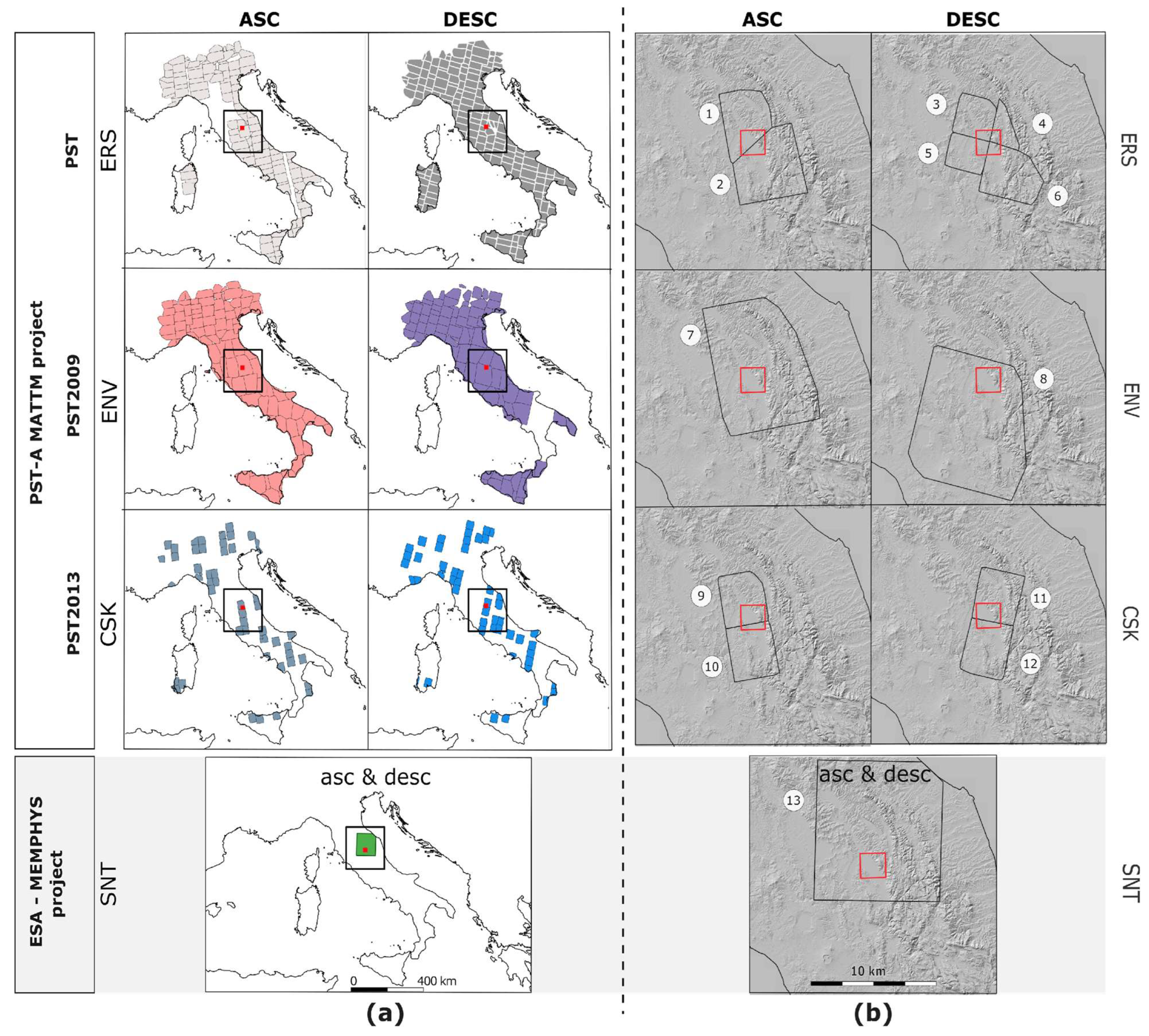
| ERS | ENV | CSK | SNT | |||||
|---|---|---|---|---|---|---|---|---|
| ASC | DESC | ASC | DESC | ASC | DESC | ASC | DESC | |
| Numb of PS | 4.378.310 | 9.438.651 | 15.359.988 | 12.895.230 | 65.019.955 | 63.735.666 | 611.986 | 721.982 |
| Numb. of Clusters | 117 | 201 | 110 | 95 | 56 | 56 | 1 | 1 |
| PS/kmq (avg.) | 2.150,1 | 5.905,2 | 5.344,1 | 4.495,3 | 47.774,7 | 46.447,8 | 51.58 | 60.85 |
| Max | 218.468 | 264.282 | 747.622 | 756.312 | 4.601.190 | 4.242.770 | ||
| Min | 881 | 518 | 205 | 258 | 20.969 | 4.940 | ||
| Mean | 37.744 | 47.193 | 139.635 | 135.739 | 1.154.140 | 1.051.230 | ||
| Median | 27.902 | 34.248 | 72.690 | 70.995 | 872.943 | 893.517 | ||
| ERS 1-2 | ENV | CSK | SNT1 | |
|---|---|---|---|---|
| Band (wavelen. cm) | C-band (5.6) | C-band (5.6) | X-Band (3.1) | C-band (5.6) |
| Operation mode | SAR/IM | SAR/IM | HIMAGE (Stripmap) | TOPSAR |
| Revisit cycle days | 35 | 35 | 16 | 12 |
| Look angle | 23° | 23° | 25–57° | 30.5° |
| Swath km | 100 | 100 | 40 | 250 |
| ASC n. images | 35 | 51 | 40 | 48 |
| ASC first image | 2 April 1995 | 2 December 2002 | 9 May 2011 | 25 October 2014 |
| ASC last image | 23 October 2000 | 24 May 2010 | 30 March 2014 | 21 August 2016 |
| DESC n. images | 56 | 37 | 30 | 42 |
| DESC first image | 21 April 1992 | 10 October 2003 | 29 July 2011 | 24 October 2014 |
| DESC last image | 29 December 2000 | 25 June 2010 | 16 April 2014 | 1 September 2016 |
| Orbit | Project ID | Cluster ID | Number in Figure 1b | |
|---|---|---|---|---|
| ERS 1-2 | ASC | PST | ERS_T401_F858_CL003_SPELLO ERS_T401_F858_CL004_SPOLETO | 1 2 |
| DESC | PST | ERS_T351_F2745_CL002_PERUGIA ERS_T79_F2748_CL001_GUALDO ERS_T79_F2748_CL003_SPOLETO ERS_T351_F2745_CL001_MARSCIANO | 3 4 5 6 | |
| ENV | ASC | PST2009 | ENVISAT_T401_F858_CL001_ASSISI | 7 |
| DESC | PST2009 | ENVISAT_T351_F2745_CL001_TERNI | 8 | |
| CSK | ASC | PST2013 | CSK_F_44_PERUGIA_A_CL001 CSK_F_43_SPOLETO_A_CL001 | 9 10 |
| DESC | PST2013 | CSK_F_46_SPOLETO_D_CL001 CSK_F_45_GUALDOTADINO_D_CL001 | 11 12 | |
| SNT | ASC | SqueeSAR | S1_T117_A_33 | 13 |
| DESC | SqueeSAR | S1_T95_D_32 | 13 |
2. Case Study
3. Materials and Methods
4. Discussion
5. Conclusions
Author Contributions
Funding
Data Availability Statement
Acknowledgments
Conflicts of Interest
References
- Casu, F.; Manunta, M.; Agramb, P.S.; Crippen, R.E. Big Remotely Sensed Data: Tools, applications and experiences. Remote Sens. Environ. 2017, 202, 1–2. [Google Scholar] [CrossRef]
- De Luca, C.; Zinno, I.; Manunta, M.; Lanari, R.; Casu, F. Large areas surface deformation analysis through a cloud computing P-SBAS approach for massive processing of DInSAR time series. Remote Sens. Environ. 2017, 202, 3–17. [Google Scholar] [CrossRef]
- Cigna, F.; Tapete, D. Sentinel-1 Big Data Processing with P-SBAS InSAR in the Geohazards Exploitation Platform: An Experiment on Coastal Land Subsidence and Landslides in Italy. Remote Sens. 2021, 13, 885. [Google Scholar] [CrossRef]
- Costantini, M.; Ferretti, A.; Minati, F.; Falco, S.; Trillo, F.; Colombo, D.; Novali, F.; Malvarosa, F.; Mammone, C.; Vecchioli, F.; et al. Analysis of surface deformations over the whole Italian territory by interferometric processing of ERS, ENVISAT and COSMO-SkyMed radar data. Remote Sens. Environ. 2017, 202, 250–275. [Google Scholar] [CrossRef]
- Solari, L.; Del Soldato, M.; Bianchini, S.; Ciampalini, A.; Ezquerro, P.; Montalti, R.; Raspini, F.; Moretti, S. From ERS 1/2 to Sentinel-1: Subsidence Monitoring in Italy in the Last Two Decades. Front. Earth Sci. 2018, 6, 149. [Google Scholar] [CrossRef]
- Terzaghi, K.V. Relation between soil mechanics and foundation engineering. In Proceedings of the 1936 International Conference on Soil Mechanics and Foundation Engineering, Boston, MA, USA, 22–26 June 1936. [Google Scholar]
- Cigna, F.; Jordan, H.; Bateson, L.; McCormack, H.; Roberts, C. Natural and Anthropogenic Geohazards in Greater London Observed from Geological and ERS-1/2 and ENVISAT Persistent Scatterers Ground Motion Data: Results from the EC FP7-SPACE PanGeo Project. Pure Appl. Geophys. 2015, 172, 2965–2995. [Google Scholar] [CrossRef]
- Dong, S.; Samsonov, S.; Yin, H.; Ye, S.; Cao, Y. Time-series analysis of subsidence associated with rapid urbanisation in Shanghai, China measured with SBAS InSAR method. Environ. Earth Sci. 2014, 72, 677–691. [Google Scholar] [CrossRef]
- Chaussard, E.; Wdowinski, S.; Cabral-Cano, E.; Amelung, F.C. Land subsidence in central Mexico detected by ALOS InSAR time series. Remote Sens. Environ. 2014, 140, 94–106. [Google Scholar] [CrossRef]
- Murgia, F.; Bignami, C.; Brunori, C.A.; Tolomei, C.; Pizzimenti, L. Ground deformations controlled by hidden faults: Multifrequency and multitemporal InSAR techniques for urban hazard monitoring. Remote Sens. 2019, 11, 2246. [Google Scholar] [CrossRef]
- Cigna, F.; Tapete, D. Land subsidence and aquifer-system storage loss in Central Mexico: A quasi-continental investigation with Sentinel-1 InSAR. Geophys. Res. Lett. 2022, 4, e2022GL098923. [Google Scholar] [CrossRef]
- Delgado Blasco, J.M.; Foumelis, M.; Stewart, C.; Hooper, A. Measuring Urban Subsidence in the Rome Metropolitan Area (Italy) with Sentinel-1 SNAP-StaMPS Persistent Scatterer Interferometry. Remote Sens. 2019, 11, 129. [Google Scholar] [CrossRef]
- Stramondo, S.; Saroli, M.; Tolomei, C.; Moro, M.; Doumaz, F.; Pesci, A.; Boschi, E. Surface movements in Bologna (Po Plain-Italy) detected by multitemporal DInSAR. Remote Sens. Environ. 2007, 110, 304–316. [Google Scholar] [CrossRef]
- Antonellini, M.; Giambastiani, B.M.S.; Greggio, N.; Bonzi, L.; Calabrese, L.; Luciani, P.; Perini, L.; Severi, P. Processes governing natural land subsidence in the shallow coastal aquifer of the Ravenna coast, Italy. Catena 2019, 172, 76–86. [Google Scholar] [CrossRef]
- Polcari, M.; Albano, M.; Montuori, A.; Bignami, C.; Tolomei, C.; Pezzo, G.; Falcone, S.; La Piana, C.; Doumaz, F.; Salvi, S.; et al. InSAR Monitoring of Italian Coastline Revealing Natural and Anthropogenic Ground Deformation Phenomena and Future Perspectives. Sustainability 2018, 10, 3152. [Google Scholar] [CrossRef]
- Fiaschi, S.; Fabris, M.; Floris, M.; Achilli, V. Estimation of land subsidence in deltaic areas through differential SAR interferometry: The Po River Delta case study (Northeast Italy). Int. J. Remote Sens. 2018, 39, 8724–8745. [Google Scholar] [CrossRef]
- Teatini, P.; Tosi, L.; Strozzi, T.; Carbognin, L.; Cecconi, G.; Rosselli, R.; Libardo, S. Resolving land subsidence within the Venice Lagoon by persistent scatterer SAR interferometry. J. Phys. Chem. Earth. 2010, 40, 72–79. [Google Scholar] [CrossRef]
- Solari, L.; Ciampalini, A.; Raspini, F.; Bianchini, S.; Moretti, S. PSInSAR Analysis in the pisa urban area (Italy): A case study of subsidence related to stratigraphical factors and urbanization. Remote Sens. 2016, 8, 120. [Google Scholar] [CrossRef]
- Raspini, F.; Cigna, F.; Moretti, S. Multi-temporal mapping of land subsidence at basin scale exploiting Persistent Scatterer Interferometry: Case study of Gioia Tauro plain (Italy). J. Maps 2012, 8, 514–524. [Google Scholar] [CrossRef]
- Cianflone, G.; Tolomei, C.; Brunori, C.A.; Dominici, R. InSAR time series analysis of natural and anthropogenic coastal plain subsidence: The case of Sibari (Southern Italy). Remote Sens. 2016, 7, 16004–16023. [Google Scholar] [CrossRef]
- Brunori, C.A.; Bignami, C.; Albano, M.; Zucca, F.; Samsonov, S.; Groppelli, G.; Norini, G.; Saroli, M.; Stramondo, S. Land subsidence, Ground Fissures and Buried Faults: InSAR Monitoring of Ciudad Guzmán (Jalisco, Mexico). Remote Sens. 2015, 7, 8610–8630. [Google Scholar] [CrossRef]
- Navarro-Hernández, M.I.; Tomás, R.; Lopez-Sanchez, J.M.; Cárdenas-Tristán, A.; Mallorquí, J.J. Spatial analysis of land subsidence in the San Luis Potosí valley induced by aquifer overexploitation using the coherent pixels technique (CPT) and sentinel-1 InSAR observation. Remote Sens. 2020, 12, 3822. [Google Scholar] [CrossRef]
- Gourmelen, N.; Amelung, F.; Casu, F.; Manzo, M.; Lanari, R. Mining-related ground deformation in Crescent Valley, Nevada: Implications for sparse GPS networks. Geophys. Res. Lett. 2007, 34, L09309. [Google Scholar] [CrossRef]
- Cianflone, G.; Tolomei, C.; Brunori, C.A.; Monna, S.; Dominici, R. Landslides and Subsidence Assessment in the Crati Valley (Southern Italy) Using InSAR Data. Geosciences 2018, 8, 67. [Google Scholar] [CrossRef]
- Guzzetti, F.; Manunta, M.; Ardizzone, F.; Pepe, A.; Cardinali, M.; Zeni, G.; Reickenbach, P.; Lanari, R. Analysis of ground deformation detected using the SBAS-DInSAR technique in Umbria, Central Italy. Pure Appl. Geophys. 2009, 166, 1425–1459. [Google Scholar] [CrossRef]
- Scarsella, F. Un raggruppamento di pieghe dell’Appennino umbro-marchigiano. La catena M. Nerone-M. Catria-M. Cucco-M. Penna-Colfiorito-M. Serano. Boll. Serv. Geol. D’italia 1951, 73, 309–320. [Google Scholar]
- Lavecchia, G.; Barchi, M.; Brozzetti, F.; Menichetti, M. Sismicità e tettonica nell’area umbro-marchigiana. Boll. Soc. Geol. It. 1994, 113, 483–500. [Google Scholar]
- Barchi, M.R.; Lemmi, M. NOTE ILLUSTRATIVE della CARTA GEOLOGICA D’ITALIA alla Scala 1:50.000, Foglio 324 Foligno. ISPRA-Servizio Geologico d’Italia. 2015. Available online: https://www.isprambiente.gov.it/Media/carg/note_illustrative/324_Foligno.pdf (accessed on 30 March 2023).
- Tarquini, S.; Isola, I.; Favalli, M.; Battistini, A.; Dotta, G. TINITALY, a Digital Elevation Model of Italy with a 10 meters Cell Size (Version 1.1); Istituto Nazionale di Geofisica e Vulcanologia (INGV): Rome, Italy, 2023. [Google Scholar] [CrossRef]
- Coltorti, M.; Pieruccini, P. Middle-Upper Pliocene ‘compression’ and Middle Pleistocene ‘extension’ in the modelling of the East Tiber Basin (Central Italy): From ‘perched’ to ‘extensional’ basin in the Northern Apennines. Il Quat. 1997, 10, 521–528. [Google Scholar]
- Camerieri, P.; Manconi, D. “Le centuriazioni della Valle Umbra da Spoleto a Perugia”. In Proceedings of the XVII International Congress of Classical Archaeology, Roma, Italy, 22–26 September 2008. [Google Scholar]
- Conti, M.A.; Girotti, O. Il Villafranchiano nel «lago tiberino », ramo sud-occidentale: Schema stratigrafico e tettonico. Geol. Romana 1977, 16, 67–80. [Google Scholar]
- Ambrosetti, P.; Carboni, M.G.; Conti, M.A.; Esu, D.; Girotti, O.; La Monica, G.B.; Landini, B.; Parisi, G. Il Pliocene ed il Pleistocene inferiore del bacino del Fiume Tevere nell’Umbria meridionale. Geogr. Fis. Dinam. Quat. 1987, 10, 10–33. [Google Scholar]
- Basilici, G. Sedimentary facies in an extensional and deep-lacustrine depositional system: The Pliocene Tiberino Basin, Central Italy. Sediment. Geol. 1997, 109, 73–94. [Google Scholar] [CrossRef]
- Bucci, F.; Mirabella, F.; Santangelo, M.; Cardinali, M.; Guzzetti, F. Photogeology of the Montefalco Quaternary basin, Umbria, Central Italy. J. Maps 2016, 12, 314–322. [Google Scholar] [CrossRef]
- Mi, G. NA. (1962)—“Ligniti e torbe dell‘Italia continentale”; Geomineraria Nazionale: Roma, Italy, 1963; p. 319. (In Italian) [Google Scholar]
- Cardinali, M.; Antonini, G.; Reichenbach, P.; Guzzetti, F. Photo-geological and landslide inventory map for the Upper Tevere River basin. CNR, Gruppo Nazionale per la Difesa dalle Catastrofi Idrogeologiche, Publication n. 2154, scale 1:100,000. 2001. Available online: http://geomorphology.irpi.cnr.it/publications/repository/public/maps/UTR-data.jpg/view (accessed on 30 March 2023).
- Martinetto, E.; Bertini, A.; Basilici, G.; Baldanza, A.; Bizzarri, R.; Cherin, M.; Gentili, S.; Pontini, M.R. The plant record of the Dunarobba and Pietrafitta sites in the plio-pleistocene palaeoenvironmental context of central Italy. Alp. Mediterr. Quat. 2014, 27, 29–72. [Google Scholar]
- Mutti, E.; Ricci Lucchi, F. Turbidites of the northern Apennines: Introduction to facies analysis. Int. Geol. Rev. 1978, 20, 125–166. [Google Scholar] [CrossRef]
- Centamore, E.; Deiana, G.; Micarelli, A.; Potetti, M. Il Trias-Paleogene delle Marche. Studi. Geologici. Camerti. 1986, Volume Speciale, 9–27. [Google Scholar]
- Cresta, S.; Monechi, S.; Parisi, G.; Baldanza, A.; Reale, V. Stratigrafia del Mesozoico e Cenozoico nell’area umbro-marchigiana. Itinerari geologici sull’Appennino Umbro-marchigiano. In Mem. Descr. Della Carta Geol. D’it.; 1989; 39. Available online: https://www.isprambiente.gov.it/it/pubblicazioni/periodici-tecnici/memorie-descrittive-della-carta-geologica-ditalia/stratigrafia-del-mesozoico-e-cenozoico-nellarea-umbro-marchigiana (accessed on 30 March 2023)(Available only in electronic format, In Italian).
- Barchi, M. The Neogene-quaternary evolution of the Northern ApeREFines: Crustal structure, style of deformation and seismicity. In The Geology of Italy, Journal of the Virtual Explorer, Electronic Edition; Beltrando, M., Peccerillo, A., Matte, M., Conticelli, S., Doglioni, C., Eds.; Virtual Explorer Pty Ltd: Clear Range, Australia, 2010; Volume 36, p. 10. [Google Scholar]
- Pucci, S.; Mirabella, F.; Pazzaglia, F.; Barchi, M.R.; Melelli, L.; Tuccimei, P.; Soligo, M.; Saccucci, L. Interaction between regional and local tectonic forcing along a complex Quaternary extensional basin: Upper Tiber Valley, Northern Apennines, Italy. Quaternary Sci. Rev. 2014, 102, 111–132. [Google Scholar] [CrossRef]
- Malinverno, A.; Ryan, W.B.F. Extension in the Tyrrhenian Sea and Shortening in the Apennines as Result of Arc Migration Driven by Sinking of the Lithosphere. Tectonics 1986, 5, 227–245. [Google Scholar] [CrossRef]
- Martini, I.P.; Sagri, M. Tectono-Sedimentary Characteristics of Late Miocene Quaternary Extensional Basins of the Northern Apennines, Italy. Earth-Sci. Rev. 1993, 34, 197–233. [Google Scholar] [CrossRef]
- Famiani, D.; Brunori, C.A.; Pizzimenti, L.; Cara, F.; Caciagli, M.; Melelli, L.; Mirabella, F.; Barchi, M.R. Geophysical reconstruction of buried geological features and site effects estimation of the Middle Valle Umbra basin (central Italy). Eng. Geol. 2020, 269, 105543. [Google Scholar] [CrossRef]
- Vetturini, E. Terre e Acque in Valle Umbra, Bastia; Tip. Porziuncola: Assisi, Italy, 1995; p. 74. [Google Scholar]
- Rovida, A.; Locati, M.; Camassi, R.; Lolli, B.; Gasperini, P.; Antonucci, A. (Eds.) Italian Parametric Earthquake Catalogue (CPTI15), Version 3.0; Istituto Nazionale di Geofisica e Vulcanologia (INGV): Rome, Italy, 2021. [Google Scholar] [CrossRef]
- Ferretti, A.; Fumagalli, A.; Novali, F.; Prati, C.; Rocca, F.; Rucci, O. A new algorithm for processing interferometric data-stacks: SqueeSAR. IEEE Trans. Geosci. Remote Sens. 2011, 49, 3460–3470. [Google Scholar] [CrossRef]
- Costantini, M.; Falco, S.; Malvarosa, F.; Minati, F.; Trillo, F.; Vecchioli, F. Persistent Scatterer Pair Interferometry: Approach and Application to COSMO-SkyMed SAR Data. IEEE J. Sel. Top. Appl. Earth Obs. Remote Sens. 2014, 7, 7. [Google Scholar] [CrossRef]
- Costantini, M.; Falco, S.; Malvarosa, F.; Minati, F.; Trillo, F. Method of persistent scatterer pairs (PSP) and high-resolution SAR interferometry. In Proceedings of the 2009 IEEE International Geoscience and Remote Sensing Symposium, Cape Town, South Africa, 12–17 July 2009; pp. III-904–III-907. [Google Scholar] [CrossRef]
- Dalla Via, G.; Crosetto, M.; Crippa, B. Resolving vertical and east-west horizontal motion from differential interferometric synthetic aperture radar: The L’Aquila earthquake: Resolving z and e-w motion from D-InSAR. J. Geophys. Solid Earth 2019, 117, 2012. [Google Scholar] [CrossRef]
- Fuhrmann, T.; Garthwaite, M.C. Resolving three-dimensional surface motion with InSAR: Constraints from multi-geometry data fusion. Remote Sens. 2019, 11, 241. [Google Scholar] [CrossRef]
- Pepe, A.; Solaro, G.; Calò, F.; Dema, C.A. Minimum Acceleration Approach for the Retrieval of Multiplatform InSAR Deformation Time Series. IEEE J. Sel. Top. Appl. Earth Obs. Remote Sens. 2016, 9, 3883–3898. [Google Scholar] [CrossRef]
- Beretta, G.P.; Avanzini, M.; Marangoni, T.; Burini, M.; Schirò, G.; Terrenghi, J.; Vacca, G. Groundwater modelling of the withdrawal sustainability of Cannara artesian aquifer (Umbria-Italy). Acque Sotter. 2018, 7, 47–60. [Google Scholar] [CrossRef]


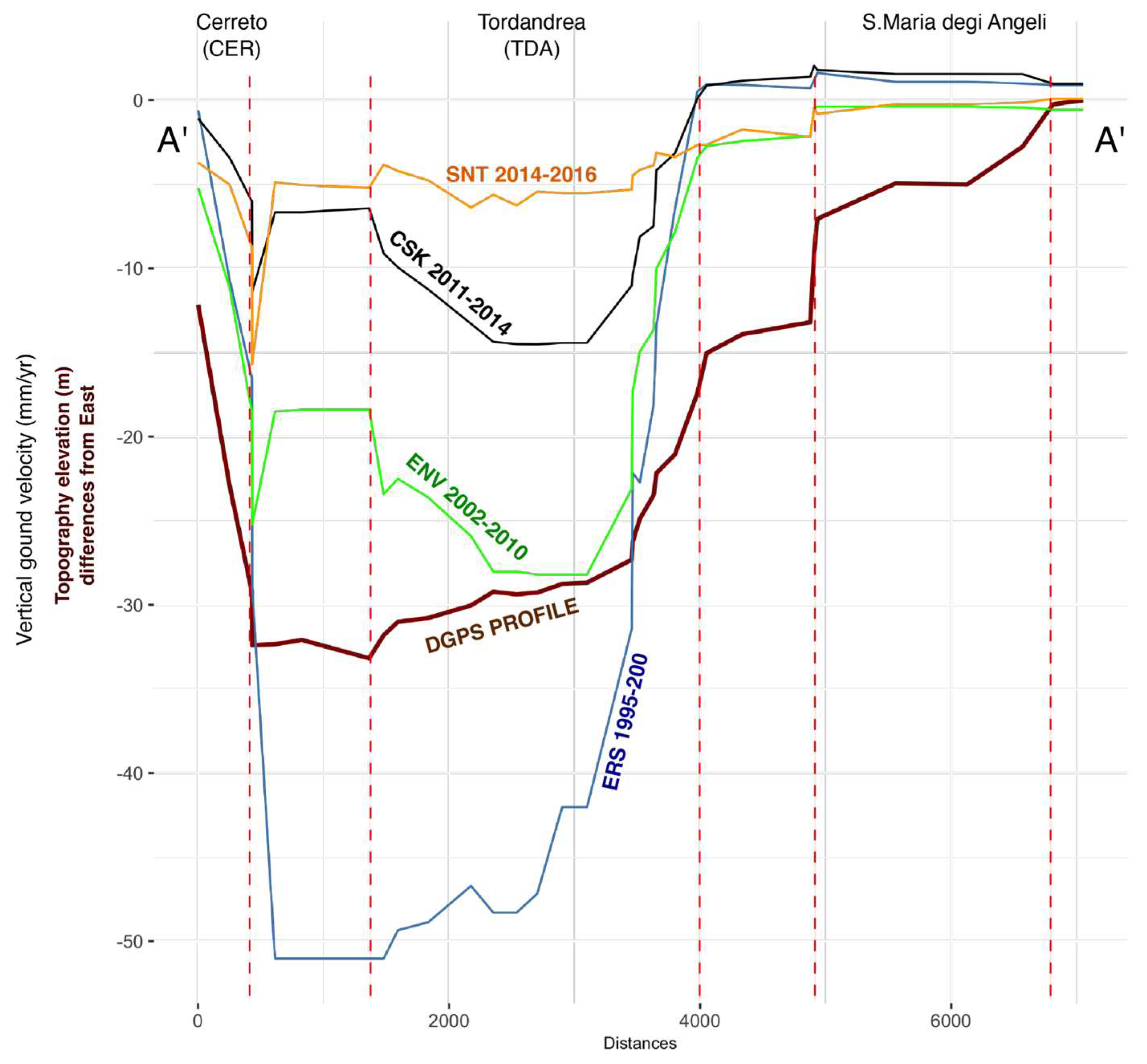
| ERS 1992–2000 | ENV 2002–2010 | CSK 2011–2014 | SNT 2014–2016 | Total Displacement | |||||
|---|---|---|---|---|---|---|---|---|---|
| Years | 8.74 | 7.56 | 2.94 | 1.86 | |||||
| mm yr | mm | mm yr | mm | mm yr | mm | mm yr | mm | mm | |
| TDA | −50.9 | −444.9 | −15.3 | −115.7 | −16.2 | −47.6 | −6.5 | −12.1 | −620.3 |
| CER | −33.2 | −290.2 | −20.1 | −152.0 | −19.7 | −57.9 | −23.0 | −42.8 | −542.8 |
| CAN | −15.9 | −139.0 | −13.4 | −101.3 | −10.7 | −31.5 | −11.3 | −21.0 | −292.7 |
Disclaimer/Publisher’s Note: The statements, opinions and data contained in all publications are solely those of the individual author(s) and contributor(s) and not of MDPI and/or the editor(s). MDPI and/or the editor(s) disclaim responsibility for any injury to people or property resulting from any ideas, methods, instructions or products referred to in the content. |
© 2023 by the authors. Licensee MDPI, Basel, Switzerland. This article is an open access article distributed under the terms and conditions of the Creative Commons Attribution (CC BY) license (https://creativecommons.org/licenses/by/4.0/).
Share and Cite
Brunori, C.A.; Murgia, F. Spatiotemporal Evolution of Ground Subsidence and Extensional Basin Bedrock Organization: An Application of Multitemporal Multi-Satellite SAR Interferometry. Geosciences 2023, 13, 105. https://doi.org/10.3390/geosciences13040105
Brunori CA, Murgia F. Spatiotemporal Evolution of Ground Subsidence and Extensional Basin Bedrock Organization: An Application of Multitemporal Multi-Satellite SAR Interferometry. Geosciences. 2023; 13(4):105. https://doi.org/10.3390/geosciences13040105
Chicago/Turabian StyleBrunori, Carlo Alberto, and Federica Murgia. 2023. "Spatiotemporal Evolution of Ground Subsidence and Extensional Basin Bedrock Organization: An Application of Multitemporal Multi-Satellite SAR Interferometry" Geosciences 13, no. 4: 105. https://doi.org/10.3390/geosciences13040105
APA StyleBrunori, C. A., & Murgia, F. (2023). Spatiotemporal Evolution of Ground Subsidence and Extensional Basin Bedrock Organization: An Application of Multitemporal Multi-Satellite SAR Interferometry. Geosciences, 13(4), 105. https://doi.org/10.3390/geosciences13040105