Abstract
We coupled together high-resolution versions of the ocean–sea ice model NEMO and the ice sheet model BISICLES configured to the Totten Glacier area and ran a series of simulations over the recent past (1995–2014) and under warming conditions (2081–2100; SSP4-4.5) with NEMO in stand-alone mode and with the coupled model to assess the effects of the coupling. During the recent past, the ocean–ice sheet coupling has increased the time-averaged value of the basal melt rate in both the Totten and Moscow University ice shelf cavities by and , respectively. The relationship between the changes in ice shelf thickness and ice shelf basal melt rate suggests that the effect of the coupling is not a linear response to the melt rate but rather a more complex response, driven partly by the dynamical component of the ice sheet model. The response of the ice sheet–ocean coupling due to the ocean warming is a 10% and 3% basal melt rate decrease in the Totten and Moscow University ice shelf cavities, respectively. This indicates that the ocean–ice sheet coupling under climate warming conditions dampens the basal melt rates. Our study highlights the importance of incorporating ocean–ice sheet coupling in climate simulations, even over short time periods.
1. Introduction
The Totten Glacier area, located on the Sabrina coast in East Antarctica, holds the largest potential ice discharge from the East Antarctic ice sheet [1], with an ice volume equivalent to 3.9 m of global sea level rise [2]. With most of its drainage basin grounded well below sea level [3], the Totten Glacier is susceptible to ocean erosion and to ice sheet instability [4].
Recent observations indicate the thinning of the Totten ice shelf (TIS) during the last decade [5], with most of this thinning driven by higher ocean temperatures [6,7]. In addition to this thinning, a 1 to 3 km retreat of the ice shelf grounding line has been detected during the 1996–2013 period [2]. Observations of ice motion over the last few decades have revealed a complex pattern of changes, with the counteraction of increases and decreases in surface ice speed. The glacier exceeded its balance speed in 1989–1996, slowed down in 2000 to bring its ice flux into balance with accumulation, and then accelerated until 2007, and its speed remained constant thereafter [7,8]. As for the ice thinning, there is a strong linkage between the ice dynamics and the ocean temperature [7]. Several studies reported the presence of warm, salty modified Circumpolar Deep Water (mCDW) in the bottom layer of the continental shelf near the TIS cavity, which drives rapid basal melt [9,10,11,12,13]. Other studies have also investigated the effect of the Dalton polynya [5,9], the wind [14], and the ocean intrinsic variability [15] on the TIS basal melt rate.
The ocean can induce modifications in continental ice sheets through changes at the ocean–ice shelf interface [16]. As the ice shelf controls the distribution of normal stresses at the grounding line, changes in ice thickness and grounding line reduce the back-stress that the ice shelf exerts on the upstream ice sheet, leading to an acceleration in the grounded ice speed and to enhanced ice discharge, and thus contributes to the global sea level rise [17,18]. In turn, the induced melting results in freshwater injection at depth, known as Ice Shelf Water. This Ice Shelf Water flows upward along the ice shelf base under the influence of buoyancy, friction, and Coriolis forces in the form of a turbulent plume, continually mixing with warmer seawater [19]. The upward motion of the plume induces an inflow of possibly warmer ocean water into the ice shelf cavity, creating more melt. On the other hand, depending on the stratification of the ocean water inside the cavity, the plume may reach a level of neutral buoyancy from which it is no longer driven upward. The subsequent melting, freezing and density-driven plume circulation alter nearby seawater properties [20,21]. Moreover, ice shelf basal melting is sensitive to the ice shelf cavity shape [16,22].
Over the last few years, an increasing number of coupled ocean–ice sheet models have been developed, such as Global Climate Models (GCMs) of intermediate complexity [16,23], state-of-the-art ocean models [24,25,26] and even state-of-the-art GCMs and Regional Climate Models (RCMs) resolving all the climate components, called Earth system models [27,28]. Several studies, with regional coupled ocean–ice sheet models, have investigated the impact of the coupling on various ice shelf cavities. Seroussi et al. [29] used the coupled MITgcm–ISSM model to study the coupling effects on the Thwaites Glacier under present climate conditions. They observed a decrease in basal melt in response to the thinning of the ice shelf, which causes the ice shelf base to rise above the mCDW layers, before the ice starts increasing again (negative feedback loop). Timmermann and Goeller [24] used the coupled FESOM–RIMBAY model in the Filchner-Ronne Glacier area under present climate conditions. They found higher basal melt rates in coupled mode compared to uncoupled mode, under present-day climate conditions. They also found that an increased water column thickness, due to ice thinning, allows for more transport of warm water to the deepest part of the cavity, increases the slope of the ice base and reinforces the strongest melt rates (positive feedback loop). A coupled ocean–ice sheet study in the TIS area has already been conducted by Pelle et al. [25], using the coupled MITgcm–ISSM model, where they found a 56% increase in TIS melt in a warming climate scenario compared to a control run, and a widespread grounding line retreat along the TIS eastern grounding zone.
Nevertheless, all these studies hold some limitations, such as the absence of tides in all models, which might underestimate the ice shelf basal melt rates as described in Huot et al. [30], or such as constant temperature and salt exchange coefficients in the basal melt rate formulation in Seroussi et al. [29], which should be velocity-dependent following Jenkins et al. [31]. Moreover, these studies use ocean–ice sheet models with relatively coarse horizontal resolutions of the model ocean components (4 km in Pelle et al. [25] and from 1 km at the grounding line to 16 km at the ice shelf front in Timmermann and Goeller [24]), thus not allowing them to resolve eddies, which play a crucial role in controlling the flow across the continental shelf and in the vicinity of grounded zones, or the relatively coarse horizontal resolution of the ice sheet model components (10 km in Timmermann and Goeller [24], from 500 m to 15 km in Seroussi et al. [29] and from 1 km to 20 km in Pelle et al. [25]).
As these ice shelf–ocean interactions may lead to drastic changes in the Totten ice sheet’s stability in the future, it is essential to properly and explicitly resolve these ocean–ice stream interactions, with the evolving grounding line position and ice shelf thickness, in a coupled ocean–ice sheet model framework. Furthermore, in order to adequately resolve the ice–ocean interactions, such a framework must include a high-resolution ocean model capable of partially resolving eddies, velocity-dependent heat and salt exchange coefficients at the ice–ocean interface, an explicit representation of fast ice and the representation of grounded icebergs. The goal of the present study is twofold. Firstly, we aim to model the ocean–ice sheet interactions in the Totten Glacier area and study the effects of the coupling on the ice shelf cavities. Secondly, we aim to assess the response of the coupling to sudden warming. To do so, we couple high-resolution, regional configurations of the ocean–sea ice model NEMO3.6-LIM3 (resolution of approximately 2 km) and the ice sheet model BISICLES (500 m resolution for the fast-flowing ice). Both regional configurations cover the Totten Glacier area in East Antarctica. Then, we compare coupled and ocean stand-alone simulations over the years 1995–2014 and with EC-Earth3 anomalies (2081–2100 [32]) applied at the atmospheric and oceanic forcings of the ocean–sea ice model.
This manuscript is organised as follows. The models, regional configurations, model initialization, coupling interface and experimental design are detailed in Section 2. We analyse the effects of the coupling on the ice shelf cavities and on the ocean and sea ice properties, and the response of the coupling to a sudden warming, in Section 3. Conclusions are finally given in Section 4.
2. Materials and Methods
2.1. Ice Flow Model: BISICLES
Changes in land ice and ice shelves are simulated by the ice sheet model BISICLES [33], a finite-volume model with vertically integrated ice flow based on the hybrid approach of Schoof and Hindmarsh [34] to include membrane stresses. The BISICLES temporal and spatial adaptive mesh refinement is set between 4 km in the slow-moving regions and up to 500 m resolution around the grounding line and fast-flowing areas, where membrane stresses are important. Time steps are adapted automatically to satisfy the Courant–Friedrichs–Lewy condition. At each time step, the ice velocity, surface and base elevation and grounding line position are updated. Basal sliding is based on a Coulomb-limited sliding law after Tsai et al. [35]: with the basal shear stress, = 0.5, N the effective pressure at the bed, C the spatial sliding law coefficient, m = 1/3, and the basal velocity. Throughout the simulation, the ice front position is kept fixed, filling ice-free areas with a minimum ice thickness of 11 m to avoid changing the open ocean area in NEMO, while keeping the buttressing effect of the ice shelf itself low. Basal melt is applied solely on fully floating grid cells, and partial melting underneath grounded grid cells is avoided [36].
The BISICLES Configuration
The ice domain covers the Aurora basin, including the catchments of the Totten and Moscow University ice shelves [37] that are defined by surface slopes from Ice, Cloud and Land Elevation satellite (ICESat) data [38]. Bathymetry, bedrock and ice surface elevation are provided by Bedmachine v.2 [3,39]. For the model initialisation, we first estimate the basal friction and ice stiffness coefficients by solving an inverse problem following MacAyeal [40] and Morlighem et al. [41]. The inversion aims to minimise mismatch between modeled and observed ice surface velocities [42,43], using a conjugate gradient method. Given the estimated coefficients, the ice sheet model is run for 12 years to minimise model drift while keeping the ice thickness as close to present-day observations (Bedmachine v.2) as possible. During the 12-year relaxation simulation, the model is forced by the constant 1995–2014 mean surface mass balance from the regional atmospheric model MAR (Modèle Atmosphérique Régional) at 10 km resolution [44] and mean NEMO melt rates from Van Achter et al. [45] at approximately 2 km resolution around the grounding line. In the coupled simulations, BISICLES is forced by monthly mean ocean melt rates provided by NEMO. To have an estimate for the cells where ice retreats during a coupling window, basal melt rates from NEMO are linearly extrapolated on the 500 m grid to cover also grounding line and first grounded elements. Since the focus of this study is the effects of ice–ocean interactions, the surface mass balance is kept constant beyond the initialisation.
2.2. Ocean and Sea Ice Model: NEMO3.6-LIM3
We use a regional East Antarctic configuration of the NEMO model (Nucleus for European Modelling of the Ocean, [46]) to simulate the ocean–sea ice system. NEMO includes the ocean model OPA (Océan Parallélisé), which is coupled with the Louvain–la Neuve sea ice model (LIM3, [47,48]). This model version, hereafter referred to as NEMO, has been frequently used to study both the whole Southern Ocean, e.g., [28,49,50], and specific Antarctic sectors, e.g., [30,51,52]. The numerical discretisation relies on a C grid [53] and is based upon primitive equations, assuming hydrostatic balance and using the Boussinesq approximation [54]. The vertical discretisation relies on the so-called coordinate, with varying cell thicknesses on the full water column [55]. The vertical mixing is based on a turbulent kinetic energy (TKE) scheme [56,57,58]. In our setting, ocean convection is represented through enhancing the vertical diffusivity to 20 m s in case of an unstable water column. The drag coefficient is set to 7.1 × 10 at the sea ice–ocean interface and 2 × 10 at the sea ice–atmosphere one [59]. The sea ice model relies on an elastic–viscous–plastic (EVP) rheology formulated on a C grid [60], and uses a five-category subgrid-scale distribution of sea ice thickness [61].
The Antarctic ice shelf cavities are opened to the ocean circulation, with explicit ocean–ice shelf interactions [62]. The heat and mass fluxes associated with the melt or freezing are determined by the three-equation formulation of Jenkins [63]. The transfer coefficients for both heat () and salt () between the ocean and ice shelves are velocity-dependent [64]: . The friction velocity is given by and constant values of and taken from Jourdain et al. [51] are used ( and for temperature and salinity, respectively), = is the ocean–ice sheet drag coefficient and is the ocean velocity in the top mixed layer, which is either the top 30 m of the water column or the top model layer (if thicker than 30 m) [65].
The Totten24 Model Configuration
The NEMO Totten24 setup is similar to the configuration used in Van Achter et al. [52] and Van Achter et al. [45]. The ocean grid is a 1/24 refinement (less than 2 km grid spacing) of the eORCA1 tripolar grid, centered on the continental shelf in front of the TIS, East Antarctica, and covering an area between 108–129 E and 63–68 S (Figure 1). The vertical discretisation includes 75 levels, with increasing thickness from ∼1 m at the surface to ∼200 m at depth. Partial cells are used for a better representation of the seafloor and the ice shelf base [66]. The OPA and LIM time steps are 150 s and 900 s, respectively. The ocean layer directly underneath the ice shelf base varies between 30 m near the cavity front and 80 m in the center of the cavity. The bathymetry dataset comes from the NASA MEaSUREs program (BedMachine Antarctica v2, [3]), which contains a bathymetry map of Antarctica based on mass conservation, streamline diffusion and other methods [3]. The initial ice shelf thickness for the ocean model is the relaxed geometry obtained after a 12-year relaxation simulation as described in Section 2.1. The Antarctic surface continental mask is constant time-wise.
At the lateral open-ocean boundaries, NEMO is driven using outputs from a 1979–2014 simulation with an eORCA025 (1/4) NEMO configuration covering the whole Southern Ocean [28] (hereafter referred to as PARASO). PARASO was chosen over reanalyses such as GLORYS12v1 due to its much better representation of ocean temperatures over the continental shelf, which compares well with observations from Rintoul et al. [10]. In order to correct a fresh bias present in PARASO, the ocean salinity lateral boundary condition is uniformly increased by 0.25 g kg. The model is forced daily at the west, north and east boundaries, with SSH, temperatures, salinities, ocean velocities, sea ice concentrations, sea ice thicknesses and snow thicknesses over sea ice. A flow relaxation scheme [67] is applied at the lateral boundaries to the three-dimensional ocean variables and two-dimensional sea ice variables. To allow gravity waves generated internally to exit the model boundaries, a Flather radiation scheme [68] is used at the lateral boundary conditions for barotropic velocities and sea surface elevation (SSH). Furthermore, the SSH and barotropic velocities from the FES2014 tide model [69] are added to the boundary for the tide components K1, K2, M2, P1, O1, S2, 2N2, Mm, M4, Mf, Mtm, MU2, N2, NU2, Q1, S1, L2 and T2, as in Maraldi et al. [70], Jourdain et al. [71] and Huot et al. [30]. Surface boundary fluxes are computed using the CORE bulk formula [72], with atmosphere input coming from ERA5 [73]. No surface salinity restoring is applied.
While the iceberg calving is not dynamically simulated by the model, grounded icebergs are extracted from the remotely sensed mosaic ‘RAMP AMM-1 SAR Image Mosaic of Antarctica, Version 2’ [74] and incorporated into the model as follows: a model cell is imposed as a grounded iceberg (bathymetry value is set to zero) when the cumulative area of all observed icebergs within the cell reaches 2 km. Then, to avoid creating iceberg walls and to ensure regular oceanic circulation, we filter the icebergs to avoid prescribing neighbouring iceberg grid cells. Finally, only the icebergs located in oceanic areas shallower than 450 m are kept. There is no freshwater injection related to the icebergs melting in the model. A fast ice representation is included through the combination of the effect of grounded icebergs with a sea ice tensile strength parameterisation [52]. The EVP rheology of the sea ice is modified to include both isotropic and uniaxial tensile strength based on the tensile strength parameterisation of Lemieux et al. [75]. The eccentricity of the elliptical yield curve and the isotropic tensile strength parameter are set to 1.2 and 0.2, respectively. The number of sub-iterations of the EVP scheme is set to 720 to solve the momentum and the stress equations.

Figure 1.
Model bathymetry and domain. The contour interval is 50 m up to 500 m depth and 500 m up to 4500 m depth. Ice shelf cavities are surrounded by a thick black line. The 0.75 fast ice observed frequency from [76] is shown by the shaded gray areas. The inset (top left) shows Antarctica with the model domain denoted by the grey area (ice sheet model domain) and by the red rectangle (ocean model domain).

2.3. Initialisation and Coupling Interface
For the ocean–ice sheet coupled and ocean stand-alone simulations, the NEMO model is initialised from a 2-year spin-up run performed with NEMO stand-alone, using forcings corresponding to the years 1993 and 1994. This spin-up is started from a 20-year climatology of a 1995–2014 NEMO stand-alone run, which is long enough to reach equilibrium in the ice shelf cavities [45]. The 20-year climatology of the 1995–2014 NEMO stand-alone run is used to provide an average basal melt rate distribution that is later applied in a BISICLES stand-alone relaxed run (described in Section 2.1). This run is performed to generate the initial geometry that will later serve as an initial condition for NEMO for coupled and stand-alone simulations.
The coupling interface between NEMO and BISICLES is based on the coupling interface between NEMO and the ice sheet model f.ETISh used in PARASO [28], and following Smith et al. [27] for ice sheet geometry changes within NEMO. Both the model initialisation and the coupling procedure, which is an off-line coupling, are summarised in Figure 2. NEMO runs first for a coupling time window (here 3 months), sending monthly time series of ice shelf melt fluxes to BISICLES. While NEMO waits, BISICLES runs for the same time window, forced with the received melt rates as a boundary condition. Afterwards, BISICLES provides NEMO with a new ice shelf geometry. NEMO can then start the next 3-month period with its updated ice shelf geometry. These exchanges between both models are repeated over each coupling window until the end of the coupled simulations. The data are bilinearly interpolated from one grid to the other.
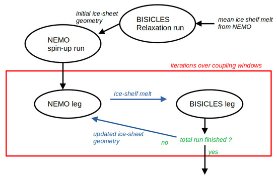
Figure 2.
NEMO–BISICLES coupling procedure. The red box represents the coupling loop. Arrows depict the data exchanged between NEMO and BISICLES.
When NEMO receives the updated ice shelf geometry from BISICLES and before NEMO starts running again, ocean cells may be opened or closed due to the change in ice shelf geometry. To account for these potential changes in geometry, we follow the methodology of Smith et al. [27], as described in Pelletier et al. [28]. For any subshelf ocean cells to open (or close), the following constraints must be met; otherwise, the ocean cell remains closed (or opened). (1) The ice shelf thickness must be greater than 11 m to keep the ice shelf extent constant and (2) the water column thickness must be greater than 50 m. When an ocean cell is opened, the SSH, the temperature and the salinity from neighbouring cells are extrapolated into the newly opened cell [77]. The initial ocean current velocities of the new opened cells are set to zero and a horizontal divergence correction is applied in order to avoid spurious vertical ocean velocities. This approach does not comply with energy and mass conservation, but the amounts are so small that they are negligible for the overall outcome.
When BISICLES receives monthly mean subshelf melt fluxes, mask discrepancies are addressed with a bilinear extrapolation to cover BISICLES ice shelf cavity columns, which correspond to closed columns in NEMO. Ice shelf cavity columns in NEMO, which correspond to grounded ice or open ocean in BISICLES, are disregarded.
2.4. Experimental Design
Our experimental design consists of four 20-year-long simulations (Table 1). The first set of two simulations, devoted to the study of the ocean–ice sheet coupling and its impact on the ice–ocean interactions, is composed of the REF and REF3mcpl simulations, which cover the 1995–2014 period. REF is a NEMO stand-alone simulation and REF3mcpl is a coupled NEMO–BISICLES simulation with a coupling time step of 3 months. Both simulations have the same initial ice shelf thickness, initial ocean conditions and atmospheric and oceanic forcings.

Table 1.
Names and descriptions of the simulations used in this study.
The second set of two simulations, which aims to investigate the response of the ocean–ice sheet coupling to sudden warming, is formed by the WARM and WARM3mcpl simulations. Both simulations correspond to climate conditions that might prevail during the 2081–2100 period. As described in Van Achter et al. [45], annual cycles of the EC-Earth3 climate anomalies from the SSP4-4.5 scenario [32], computed as the differences between 2081–2100 and 1995–2014, have been added to all the fields of the atmospheric and oceanic forcings used for the 1995–2014 period in REF and REF3mcpl. The 2081–2100 simulations use the same initial ice shelf geometry as the 1995–2014 simulations. This experiment is designed to estimate the effects of a present-day versus warmer climate scenario to an ice–ocean coupling setup on a regional scale. Where keeping the same initial ice geometry facilitates the comparison of simulation results, we do not attempt to project the ocean, sea ice, ice sheet and ice shelf characteristics that might prevail by the end of the 21st century. Rather, WARM3mcpl aims at evaluating the response of the NEMO–BISICLES coupling to the sudden warming of ice shelf cavities triggered by changes in atmospheric forcings and oceanic conditions at the boundaries of the domain.
A similar simulation to REF was conducted by Van Achter et al. [52] and evaluated against observations (sea ice concentration, fast ice, sea ice production, sea ice thickness, polynya locations and ocean temperature and salinity distributions) and both REF and WARM simulations are compared in detailed in Van Achter et al. [45].
3. Results
3.1. Ocean–Ice Sheet Coupling Effects on the Ice Shelf Cavities
Time series of area-averaged ice shelf basal melt rates in REF and REF3mcpl (continuous and dotted blue lines in Figure 3) indicate that the NEMO–BISICLES coupling over the years 1995–2014 tends to slightly increase the basal melt rate in the TIS cavity and its neighbouring Moscow University ice shelf (MUIS) cavity. In both cavities, the coupled simulation shows higher basal melt rates with a clear increase after the fifth year of the simulation. The TIS basal melt rates averaged over the years 1995–2014 are 10 ± 1.88 and 10.68 ± 1.95 m year for REF and REF3mcpl, respectively. Likewise, the MUIS basal melt rates are 6.2 ± 2.38 and 7.09 ± 2.58 m year for REF and REF3mcpl, respectively. These simulated basal melt rates are in good agreement with the estimates of Rignot et al. [78], namely 10.74 ± 0.7 m year for TIS and 4.7 ± 0.8 m year for MUIS. The basal melt rates in REF3mcpl are increased by 6.7% in TIS and 14.2% in MUIS, and the differences between the two experiments are much smaller than the simulated interannual melt rate variability (SD in REF: 3.56 m year in TIS and 5.68 m year in MUIS), which is partly driven by the oceanic lateral boundary conditions (correlation of 0.5 between the ocean temperature at the ocean boundaries and the MUIS basal melt rate). The effect of the coupling on the basal melt rate is not constant over time and fluctuates between +0.5 and +2 m year and is related to the interannual variability of the basal melt rate: a high melting year is related to a stronger effect of the coupling on the basal melt rate and vice versa.
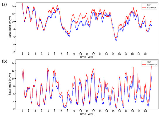
Figure 3.
Area-averaged basal melt rate in the TIS (a) and MUIS (b) cavities for the REF (blue) and REF3mcpl (red) simulations over the 1995–2014 period. The TIS mean basal melt rate amounts to 10 ± 1.88 m year for REF and 10.68 ± 1.95 m year for REF3mcpl. The MUIS mean basal melt rate amounts to 6.2 ± 2.38 m year for REF and 7.09 ± 2.58 m year for REF3mcpl.
The spatial distributions of the mean basal melt rates for REF and REF3mcpl are displayed in Figure 4a,b, respectively. Maximum melt rates in both simulations are around 60 m year and occur in the deepest part of the cavity near the grounding line, where the ice base reaches 1100 and 1300 m below sea level, and the freezing point is approximately 1 C below the surface freezing point. Differences between REF3mcpl and REF (Figure 4c) show that the melt rates below the TIS in the coupled run are decreased along the eastern flank of the cavity and increased along the western flank. Moreover, in both the TIS and MUIS cavities, high values of the basal melt rate in REF are found in both the middle and the bottom of the cavity in REF, while, in REF3mcpl, they are located only in the bottom of the cavity. Furthermore, part of the basal melt rate heterogeneity in REF is smoothed out in REF3mcpl, which exhibits a relatively more homogeneous spatial distribution of the basal melt rate compared to REF.
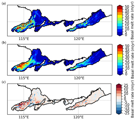
Figure 4.
Spatial distributions of the mean basal melt rate for the REF (a) and REF3mcpl (b) simulations over the 1995–2014 period. Differences in basal melt rate between REF3mcpl and REF, averaged over the 1995–2014 period (c).
The impacts of the coupling on the ocean temperature and velocity at the ice–ocean interface (first ocean layer beneath the ice shelves) are depicted in Figure 5 and Figure 6, respectively. The ocean temperature at the ice–ocean interface is decreased in the coupled simulation in all cavities near the cavity fronts, down to −0.2 C. On the other hand, the ocean temperature is increased by more than 0.1 C near the bottom of the cavities. The TIS shows a higher mean ocean temperature than the MUIS, with values reaching −0.9 C at the bottom of the TIS cavity and −1.8 C in the MUIS cavity (see Figure 5a). Despite their differences in mean ocean temperature, both TIS and MUIS cavities exhibit the same ocean warming at the ice–ocean interface in the coupled simulation compared to the fixed ice shelf geometry simulation (see Figure 5b). The cooling, however, is much larger at the TIS cavity front than at the MUIS cavity front. The differences in cooling between both fronts of the TIS and MUIS cavities might partly be related to the larger amount of cold melt water released by the MUIS cavity, which cools down the ocean (even at the surface, as shown in Figure 5b) on the western side of the MUIS in REF3mcpl compared to REF. Cold Ice Shelf Water (water colder than −1.92 C) is found in the MUIS cavity but does not exit the cavity, as it is warmed up along its way towards the ice shelf front.
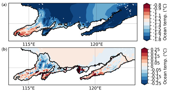
Figure 5.
Mean ocean temperature at the ice–ocean interface in REF (a). Differences in ocean temperature at the ice–ocean interface between REF3mcpl and REF (b), averaged over 1995–2014.
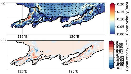
Figure 6.
Mean ocean current velocity at the ice–ocean interface in REF (a). Differences in ocean current speed at the ice–ocean interface between REF3mcpl and REF (b), averaged over 1995–2014.
The ocean current speeds at the ice–ocean interface are intensified in the coupled simulation compared to the fixed ice shelf geometry simulation. The mean ocean velocities in REF at the ice–ocean interface are characterised in both the TIS and MUIS cavities by a clockwise circulation, with a slow entering current along the eastern side of the cavities and a faster (up to 0.2 m s) outgoing current along the western side (Figure 6a). In the coupled run, the ocean speeds at the ice–ocean interface are enhanced up to 0.1 m s, mostly in areas where the ice shelf thickness thinned during the coupling (as on the western side of the TIS cavity). Other regions display a slowdown of the ocean currents due to the change in ice shelf thickness, as on the eastern side of the TIS cavity where the ice shelf has thickened.
Vertical sections of ocean temperature, salinity and meridional velocity across the TIS cavity are shown in Figure A3 and Figure A4 (in Appendix A). The bottom of the cavity is filled with colder (−0.1 C) and fresher waters (−0.01 g kg) in REF3mcpl, which is the opposite of what is found at the ice–ocean interface (warmer and saltier in REF3mcpl). The ocean stratification seems to be similar in both REF3mcpl and REF. The temperature and salinity effects on the stratification at the ice–ocean interface are opposite (higher temperature and higher salinity in REF3mcpl) and may explain the lack of changes in stratification inside the cavity. The meridional circulation inside the TIS cavity shows, at the ice–ocean interface, a steady rising current from the bottom to the front of the cavity. This plume circulation exhibits the same intensity in both simulations, except where the ice shelf thickness is modified in REF3mcpl, where the plume circulation is enhanced.
The changes in the ice shelf draft (ice shelf thickness below sea level) and grounding line position after 20 years of the coupled simulation are illustrated in Figure 7a,b, respectively. The TIS experiences a thickening near the front of the cavity, with an ice gain reaching more than 150 m. Deeper into the cavity, the ice thickness is decreased by more than 200 m. As illustrated in Figure A2, both the thinning and thickening of the ice shelf have smoothed the ice–ocean interface. The MUIS exhibits a more heterogeneous change in thickness near its cavity front, and a large ice thickness increase near the bottom of its cavity. There is no change in the grounding line position in the two main ice shelf cavities. Nonetheless, there is a grounding line migration around 119 E, which closes half of a small ice shelf cavity between TIS and MUIS, and is explained by the lower ocean temperature at the ice–ocean interface (−0.1 C) due to the increased basal melt rate in its neighbouring MUIS cavity in REF3mcpl.
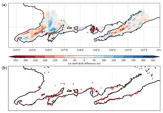
Figure 7.
(a) Changes in ice shelf draft after 20 years in REF3mcpl. The loss of ice is in red and the gain of ice in blue. The changes are relative to the initial ice shelf draft depth. (b) Changes in grounding line position throughout the coupled run. The black and red lines are the initial and final grounding line positions, respectively.
A recent study by Li et al. [79] observed a grounding line retreat over the 1996–2020 period of 9.37–13.85 km at the eastern and western flanks of the MUIS cavity and of 5.95 and 3.51 km at the TIS cavity. Even the maximum grounding line retreat reaches less than 1 km year, which may explain why our 2 km ocean horizontal resolution does not reproduce this grounding line retreat in REF3mcpl. Moreover, the threshold value of a minimum of 50 m water column thickness for a cell to become ungrounded may also limit the grounding line retreat, and the basal melt rates along the grounded zone are relatively low (less than 15 m year) and may result in underestimated grounding line retreat in REF3mcpl.
Cross-sections of the ice shelf base elevation for both the TIS and MUIS are presented in Figure A2a,c (in Appendix A). In the TIS zone, the ice shelf base is unchanged in REF3mcpl from the grounding line until 67.1 S, where the changes in ice shelf thickness increase the slope of the ice shelf base, which may reinforce the plume circulation and locally enhance the basal melt. Further north, around 67 S, the slope of the ice shelf base in REF3mcpl is strongly decreased compared to the one in REF, which decreases the basal melt rates in REF3mcpl around this latitude, as shown in Figure 4. Near the ice shelf front, the ice shelf is thickened in REF3mcpl, which should enhance the basal melt due to the increased freezing temperature. On the other hand, the slope of the ice shelf base is decreased and may explain the locally slower plume circulation and subsequent lower basal melt rates in REF3mcpl near the TIS front. The year-to-year changes in ice shelf base depth (each line is a different year in Figure A2a,c) indicate that the thinning of TIS has reached its equilibrium after 5 years (changes in ice shelf base depth between year 5 and 20 are very small). On the other hand, the ice thickening at the TIS front is not yet at equilibrium (ice shelf base depths between year 15 and 20 are not yet overlapping). The changes in ice shelf base elevation for the MUIS are less significant.
The next step is to investigate the origin of the changes in basal melt rates between REF3mcpl and REF. Figure 8a indicates that the link between the changes in ocean temperature and the changes in basal melt rate is weak. Their linear regression shows a relationship between a higher ocean temperature at the ice–ocean interface and higher basal melt and vice versa, but the R value is low (0.129). On the other hand, there is a clear link between the changes in ocean current speed at the ice–ocean interface and the changes in basal melt rate (Figure 8b). The linear regression reveals, with an R value of 0.573, that higher basal melt rates in REF3mcpl compared to REF are generally related to increased ocean current speeds in REF3mcpl compared to REF, and the same is true for lower basal melt rates and decreased ocean current speeds. The relationship between changes in ice shelf base slope and basal melt rates, shown in Figure A1, indicates that the basal melt rates in REF3mcpl are related to steeper slopes compared to the basal melt rates in REF.
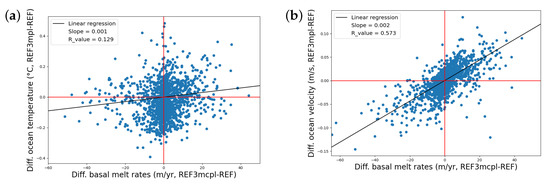
Figure 8.
Scatter plots of the differences in basal melt rate between REF3mcpl and REF as function of the differences in ocean temperature (a) and the differences in ocean current speed (b). All differences between REF3mcpl and REF are computed over the 20-year simulation period. Both the ocean temperature and speed are taken in the first ocean layer beneath the ice.
Areas of changes in mean basal melt rate in the TIS cavity related to changes in ocean temperature and current speed are highlighted in Figure 9. Regions of increased basal melt rate linked to higher ocean temperatures are few, and most of them are limited to the smaller cavity located on the eastern side of the main cavity. On the other hand, the areas of increased basal melt rate related to a larger ocean current speed cover a large part of the cavity—in particular, the western side of the cavity, where the higher basal melt rate increase occurs (see Figure 4c). Regions of decreased basal melt rate in REF3mcpl associated with a lower ocean temperature are also related to slower ocean currents, and are located near the cavity front (see Figure 9c,d). The decreased basal melt rates on the eastern flank of the cavity (see Figure 4c) are partly driven by decreased ocean current speeds (Figure 9d).
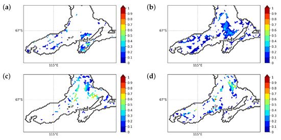
Figure 9.
Locations in the TIS cavity where the mean basal melt rate increases in REF3mcpl compared to REF are related to an increased ocean temperature (a) or to an increased ocean current speed (b). Locations where the mean basal melt rate decreases in REF3mcpl compared to REF are related to a decreased ocean temperature (c) or to a decreased ocean current speed (d). The colour bar represents the normalised distance between each point and the regression line (value close to zero means a strong linear relationship).
Under stable ocean vertical stratification, a reduced ice shelf thickness makes the in situ freezing temperature increase, thus implying a decrease in melt at constant inflow towards the ice shelf cavity. Therefore, with this assumption, the expected coupling response is that a reducing (increasing) ice thickness would eventually reduce (increase) the basal melt rate. Nevertheless, a more complex response is found in REF3mcpl, as revealed by Figure 10a, which shows the link between the 20-year basal melt rates and changes in ice shelf thickness. The scatter plot indicates that there are indeed areas with large values of basal melt rate related to larger ice shelf thicknesses, but there are also regions of lower ice shelf thicknesses caused by larger values of the basal melt rate. Moreover, most areas with a basal melt rate greater than 300 m are mostly related to a decreased ice shelf thickness.
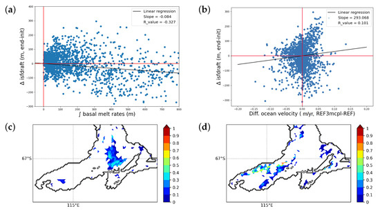
Figure 10.
Scatter plot of the time-integrated basal melt rates and the changes in ice shelf thickness (a). A negative value in ice shelf thickness means a decreased ice thickness. Scatter plot of the differences in ocean current speed as a function of the changes in ice shelf thickness (b). Locations in the TIS cavity where increased ocean current speed is related to an increased ice shelf thickness (c) or to a decreased ice shelf thickness (d). The colour bar represents the normalised distance between each point and the regression line (value close to zero means a strong linear relationship).
Figure 10c suggests no clear link between changes in ocean current speed and changes in ice shelf thickness, with a small R value of 0.101. Areas of accelerated ocean current are found in ice shelf areas that are related to ice thickening as well as ice thinning (see Figure 10b,c). Nevertheless, in areas of high basal melt rates, there is a strong relationship between an increased ocean current speed, increased basal melt rates and reduced ice shelf thickness (Figure A5 in Appendix A). This positive feedback is explained by Timmermann and Goeller [24]. The reduced ice shelf thickness, which means a thicker water column, allows for more transport of warm water to the deepest parts of the cavity and allows for faster ocean currents at the ice–ocean interface. These faster ocean currents then enhance the basal melt rates.
To account for the ice dynamics (up to 2 km year in the fast-flowing parts of the TIS; see Figure 11), the relationship between the divergence of the ice shelf thickness flux and the changes in basal melt rate is shown in Figure 11. The divergence of the ice shelf thickness flux expresses the loss of ice volume related to basal melting while taking into account the loss of ice volume related to horizontal ice transport. The ice shelf thickness flux divergence and the basal melt rate exhibit a strong linear relationship, with higher melt rates related to more ice volume loss (the effects of the coupling on the ice sheet model will be discussed in another study). Figure 10 and Figure 11 suggest that the changes in ice shelf thickness are not the simple integrated response of the changes in basal melt rate (thinner ice implies less melt), but are more complex. On the one hand, a reduced ice thickness may locally raise the basal melt rate. On the other hand, the changes in ice shelf thickness are also driven by the dynamics of the ice sheet. This result highlights the importance and the added value of the ocean–ice sheet coupling.
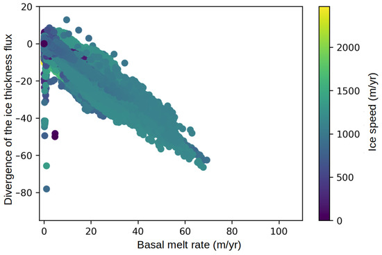
Figure 11.
Scatter plot of the basal melt rate and the divergence of the ice shelf thickness flux in REF3mcpl, averaged over the 20-year simulation. The colour bar indicates the mean ice velocity.
3.2. Ocean–Ice Sheet Coupling Impact on the Ocean Properties and Sea Ice over the Continental Shelf
The impact of the coupling outside of the ice shelf cavities is small. The ocean temperature and salinity properties over the continental shelf in front of the TIS are illustrated in Figure 12a. Due to the overall enhanced basal melt rate in both the TIS and MUIS cavities, the larger amount of cold melt water in REF3mcpl cools down and reduces the salt content of the water masses over the continental shelf. However, the changes are rather small, with temperature differences less than 0.05 C and salinity differences less than 0.01 g kg.
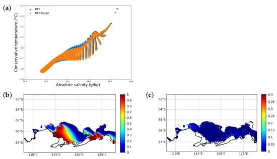
Figure 12.
Temperature–salinity diagram (a) representing the ocean properties over the continental shelf in front of the TIS in REF3mcpl (red) and REF (blue). Fast ice frequency in REF (b), and fast ice frequency differences between REF3mcpl and REF (c). The fast ice and ocean properties are averaged over the 20-year simulations.
The fast ice frequency in REF and its changes compared to REF3mcpl are shown in Figure 12b,c. The frequency differences are close to zero everywhere, except on the western side of the TIS cavity, where the differences in fast ice frequency reach 0.2. This indicates that the lower ocean temperatures in front of the TIS cavity, due to the coupling, lead to up to two additional months of fast ice per year. Nevertheless, these results must be interpreted with caution as the close location of the oceanic boundary conditions must certainly reduce the effects of the coupling on the open ocean.
3.3. Sensitivity of the Ocean–Ice Sheet Coupling Response to Sudden Warming
The ocean and sea ice changes in WARM compared to REF are similar to the ones documented in Van Achter et al. [45]. Here, we focus on the comparison between WARM and WARM3mcpl. The area-averaged basal melt rates for both WARM and WARM3mcpl are presented in Figure 13. The differences in basal melt rate are lower between WARM3mcpl and WARM than in the REF experiments. WARM3mcpl has a lower mean basal melt rate in the TIS cavity by 3.6% and a higher one by 11.6% in the MUIS cavity compared to WARM.
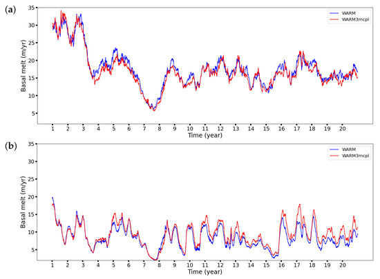
Figure 13.
Area-averaged basal melt rates of the TIS (a) and MUIS (b) cavities for the WARM (blue) and WARM3mcpl (red) simulations over the 1995–2014 period. The TIS mean basal melt rate amounts to 18.63 ± 6.71 m year for WARM and 17.83 ± 7 m year for WARM3mcpl. The MUIS mean basal melt rate amounts to 8.77 ± 3.38 m year for WARM and 9.09 ± 3.46 m year for WARM3mcpl.
REF3mcpl and WARM3mcpl do not start from a balanced coupled state but from the same initial state as REF and WARM for an easier comparison between them. As a consequence, a small drift is seen in REF3mcpl compared to REF due to the coupling. The difference between WARM3mcpl and WARM includes also such a drift, in addition to the different responses of the coupling to the warming. If we assume that the drift in basal melt rate is independent of the initial conditions, it can be evaluated from the difference between REF3mcpl and REF (+6.7% in TIS and +14.2% in MUIS). We can then subtract this drift from the basal melt rate differences between WARM3mcpl and WARM to isolate the changes in the basal melt rate response to the warming associated with the coupling. This leads to a basal melt rate response to the warming of −10% in TIS and −3% in MUIS. Under this hypothesis, the ice sheet coupling reduces the effect of the ocean warming on the basal melt rates in both cavities and can be seen as a negative feedback.
The spatial distributions of the basal melt rate in WARM and WARM3mcpl (see Figure 14) show at the first order the same changes as REF and REF3mcpl (which supports our condition-independent drift hypothesis). The high values of basal melt rate, found in the middle and center of the TIS cavity in WARM, are limited to the bottom of the cavity in WARM3mcpl. Furthermore, the basal melt rates are increased in the western side of the TIS cavity and decreased in its eastern side. Moreover, as in REF3mcpl, the melt rates in WARM3mcpl are smoothed out and differences between WARM3mcpl and WARM can reach up to 30 m year.
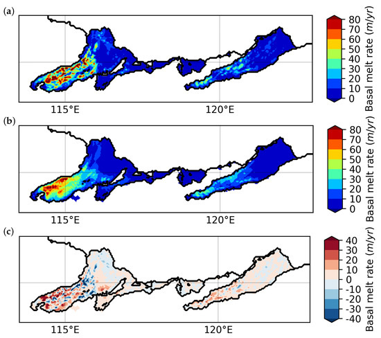
Figure 14.
Spatial distributions of the mean basal melt rate for the WARM (a) and WARM3mcpl (b) simulations over the 2081–2100 period. Differences in basal melt rate between WARM3mcpl and WARM, averaged over the 1995–2014 period (c).
The changes in ice shelf thickness throughout the WARM3mcpl simulation are shown in Figure 15. The MUIS cavity exhibits the same changes in ice shelf thickness as in REF3mcpl (see Figure 7a), which could be explained by the limited effect of the warmer oceanic conditions in the MUIS cavity [45]. In the TIS cavity, most of the areas of ice thickening are the same as in REF3mcpl, with the same magnitude of change (up to 150 m of ice), except the one at the bottom of the cavity, which is no longer thickening in WARM3mcpl. On the other hand, the areas of ice thinning in WARM3mcpl in TIS are almost identical to those in REF3mcpl but experience larger ice losses (up to 350 m of ice loss). Cross-sections of the ice shelf base elevation for both TIS and MUIS are shown in Figure A2b,d (in Appendix A). The changes in ice shelf thickness for the TIS increase the slope of the base of the ice shelf, from the grounding line until 67.1 S. In the middle of the TIS cavity, the ice shelf base slope is strongly decreased, which may explain the lower basal melt rates (in addition to the thinned ice shelf). The year-to-year changes in ice shelf base elevation indicate that the ice thinning of the TIS has not yet reached its equilibrium at the end of WARM3mcpl, as the the ice shelf thickness still shows changes after 20 years of simulation. On the other hand, the ice thickening near the cavity front seems to have reached its equilibrium, as years 6 to 20 are overlapping. As in REF3mcpl, the changes in ice shelf thickness in MUIS are small.
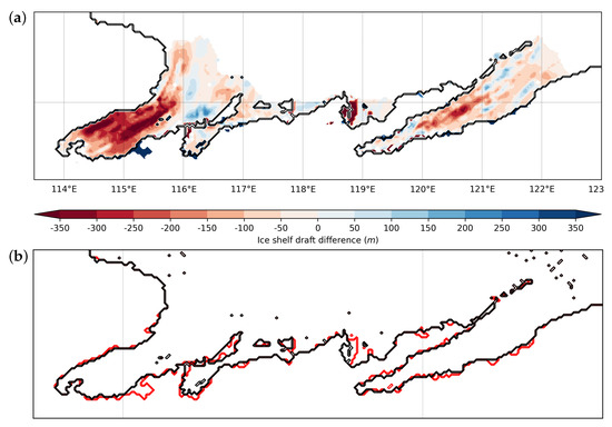
Figure 15.
(a) Changes in ice shelf draft after 20 years in WARM3mcpl. The loss of ice is in red and gain of ice in blue. The changes are relative to the initial ice shelf draft depth. (b) Changes in grounding line position throughout the coupled run. The black and red lines are the initial and final grounding line positions, respectively.
The changes in grounding line position after 20 years of simulation exhibit a similar behaviour in WARM3mcpl as in REF3mcpl (see Figure 15b), except on the eastern side of the TIS cavity, where the grounding line has retreated. This retreat, which occurs after 19 years of coupling, is found around the same location where Pelle et al. [25] simulated grounding line retreat in the TIS cavity under warm climate conditions.
The negative feedback associated with the ice sheet coupling, which reduces the effect of the ocean warming on the basal melt rate, can be explained by the changes in basal melt rate present in the center of the cavity. In this zone, where high melt rates are observed in WARM, melt rates are decreased in WARM3mcpl. As illustrated in Figure A8 (in Appendix A), at these locations, the ice shelf starts to thin at the beginning of WARM3mcpl (from 800 to 500 m of ice) but stabilises after 3 years. As described in Seroussi et al. [29], a thinner ice shelf decreases the pressure at the ice–ocean interface, which results in a rise in the in situ freezing temperature that, at some point, becomes larger than the ocean temperature and decreases the basal melt rates (the changes in the in situ ocean salinity are too small to induce a significant effect on the freezing point temperature in our experiments).
4. Discussion and Conclusions
The first aim of this study was to analyse the impact of the ocean–ice sheet coupling in the Totten Glacier area. To reach this goal, we coupled together high-resolution versions of the ocean–sea ice model NEMO and the ice sheet model BISICLES configured to this region and ran two simulations over the 1995–2014 period: one with NEMO in stand-alone mode and another one with the coupled NEMO-BISICLES model. These simulations revealed that the basal melt rates are increased with the coupling by 6.7% in the TIS cavity and by 14.2% in the MUIS cavity. In addition, the coupling leads to the smoothing of the basal melt rate’s spatial distribution. The changes in basal melt rate due to the coupling show a strong linear relationship with the changes in ocean current speed, with faster ocean currents generating more basal melt and slower ocean currents inducing less melt. The changes in basal melt rate are not linearly related to the changes in ocean temperature. The increased basal melt rates in the TIS are largely caused by increased ocean current speeds at the ice–ocean interface, both in the center and near the bottom of the cavity. On the other hand, the decreased basal melt rates in the TIS cavity, mostly near the cavity front, originate from both lower ocean temperatures and slower ocean currents. The relationship between changes in ocean current speed at the ice–ocean interface and the changes in ice shelf thickness is not clear, as faster ocean currents are found in both areas of thicker and thinner ice shelves. However, increased ocean velocities are often found in areas of high basal melt rates and a thinned ice shelf. This is explained by the thicker water column and by the steeper slope at the ice shelf base, allowing faster ocean currents and enhancing the basal melting (positive feedback).
A nonlinear link is found between the total basal melt rate and changes in ice shelf thickness, with a large number of positive values of the total basal melt rate related to a thicker ice shelf. Nevertheless, most areas with a total basal melt rate higher than 300 m are related to a thinner ice shelf. This suggests that the changes in ice shelf thickness are not a linear response to the melt rate but rather a more complex response, driven by both the basal melt rates and by the dynamics of the ice sheet.
An effect of the ocean–ice sheet coupling outside of the ice shelf cavities is detected in the ocean properties over the continental shelf, with slightly cooler and fresher water masses near the cavities’ outflow. There is also a fast ice frequency increase (up to 2 more months of fast ice per year in some areas), but these changes are small and limited to the western side of the main cavities.
The second goal of this study was to investigate the sensitivity of the response of the ocean–ice sheet coupling to sudden warming. To do so, we ran two additional simulations with EC-Earth3 anomalies (2081–2100) added to the oceanic and atmospheric forcings of the NEMO model. The area-averaged basal melt rates in the simulation conducted with the coupled model are decreased by 3.6% in the TIS cavity and increased by 11.6% in the MUIS cavity compared to the simulation carried out with NEMO in stand-alone mode. Considering that the ice shelf melt rate drift due to the coupling in the 2081–2100 simulation is the same as the one in the 1995–2014 simulation, we can remove the effect of this drift and obtain the response of the ocean–ice sheet coupling due to the ocean warming, which corresponds to a 10% and 3% basal melt rate decrease in the TIS and MUIS cavities, respectively. This suggests that the coupling tends to attenuate the basal melt rates under warmer ocean conditions. This negative feedback is explained by the ice shelf thinning that raises the in situ freezing temperature at the ice–ocean interface and decreases the basal melt rates in the ocean–ice sheet coupled simulation compared to the ocean stand-alone run.
One limitation of our work is the short period of our simulations. As described in Goldberg et al. [16], the ocean circulation usually takes a couple of years to adjust to changes in ice shelf cavity and the glacier flow takes decades to adapt to changes in melt rates. Thus, longer simulations, as in Siahaan et al. [80] or Timmermann and Goeller [24], would allow us to better understand which part of the ice shelf thickness change is due to the initialisation or to the dynamical component of the ice sheet model, which has a slower response than the ocean. Another limitation of our model is its difficulty in representing the grounding line movements, which are underestimated in REF3mcpl in the main ice shelf cavities. Additional experiments should be conducted to study how the grounding line retreats could be better represented. Another perspective is to analyse the effect of tidal representation and high horizontal resolution on ice sheet–ocean coupling, which would help in determining the model developments that require prioritisation for ice sheet–ocean coupling in GCMs.
Although the effect of the coupling on the basal melt rate is smaller than the basal melt rate’s interannual variability, this study showed the importance of ocean–ice sheet coupling, even over a short time period such as 20 years. The coupling impact outside of the ice shelf cavities is small, but other larger ice shelves may have a greater influence on the ocean properties in coupled mode. Finally, our simulations with the coupled model indicate that ocean stand-alone simulations with fixed ice shelf geometry may overestimate the future changes in basal melt rates, at least in some regions. This highlights the importance of using coupled models for century-scale simulations of the Antarctic coastal climate or for global sea level projections.
Author Contributions
Formal analysis, G.V.A.; Software, G.V.A., C.P. and K.H.; Supervision, T.F., H.G. and F.P.; Writing—original draft, G.V.A.; Writing—review and editing, T.F., H.G., C.P., K.H. and F.P. All authors have read and agreed to the published version of the manuscript.
Funding
This research has been supported by the Fonds De La Recherche Scientifique—FNRS (grant no. O0100718F).
Data Availability Statement
The bathymetry and ice shelf draft datasets are accessible at https://doi.org/10.5067/GMEVBWFLWA7X [39,41]. The iceberg dataset can be accessed at https://doi.org/10.4225/15/574BD37A1C6B4 [27].
Acknowledgments
This work was supported by the PARAMOUR project “Decadal predictability and variability of polar climate: the role of atmosphere-ocean-cryosphere multiscale interactions”, supported by the Fonds de la Recherche Scientifique—FNRS and the FWO under the Excellence of Science (EOS) programme (grant no. O0100718F, EOS ID no. 30454083). Hugues Goosse is a research director with the F.R.S-FNRS (Belgium). Computational resources have been provided by the supercomputing facilities of the Université Catholique de Louvain (CISM/UCL) and the Consortium des Equipements de Calcul Intensif en Fédération Wallonie Bruxelles (CECI) funded by the Fond de la Recherche Scientifique de Belgique, Belgium (F.R.S.-FNRS), under convention 2.5020.11. The present research benefited from computational resources made available on the Tier-1 supercomputer of the Fédération Wallonie-Bruxelles infrastructure funded by the Walloon Region under the grant agreement n1117545.
Conflicts of Interest
The authors declare no conflict of interest.
Abbreviations
The following abbreviations are used in this manuscript:
| BISICLES | Berkeley Ice Sheet Initiative for Climate at Extreme Scales model |
| ERA5 | fifth-generation ECMWF atmospheric reanalysis |
| EVP | elastic–viscous–plastic |
| FESOM | Finite-Element volumE Sea ice–Ocean Model |
| GCMs | Global Climate Models |
| LIM | Louvain–la Neuve sea ice model |
| MAR | Modèle Atmosphérique Régional |
| mCDW | modified Circumpolar Deep Water |
| MITgcm | Massachusetts Institute of Technology general circulation model |
| MUIS | Moscow University Ice Shelf |
| OPA | Océan Parallélisé |
| RCMs | Regional Climate Models |
| RIMBAY | Revised Ice Model Based on frAnk pattYn |
| SSH | sea surface elevation |
| TIS | Totten Ice Shelf |
| TKE | Turbulent Kinetic Energy |
Appendix A

Figure A1.
Scatter plot of the mean basal melt rates and the local slope of the ice shelf base. The local slope is computed as the sum of the zonal and meridional slopes and a positive value represents an upward slope towards the north or east.


Figure A2.
Temporal evolutions of the TIS (a,b) and MUIS (c,d) base elevation for REF3mcpl (a–c) and WARM3mcpl (b–d). Black lines denote the initial ice shelf base elevation, the dotted black lines are the ice shelf base elevation at the end of REF3mcpl and WARM3mcpl. Each colour represents 1 year. The subfigures are the locations of the TIS and MUIS sections.


Figure A3.
Cross-sections in the TIS cavity of ocean temperature for REF3mcpl (a) and REF (c), and of ocean temperature difference between REF3mcpl and REF (e). Cross-sections in the TIS cavity of ocean salinity for REF3mcpl (b) and REF (d), and of ocean salinity difference between REF3mcpl and REF (f). All averaged over the 20-year simulations. The section is shown in (a).


Figure A4.
Cross-sections in the TIS cavity of ocean meridional current speed for REF3mcpl (a) and REF (b), and of ocean meridional current speed difference between REF3mcpl and REF (c). All averaged over the 20-year simulations.


Figure A5.
Time series of the difference in basal melt rate, ocean current speed and ice shelf draft over the 20-year period in REF and REF3mcpl. All time series are averaged only where the mean basal melt rate is higher than 50 m year.


Figure A6.
Cross-sections in the TIS cavity of ocean temperature for WARM3mcpl (a) and WARM (c), and of ocean temperature difference between WARM3mcpl and WARM (e). Cross-sections in the TIS cavity of ocean salinity for WARM3mcpl (b) and WARM (d), and of ocean salinity difference between WARM3mcpl and WARM (f). All averaged over the 20-year simulations. The section is shown in (a).


Figure A7.
Cross-sections in the TIS cavity of ocean meridional current speed for WARM3mcpl (a) and WARM (b), and of ocean meridional current speed difference between WARM3mcpl and WARM (c). All averaged over the 20-year simulations.


Figure A8.
Time series of the difference in basal melt rate, ocean current speed, ocean temperature and ice shelf draft over the 20-year period in WARM and WARM3mcpl. All time series are averaged where the mean basal melt rate is higher than 50 m year in the center of the TIS cavity.

References
- Rignot, E. Changes in ice dynamics and mass balance of the Antarctic ice sheet. Philos. Trans. R. Soc. A Math. Phys. Eng. Sci. 2006, 364, 1637–1655. [Google Scholar] [CrossRef] [PubMed]
- Li, X.; Rignot, E.; Morlighem, M.; Mouginot, J.; Scheuchl, B. Grounding line retreat of Totten Glacier, East Antarctica, 1996 to 2013. Geophys. Res. Lett. 2015, 42, 8049–8056. [Google Scholar] [CrossRef]
- Morlighem, M.; Rignot, E.; Binder, T.; Blankenship, D.; Drews, R.; Eagles, G.; Eisen, O.; Forsberg, R.; Fretwell, P.; Goel, V.; et al. Deep glacial troughs and stabilizing ridges unveiled beneath the margins of the Antarctic ice sheet. Nat. Geosci. 2020, 13, 132–137. [Google Scholar] [CrossRef]
- Sun, S.; Pattyn, F.; Simon, E.G.; Albrecht, T.; Cornford, S.; Calov, R.; Dumas, C.; Gillet-Chaulet, F.; Goelzer, H.; Golledge, N.R.; et al. Antarctic ice sheet response to sudden and sustained ice-shelf collapse (ABUMIP). J. Glaciol. 2020, 66, 891–904. [Google Scholar] [CrossRef]
- Khazendar, A.; Schodlok, M.; Fenty, I.; Ligtenberg, S.; Rignot, E.; van den Broeke, M. Observed thinning of Totten Glacier is linked to coastal polynya variability. Nat. Commun. 2013, 4, 2857. [Google Scholar] [CrossRef] [PubMed]
- Aitken, A.R.A.; Roberts, J.L.; Ommen, T.D.v.; Young, D.A.; Golledge, N.R.; Greenbaum, J.S.; Blankenship, D.D.; Siegert, M.J. Repeated large-scale retreat and advance of Totten Glacier indicated by inland bed erosion. Nature 2016, 533, 385–389. [Google Scholar] [CrossRef]
- Li, X.; Rignot, E.; Mouginot, J.; Scheuchl, B. Ice flow dynamics and mass loss of Totten Glacier, East Antarctica, from 1989 to 2015. Geophys. Res. Lett. 2016, 43, 6366–6373. [Google Scholar] [CrossRef]
- Rignot, E.; Mouginot, J.; Scheuchl, B.; van den Broeke, M.; van Wessem, M.J.; Morlighem, M. Four decades of Antarctic Ice Sheet mass balance from 1979–2017. Proc. Natl. Acad. Sci. USA 2019, 116, 1095–1103. [Google Scholar] [CrossRef]
- Gwyther, D.E.; Galton-Fenzi, B.K.; Hunter, J.R.; Roberts, J.L. Simulated melt rates for the Totten and Dalton ice shelves. Ocean Sci. 2014, 10, 267–279. [Google Scholar] [CrossRef]
- Rintoul, S.R.; Silvano, A.; Pena-Molino, B.; van Wijk, E.; Rosenberg, M.; Greenbaum, J.S.; Blankenship, D.D. Ocean heat drives rapid basal melt of the Totten Ice Shelf. Sci. Adv. 2016, 2. [Google Scholar] [CrossRef]
- Roberts, J.; Galton-Fenzi, B.K.; Paolo, F.S.; Donnelly, C.; Gwyther, D.E.; Padman, L.; Young, D.; Warner, R.; Greenbaum, J.; Fricker, H.A.; et al. Ocean forced variability of Totten Glacier mass loss. Geol. Soc. Lond. Spec. Publ. 2018, 461, 175–186. [Google Scholar] [CrossRef]
- Silvano, A.; Rintoul, S.R.; Peña-Molino, B.; Williams, G.D. Distribution of water masses and meltwater on the continental shelf near the Totten and Moscow University ice shelves. J. Geophys. Res. Ocean. 2017, 122, 2050–2068. [Google Scholar] [CrossRef]
- Silvano, A.; Rintoul, S.R.; Kusahara, K.; Peña-Molino, B.; van Wijk, E.; Gwyther, D.E.; Williams, G.D. Seasonality of Warm Water Intrusions Onto the Continental Shelf Near the Totten Glacier. J. Geophys. Res. Ocean. 2019, 124, 4272–4289. [Google Scholar] [CrossRef]
- Greene, C.A.; Blankenship, D.D.; Gwyther, D.E.; Silvano, A.; van Wijk, E. Wind causes Totten Ice Shelf melt and acceleration. Sci. Adv. 2017, 3. [Google Scholar] [CrossRef] [PubMed]
- Gwyther, D.E.; O’Kane, T.J.; Galton-Fenzi, B.K.; Monselesan, D.P.; Greenbaum, J.S. Intrinsic processes drive variability in basal melting of the Totten Glacier Ice Shelf. Nat. Commun. 2018, 9, 3141. [Google Scholar] [CrossRef]
- Goldberg, D.N.; Little, C.M.; Sergienko, O.V.; Gnanadesikan, A.; Hallberg, R.; Oppenheimer, M. Investigation of land ice-ocean interaction with a fully coupled ice-ocean model: 1. Model description and behavior. J. Geophys. Res. Earth Surf. 2012, 117. [Google Scholar] [CrossRef]
- Dupont, T.K.; Alley, R.B. Assessment of the importance of ice-shelf buttressing to ice-sheet flow. Geophys. Res. Lett. 2005, 32. [Google Scholar] [CrossRef]
- Dupont, T.K.; Alley, R.B. Role of small ice shelves in sea-level rise. Geophys. Res. Lett. 2006, 33. [Google Scholar] [CrossRef]
- Holland, P.R.; Feltham, D.L.; Jenkins, A. Ice Shelf Water plume flow beneath Filchner-Ronne Ice Shelf, Antarctica. J. Geophys. Res. Ocean. 2007, 112. [Google Scholar] [CrossRef]
- Jenkins, A. The Impact of Melting Ice on Ocean Waters. J. Phys. Oceanogr. 1999, 29, 2370–2381. [Google Scholar] [CrossRef]
- Nicholls, K.W.; Østerhus, S.; Makinson, K.; Gammelsrød, T.; Fahrbach, E. Ice-ocean processes over the continental shelf of the southern Weddell Sea, Antarctica: A review. Rev. Geophys. 2009, 47. [Google Scholar] [CrossRef]
- Schodlok, M.P.; Menemenlis, D.; Rignot, E.; Studinger, M. Sensitivity of the ice-shelf/ocean system to the sub-ice-shelf cavity shape measured by NASA IceBridge in Pine Island Glacier, West Antarctica. Ann. Glaciol. 2012, 53, 156–162. [Google Scholar] [CrossRef]
- Swingedouw, D.; Fichefet, T.; Huybrechts, P.; Goosse, H.; Driesschaert, E.; Loutre, M.F. Antarctic ice-sheet melting provides negative feedbacks on future climate warming. Geophys. Res. Lett. 2008, 35. [Google Scholar] [CrossRef]
- Timmermann, R.; Goeller, S. Response to Filchner–Ronne Ice Shelf cavity warming in a coupled ocean–ice sheet model—Part 1: The ocean perspective. Ocean Sci. 2017, 13, 765–776. [Google Scholar] [CrossRef]
- Pelle, T.; Morlighem, M.; Nakayama, Y.; Seroussi, H. Widespread Grounding Line Retreat of Totten Glacier, East Antarctica, Over the 21st Century. Geophys. Res. Lett. 2021, 48, e2021GL093213. [Google Scholar] [CrossRef]
- Naughten, K.A.; De Rydt, J.; Rosier, S.H.R.; Jenkins, A.; Holland, P.R.; Ridley, J.K. Two-timescale response of a large Antarctic ice shelf to climate change. Nat. Commun. 2021, 12, 1991. [Google Scholar] [CrossRef]
- Smith, R.S.; Mathiot, P.; Siahaan, A.; Lee, V.; Cornford, S.L.; Gregory, J.M.; Payne, A.J.; Jenkins, A.; Holland, P.R.; Ridley, J.K.; et al. Coupling the U.K. Earth System Model to Dynamic Models of the Greenland and Antarctic Ice Sheets. J. Adv. Model. Earth Syst. 2021, 13, e2021MS002520. [Google Scholar] [CrossRef]
- Pelletier, C.; Fichefet, T.; Goosse, H.; Haubner, K.; Helsen, S.; Huot, P.V.; Kittel, C.; Klein, F.; Le clec’h, S.; van Lipzig, N.P.M.; et al. PARASO, a circum-Antarctic fully-coupled ice-sheet—Ocean—Sea-ice—Atmosphere—Land model involving f.ETISh1.7, NEMO3.6, LIM3.6, COSMO5.0 and CLM4.5. Geosci. Model Dev. 2022, 15, 553–594. [Google Scholar] [CrossRef]
- Seroussi, H.; Nakayama, Y.; Larour, E.; Menemenlis, D.; Morlighem, M.; Rignot, E.; Khazendar, A. Continued retreat of Thwaites Glacier, West Antarctica, controlled by bed topography and ocean circulation. Geophys. Res. Lett. 2017, 44, 6191–6199. [Google Scholar] [CrossRef]
- Huot, P.V.; Fichefet, T.; Jourdain, N.C.; Mathiot, P.; Rousset, C.; Kittel, C.; Fettweis, X. Influence of ocean tides and ice shelves on ocean–ice interactions and dense shelf water formation in the D’Urville Sea, Antarctica. Ocean Model. 2021, 162, 101794. [Google Scholar] [CrossRef]
- Jenkins, A.; Nicholls, K.W.; Corr, H.F.J. Observation and Parameterization of Ablation at the Base of Ronne Ice Shelf, Antarctica. J. Phys. Oceanogr. 2010, 40, 2298–2312. [Google Scholar] [CrossRef]
- Döscher, R.; Acosta, M.; Alessandri, A.; Anthoni, P.; Arneth, A.; Arsouze, T.; Bergmann, T.; Bernadello, R.; Bousetta, S.; Caron, L.P.; et al. The EC-Earth3 Earth System Model for the Climate Model Intercomparison Project 6. Geosci. Model Dev. Discuss. 2022, 15, 2973–3020. [Google Scholar] [CrossRef]
- Cornford, S.L.; Martin, D.F.; Graves, D.T.; Ranken, D.F.; Le Brocq, A.M.; Gladstone, R.M.; Payne, A.J.; Ng, E.G.; Lipscomb, W.H. Adaptive mesh, finite volume modeling of marine ice sheets. J. Comput. Phys. 2013, 232, 529–549. [Google Scholar] [CrossRef]
- Schoof, C.; Hindmarsh, R.C.A. Thin-Film Flows with Wall Slip: An Asymptotic Analysis of Higher Order Glacier Flow Models. Q. J. Mech. Appl. Math. 2010, 63, 73–114. [Google Scholar] [CrossRef]
- Tsai, V.C.; Stewart, A.L.; Thompson, A.F. Marine ice-sheet profiles and stability under Coulomb basal conditions. J. Glaciol. 2015, 61, 205–215. [Google Scholar] [CrossRef]
- Seroussi, H.; Morlighem, M. Representation of basal melting at the grounding line in ice flow models. Cryosphere 2018, 12, 3085–3096. [Google Scholar] [CrossRef]
- Zwally, H.J.; Giovinetto, M.B.; Beckley, M.A.; Saba, J.J.L. Antarctic and Greenland drainage systems. (Tech. Rep.): GSFC Cryospheric Sciences Laboratory, 2012. [Google Scholar]
- Brunt, K.M.; Neumann, T.A.; Smith, B.E. Assessment of ICESat-2 Ice Sheet Surface Heights, Based on Comparisons over the Interior of the Antarctic Ice Sheet. Geophys. Res. Lett. 2019, 46, 13072–13078. [Google Scholar] [CrossRef]
- Morlighem, M. MEaSUREs BedMachine Antarctica, Version 2 [Bathymetry, Ice Thickness]. 2020. Available online: https://nsidc.org/data/nsidc-0756/versions/2 (accessed on 28 September 2020).
- MacAyeal, D.R. A tutorial on the use of control methods in ice-sheet modeling. J. Glaciol. 1993, 39, 91–98. [Google Scholar] [CrossRef]
- Morlighem, M.; Rignot, E.; Seroussi, H.; Larour, E.; Ben Dhia, H.; Aubry, D. Spatial patterns of basal drag inferred using control methods from a full-Stokes and simpler models for Pine Island Glacier, West Antarctica. Geophys. Res. Lett. 2010, 37. [Google Scholar] [CrossRef]
- Rignot, E.; Velicogna, I.; van den Broeke, M.R.; Monaghan, A.; Lenaerts, J.T.M. Acceleration of the contribution of the Greenland and Antarctic ice sheets to sea level rise. Geophys. Res. Lett. 2011, 38. [Google Scholar] [CrossRef]
- Mouginot, J.; Rignot, E.; Scheuchl, B. Continent-Wide, Interferometric SAR Phase, Mapping of Antarctic Ice Velocity. Geophys. Res. Lett. 2019, 46, 9710–9718. [Google Scholar] [CrossRef]
- Kittel, C.; Amory, C.; Agosta, C.; Jourdain, N.C.; Hofer, S.; Delhasse, A.; Doutreloup, S.; Huot, P.V.; Lang, C.; Fichefet, T.; et al. Diverging future surface mass balance between the Antarctic ice shelves and grounded ice sheet. Cryosphere 2021, 15, 1215–1236. [Google Scholar] [CrossRef]
- Van Achter, G.; Fichefet, T.; Goosse, H.; Moreno-Chamarro, E. Influence of fast ice on future ice shelf melting in the Totten Glacier area, East Antarctica. Cryosphere 2022, 16, 4745–4761. [Google Scholar] [CrossRef]
- Madec, G. NEMO Ocean Engine; Note du Pole de modelisation; Institut Pierre-Simon Laplace (IPSL): Guyancourt, France, 2008; No 27, ISSN No 1288-1619. [Google Scholar]
- Vancoppenolle, M.; Fichefet, T.; Goosse, H.; Bouillon, S.; Madec, G.; Maqueda, M. Simulating the mass balance and salinity of Arctic and Antarctic sea ice. 1. Model description and validation. Ocean Model. 2009, 27, 33–53. [Google Scholar] [CrossRef]
- Rousset, C.; Vancoppenolle, M.; Madec, G.; Fichefet, T.; Flavoni, S.; Barthélemy, A.; Benshila, R.; Chanut, J.; Levy, C.; Masson, S.; et al. The Louvain-La-Neuve sea ice model LIM3.6: Global and regional capabilities. Geosci. Model Dev. 2015, 8, 2991–3005. [Google Scholar] [CrossRef]
- Lecomte, O.; Goosse, H.; Fichefet, T.; de Lavergne, C.; Barthélemy, A.; Zunz, V. Vertical ocean heat redistribution sustaining sea-ice concentration trends in the Ross Sea. Nat. Commun. 2017, 8, 258. [Google Scholar] [CrossRef]
- Hutchinson, K.; Deshayes, J.; Éthé, C.; Rousset, C.; de Lavergne, C.; Vancoppenolle, M.; Jourdain, N.C.; Mathiot, P. Improving Antarctic Bottom Water precursors in NEMO for climate applications. EGUsphere 2023, 2023, 1–28. [Google Scholar] [CrossRef]
- Jourdain, N.C.; Mathiot, P.; Merino, N.; Durand, G.; Le Sommer, J.; Spence, P.; Dutrieux, P.; Madec, G. Ocean circulation and sea-ice thinning induced by melting ice shelves in the Amundsen Sea. J. Geophys. Res. Ocean. 2017, 122, 2550–2573. [Google Scholar] [CrossRef]
- Van Achter, G.; Fichefet, T.; Goosse, H.; Pelletier, C.; Sterlin, J.; Huot, P.V.; Lemieux, J.F.; Fraser, A.D.; Haubner, K.; Porter-Smith, R. Modelling landfast sea ice and its influence on ocean–ice interactions in the area of the Totten Glacier, East Antarctica. Ocean Model. 2022, 169, 101920. [Google Scholar] [CrossRef]
- Arakawa, A. Computational design for long-term numerical integration of the equations of fluid motion: Two-dimensional incompressible flow. Part I. J. Comput. Phys. 1966, 1, 119–143. [Google Scholar] [CrossRef]
- Roquet, F.; Williams, G.; Hindell, M.A.; Harcourt, R.; McMahon, C.; Guinet, C.; Charrassin, J.B.; Reverdin, G.; Boehme, L.; Lovell, P.; et al. A Southern Indian Ocean database of hydrographic profiles obtained with instrumented elephant seals. Sci. Data 2014, 1, 140028. [Google Scholar] [CrossRef] [PubMed]
- Bruno, L.; Tréguier, A.M.; Madec, G.; Garnier, V. Free Surface and Variable Volume in the NEMO Code. 2007. Available online: https://zenodo.org/record/3244182#.ZB12zvZByUk (accessed on 14 February 2023).
- Bougeault, P.; Lacarrere, P. Parameterization of Orography-Induced Turbulence in a Mesobeta–Scale Model. Mon. Weather Rev. 1989, 117, 1872–1890. [Google Scholar] [CrossRef]
- Gaspar, P.; Grégoris, Y.; Lefevre, J.M. A simple eddy kinetic energy model for simulations of the oceanic vertical mixing: Tests at station Papa and long-term upper ocean study site. J. Geophys. Res. Ocean. 1990, 95, 16179–16193. [Google Scholar] [CrossRef]
- Madec, G.; Delecluse, P.; Imbard, M.; Levy, C. OPA 8.1 Ocean General Circulation Model Reference Manual. Institut Pierre Simon Laplace (IPSL): Guyancourt, France, 1998. [Google Scholar]
- Massonnet, F.; Goosse, H.; Fichefet, T.; Counillon, F. Calibration of sea ice dynamic parameters in an ocean-sea ice model using an ensemble Kalman filter. J. Geophys. Res. Ocean. 2014, 119, 4168–4184. [Google Scholar] [CrossRef]
- Bouillon, S.; Morales Maqueda, M.A.; Legat, V.; Fichefet, T. An elastic–viscous–plastic sea ice model formulated on Arakawa B and C grids. Ocean Model. 2009, 27, 174–184. [Google Scholar] [CrossRef]
- Bitz, C.M.; Holland, M.M.; Weaver, A.J.; Eby, M. Simulating the ice-thickness distribution in a coupled climate model. J. Geophys. Res. Ocean. 2001, 106, 2441–2463. [Google Scholar] [CrossRef]
- Mathiot, P.; Jenkins, A.; Harris, C.; Madec, G. Explicit representation and parametrised impacts of under ice shelf seas in the z* coordinate ocean model NEMO 3.6. Geosci. Model Dev. 2017, 10, 2849–2874. [Google Scholar] [CrossRef]
- Jenkins, A. A one-dimensional model of ice shelf-ocean interaction. J. Geophys. Res. 1991, 96, 20671–20677. [Google Scholar] [CrossRef]
- Dansereau, V.; Heimbach, P.; Losch, M. Simulation of subice shelf melt rates in a general circulation model: Velocity-dependent transfer and the role of friction. J. Geophys. Res. Ocean. 2014, 119, 1765–1790. [Google Scholar] [CrossRef]
- Losch, M. Modeling ice shelf cavities in a z coordinate ocean general circulation model. J. Geophys. Res. Ocean. 2008, 113. [Google Scholar] [CrossRef]
- Adcroft, A.; Hill, C.; Marshall, J. Representation of Topography by Shaved Cells in a Height Coordinate Ocean Model. Mon. Weather Rev. 1997, 125, 2293–2315. [Google Scholar] [CrossRef]
- Engedahl, H. Use of the flow relaxation scheme in a three-dimensional baroclinic ocean model with realistic topography. Tellus A Dyn. Meteorol. Oceanogr. 1995, 47, 365–382. [Google Scholar] [CrossRef]
- Flather, R.A. A Storm Surge Prediction Model for the Northern Bay of Bengal with Application to the Cyclone Disaster in April 1991. J. Phys. Oceanogr. 1994, 24, 172–190. [Google Scholar] [CrossRef]
- Carrère, L.; Lyard, F.; Cancet, M.; Guillot, A.; Roblou, L. A new global tidal model taking taking advantage of nearly 20 years of altimetry. In Proceedings of the Meeting “20 Years of Altimerty”, Venice, Italy; 2012. [Google Scholar]
- Maraldi, C.; Chanut, J.; Levier, B.; Ayoub, N.; De Mey, P.; Reffray, G.; Lyard, F.; Cailleau, S.; Drévillon, M.; Fanjul, E.A.; et al. NEMO on the shelf: Assessment of the Iberiandash;Biscayndash;Ireland configuration. Ocean Sci. 2013, 9, 745–771. [Google Scholar] [CrossRef]
- Jourdain, N.C.; Molines, J.M.; Le Sommer, J.; Mathiot, P.; Chanut, J.; de Lavergne, C.; Madec, G. Simulating or prescribing the influence of tides on the Amundsen Sea ice shelves. Ocean Model. 2019, 133, 44–55. [Google Scholar] [CrossRef]
- Large, W.; Yeager, S. Diurnal to decadal global forcing for ocean and sea-ice models: The data sets and flux climatologie. UCAR 2004. [CrossRef]
- Hersbach, H.; Bell, B.; Berrisford, P.; Hirahara, S.; Horányi, A.; Muñoz-Sabater, J.; Nicolas, J.; Peubey, C.; Radu, R.; Schepers, D.; et al. The ERA5 global reanalysis. Q. J. R. Meteorol. Soc. 2020, 146, 1999–2049. [Google Scholar] [CrossRef]
- Jezek, K.C.; Curlander, J.C.; Carsey, F.; Wales, C.; Barry, R.G. RAMP AMM-1 SAR Image Mosaic of Antarctica, Version 2; NASA National Snow and Ice Data Center Distributed Active Archive Center: Boulder, CO, USA, 2013. [Google Scholar] [CrossRef]
- Lemieux, J.F.; Tremblay, L.B.; Dupont, F.; Plante, M.; Smith, G.C.; Dumont, D. A basal stress parameterization for modeling landfast ice. J. Geophys. Res. Ocean. 2015, 120, 3157–3173. [Google Scholar] [CrossRef]
- Fraser, A.D.; Massom, R.A.; Ohshima, K.I.; Willmes, S.; Kappes, P.J.; Cartwright, J.; Porter-Smith, R. High-resolution mapping of circum-Antarctic landfast sea ice distribution, 2000–2018. Earth Syst. Sci. Data 2020, 12, 2987–2999. [Google Scholar] [CrossRef]
- Favier, L.; Jourdain, N.C.; Jenkins, A.; Merino, N.; Durand, G.; Gagliardini, O.; Gillet-Chaulet, F.; Mathiot, P. Assessment of sub-shelf melting parameterisations using the ocean–ice-sheet coupled model NEMO(v3.6)–Elmer/Ice(v8.3). Geosci. Model Dev. 2019, 12, 2255–2283. [Google Scholar] [CrossRef]
- Rignot, E.; Jacobs, S.; Mouginot, J.; Scheuchl, B. Ice-Shelf Melting Around Antarctica. Science 2013, 341, 266–270. [Google Scholar] [CrossRef] [PubMed]
- Li, T.; Dawson, G.J.; Chuter, S.J.; Bamber, J.L. Grounding line retreat and tide-modulated ocean channels at Moscow University and Totten Glacier ice shelves, East Antarctica. Cryosphere 2023, 17, 1003–1022. [Google Scholar] [CrossRef]
- Siahaan, A.; Smith, R.S.; Holland, P.R.; Jenkins, A.; Gregory, J.M.; Lee, V.; Mathiot, P.; Payne, A.J.; Ridley, J.K.; Jones, C.G. The Antarctic contribution to 21st-century sea-level rise predicted by the UK Earth System Model with an interactive ice sheet. Cryosphere 2022, 16, 4053–4086. [Google Scholar] [CrossRef]


Disclaimer/Publisher’s Note: The statements, opinions and data contained in all publications are solely those of the individual author(s) and contributor(s) and not of MDPI and/or the editor(s). MDPI and/or the editor(s) disclaim responsibility for any injury to people or property resulting from any ideas, methods, instructions or products referred to in the content. |
© 2023 by the authors. Licensee MDPI, Basel, Switzerland. This article is an open access article distributed under the terms and conditions of the Creative Commons Attribution (CC BY) license (https://creativecommons.org/licenses/by/4.0/).