1. Introduction
Globally, slope displacements leading to landslides pose a risk to communities and their infrastructure. These processes are amplified by climate change due to destabilisation processes [
1,
2,
3]. Adaptation, forecasting and monitoring strategies require site specific knowledge and are essential for landslide early warning systems (LEWSs) [
4].
Remote sensing data provide repeated, non-invasive and danger-free distal information which can subsequently be processed to discriminate between stable and unstable areas and to derive ground motions and directional vectors using tools like digital image correlation (DIC) on optical imagery [
5] and Interferometric Synthetic Aperture Radar (InSAR) on radar imagery [
6,
7]. This not only allows researchers to detect hot-spots of unknown slopes but also enables a deeper understanding about known landslides and their behaviour.
Several studies focus on detecting and monitoring mass wasting failure precursors for very slow to slow displacements
sensu [
8] using InSAR [
9,
10,
11]. Alternative approaches to deriving faster displacements employ digital image correlation (DIC) on optical imagery from air- and spaceborne sensors [
12,
13,
14]. DIC is a well-known and frequently used image matching technique to calculate displacements between two consecutive images of the same resolution and footprint, and a broad range of DIC algorithms are available. DIC is frequently referred to as a sub-pixel correlator, i.e., displacements on a sub-pixel scale are measurable [
15].
Several DIC area-based applications exist, some of which are open-source: IMCORR (normalised cross-correlation procedure, NCC) [
16,
17], implemented in SAGA GIS, COSI-Corr (add-on for ENVI Classic) offering both NCC and phase correlation (PC) [
18], CIAS (
https://www.mn.uio.no/geo/english/research/projects/icemass/cias, last accessed 4 September 2022) (NCC) [
19,
20] (The author’s last name Heid was formerly Haug), EMT (
https://tu-dresden.de/bu/umwelt/geo/ipf/photogrammetrie/forschung/forschungsprojekte/emt, last accessed 21 May 2021), which combines cross correlation and least squares matching [
21], as well as MicMac (IGN) [
22]. Another open-source tool, DIC-FFT (
https://github.com/bickelmps/DIC_FFT_ETHZ, last accessed 24 August 2023), uses a Fast Fourier Transform (FFT) algorithm. The advantages of the FFT are its processing speed, especially with large matching windows, and its robustness to images with high spatial noise, such as remote sensing images. DIC-FFT runs in MATLAB R2022b Update 3 (9.12.0.2126072) [
23]. This code was multiply applied for various displacement studies on Earth and on Mars [
24] using multispectral imagery [
25,
26,
27,
28,
29,
30] as well as HRDEMs (high resolution DEMs) [
31]. Apart from various pre- and post processing options, DIC-FFT allows adjusting the correlation window sizes with more freedom compared to other DIC tools.
Although relatively robust, DIC requires significant user experience including a minimum knowledge about expected ground motion and landslide area. The main challenges for using DIC for landslide research arise from (i) the large choice of algorithms with their parameters and (ii) the vast number of available remote sensing data with respect to temporal and spatial resolution.
For (i), the DIC algorithms are very sensitive to large displacements (i.e., exceeding the matching window limit) and to highly dynamic surface changes, both of which lead to mismatches resulting in decorrelations [
7,
18,
32,
33]. They return ambiguous signals and noise, and are, thus, unusable for ground motion measurements. Nonetheless, in some cases it allows differentiating stable from unstable ground [
34]. Choosing the correlation window sizes makes the decorrelations more controllable. However, its size represents a compromise: A larger correlation window improves matches, i.e., signal-to-noise ratio, and thus the precision, while, simultaneously, the accuracy of the displacement estimates declines as the larger window averages them out [
7,
35]. A larger window decreases the size of the final modelled displacement result which can be a considerable limitation (e.g., smaller spatial coverage of UAS orthophotos). The other variable to yield correlated and reliable results, is strongly influenced by (ii) the temporal baseline of the input data and its spatial resolution [
36,
37,
38]. Since there is less accumulated total displacement for a shorter temporal baseline, matches can be enhanced. Thus, the temporal domain influences the upper and lower detection limit of displacement estimates. Simultaneously, the spatial domain limits the detectable landslide size due to its low image resolution [
13,
27,
39,
40]. Among the great variety of algorithms and data types, at the moment there is a lack of generic guidance when it comes to the most suitable choice of (i) the DIC window parameters and (ii) the appropriate spatial resolution of input data, leading to a time-consuming search for appropriate input combinations, especially for LEWSs.
The aim of this study is to offer a first step towards a solution by giving guidance based on a generic approach providing mathematical formulations to identify (i) the most suitable parameter combinations (i.e., window size) and (ii) the absolute minimum for sufficient spatial input resolution. Therefore, we test and validate the performance of DIC-FFT in both a qualitative and quantitative approach in order to present mathematical formulations supporting the DIC-FFT-user by choosing the most appropriate input data and DIC parameters to enhance the DIC result in terms of displacement estimation and computational efficiency.
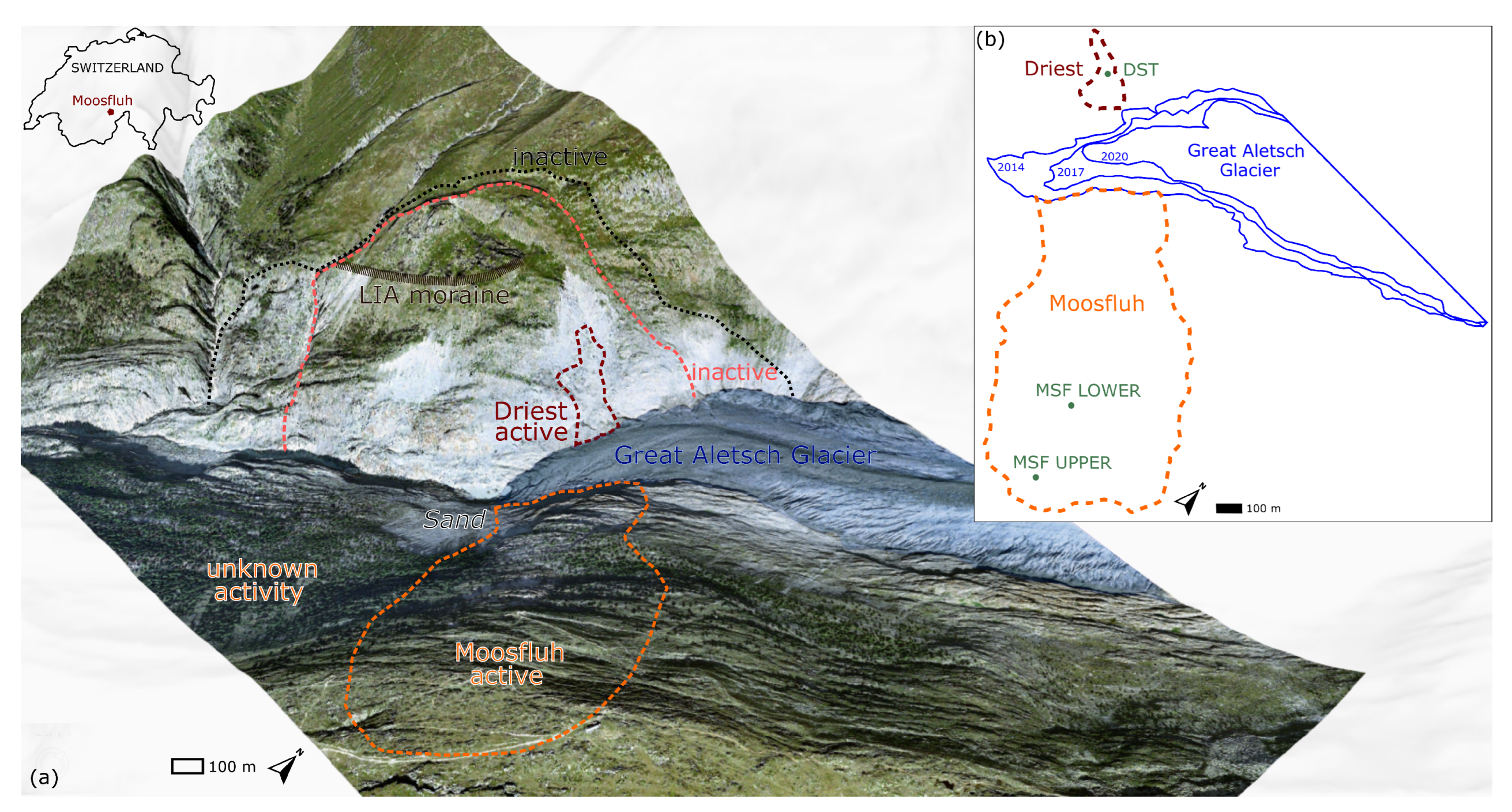
For the performance tests, we selected the landslides Driest (DST) and Moosfluh (MSF) at the tongue of the retreating Great Aletsch Glacier, Valais, Switzerland, as in-depth knowledge of the landslides’ history exists, including their vicinity, and thus coverage, in the remote sensing data (
Figure 1) [
9,
41,
42,
43]. The displacement investigations go back to 1967 for Driest [
42] and 1961 for Moosfluh [
26] from available historical aerial images.
Alongside our main goal, the attempt to provide a first generic approach to reduce time and labour-intensive pre-analysis work, we offer answers to the following research questions: (i) which spatial resolution is required to detect slope displacements, (ii) how does the sensor’s spatial resolution affect the accuracy of the modelled displacement magnitude and rate, and (iii) how are DIC input parameters and DIC performance related.
2. Study Sites
The two landslide sites investigated, Driest and Moosfluh (
Figure 1), are located in the glacier flow direction orographically right and left, respectively, at the valley flanks near the tongue of the Great Aletsch Glacier, external crystalline Aar Massif, Switzerland.
The landslides are responding to the ongoing deglaciation, and thus the retreat of the Great Aletsch Glacier since approximately 1850, having a stress-relief debuttressing effect on its adjacent slopes leading to destabilisation [
9,
42,
45,
46]. However, the landslides do not react in a linear response [
9] and the glacier ice may control landsliding [
29], but glacial debuttressing is not a prerequisite [
47].
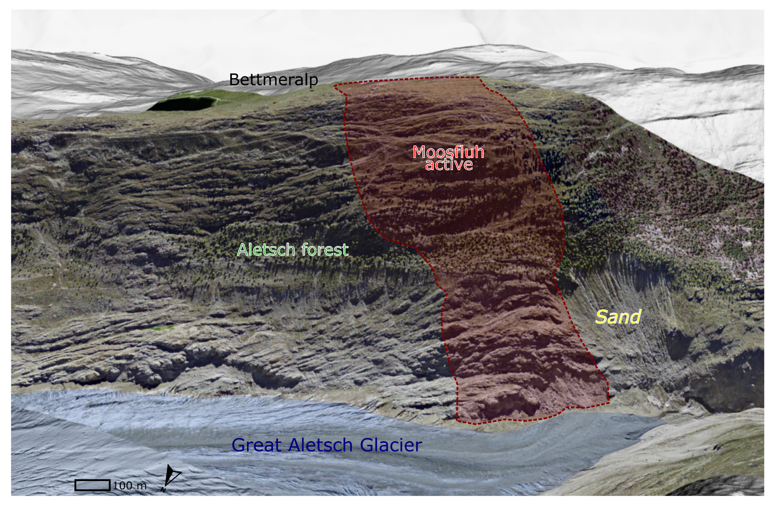
The Moosfluh landslide (
Figure 2) is classified as a deep-seated gravitational slope deformation (DSGSD) [
48] with depths up to 170 m, a volume of 75 Mio. m
covering approximately 1,000,000 to 1,320,000 m
[
26,
44].
Due to its complex evolution and changing behaviour, the history, morphology, and structure were reconstructed, described, and mapped in detail, and the displacement behaviour studied in depth with numerous remote sensing data and techniques. The Moosfluh showed typical velocities of DSGSDs characterised by slow deformation rates of several millimetres per year over long periods (ERS 1/ENVISAT-IS2, 1976–1995 with <50 cm, ∼3 cm a
) with no significant movement measured [
43]. Extensive investigations employing DIC on aerial images (1976, 1995, 2006), GPS measurements (summers 2007, 2008) complemented with InSAR displacement analyses (1992–2008 on ERS 1/2, JERS, Envisat, ALOS, and TerraSAR-X revealed its reactivation in the 1990s (∼5 cm a
in 1992), accelerated beyond typical DSGSD movement rates (>30 cm a
, summer 2008), modified (shift towards the upvalley NE-direction), and decreased thereafter [
43,
49,
50]. Another multi-sensor approach analysed InSAR data (ERS 1/2, JERS, Terra SAR-X, 1992–2012) and LiDAR data (TLS 2012–2015, ALS 2005) confirming previous findings [
9]. In 2015 the erosional feature “Sand” was activated as secondary rockslide (
Figure 1) [
26,
44]. A further re-acceleration of the entire Moosfluh in fall 2016 with three subsets and a total volume of 7 Mio. m
changed the typical DSGSD with a slow, nonhazardous behaviour into a highly active, hazardous mass movement [
26]. This recent acceleration was investigated on the basis of aerial historic images (1961–2016), DIC analyses (orthophotos, 2005–2016) including data from high resolution geodetic monitoring, and webcam time lapse imagery [
26,
44] showing that local slope kinematics were changed from predominantly toppling into a mixed toppling/sliding mode [
26]. Current data analyses combining DInSAR (S-1) and DIC (S-2) (early spring to autumn 2017) [
27] and DIC (UAS, 11–16 July 2018) [
29] show that the landslide is sensitive to heavy rainfall events such as in 1999 and 2005, as well as to the strong glacier retreat (2004–2005), but is currently slow moving (∼30 cm a
) [
26].
On the opposite slope, the Driest rock slope instability is located (
Figure 2). Here, smaller rock slide activities at the end of the 1960s and beginning of the 1970s were documented [
51]. Between 1967 and 1995 a larger continuous rock slide with a total displacement of ≤2 m, including surface subsidence in the upper and uplift in the lower part, were described as a vertical rotation. Its displacement was derived with DIC using CIAS and height changes based on the digitally generated DEMs from stereo photography [
42,
45]. For a longer time range of 30 years (1967–2006), 1.5 to 4.2 m displacement were measured employing DIC (NCC) based on 0.2 m resolution orthoimages [
52]. Surface change calculations using ALS showed significant surface changes for 2005–2011. The main upper sector showed mainly downslope movement (≤0.2 m) including sedimentation and outward movement at the toe region. Higher changes of 20 m were documented for the NE-flank caused by landslide failure [
9]. Once again, all studies conclude that the trigger of this instability is attributed to the retreat of the Great Aletsch Glacier, and argue that this activity is pronounced for the period since the 1990s [
9,
45,
52].
3. Materials and Methods
In order to generate DIC formulas to determine the most suitable spatial resolution for certain displacements and to estimate the most efficient correlation window size, we selected various remote sensing sensors usually employed for these purposes. It is impossible to consider the numerous algorithms available. Hence, we first keep the algorithm constant, focusing on one, which gives the most freedom in defining the window sizes and includes a pre-processing of image co-registration. Second, we endorse the principles of open code and open data, and therefore selected a free algorithm and freely available data. However, it should be noted that the MATLAB software required to run the code is not open-source.
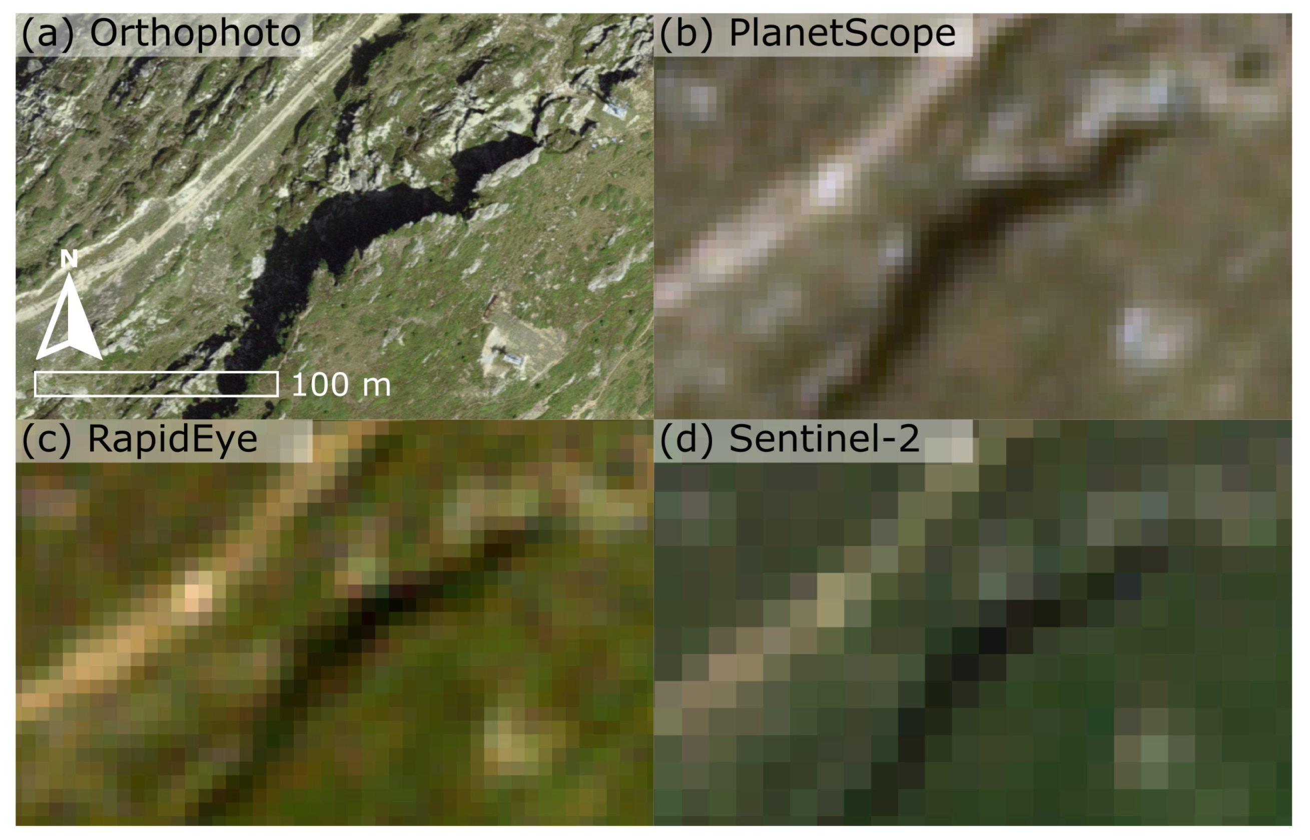
The data set consists of high resolution aerial orthophotos and medium- to high- resolution multispectral satellite images (
Table 1). Our intention was to use both freely available optical data and code. The swisstopo orthophotos (0.1 m) were provided courtesy of ETHZ library (
Table 1 and
Table 2) and defined the temporal constraints. We selected several of the most suitable satellite images in terms of image quality and time proximity to the aerial acquisitions for the DIC displacement calculations (
Table 1,
Figure 3).
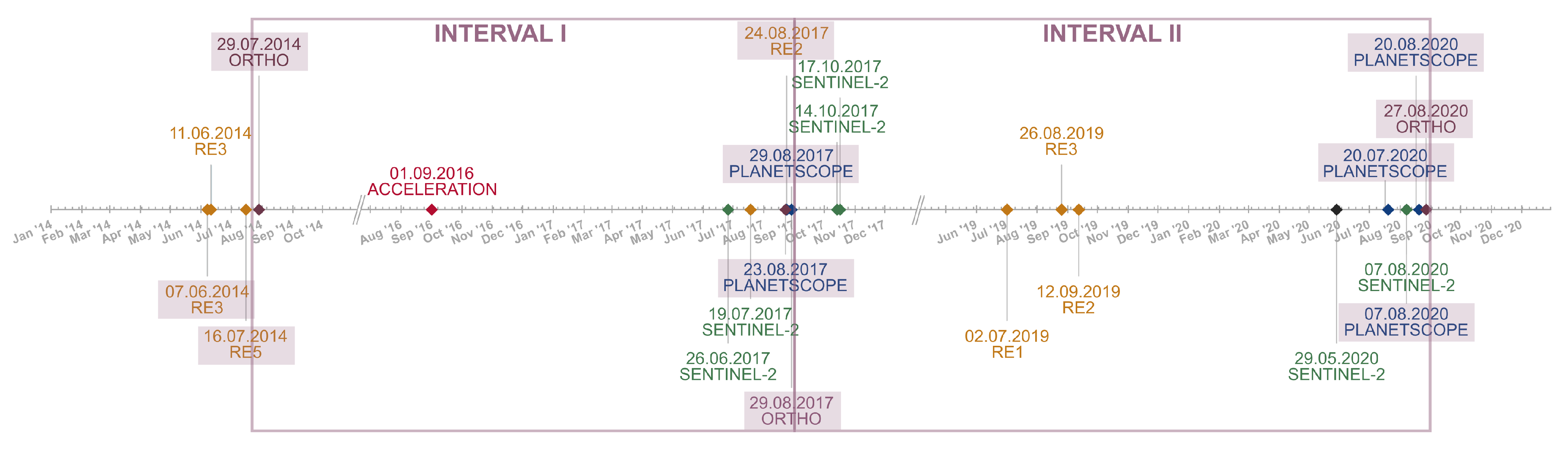
The aerial images (27 September 2014, 29 August 2017, 27 August 2020) defined two investigation intervals, 2014–2017 (I) and 2017–2020 (II), and, thus, our corresponding satellite image pairs (
Figure 3,
Figure 4 and
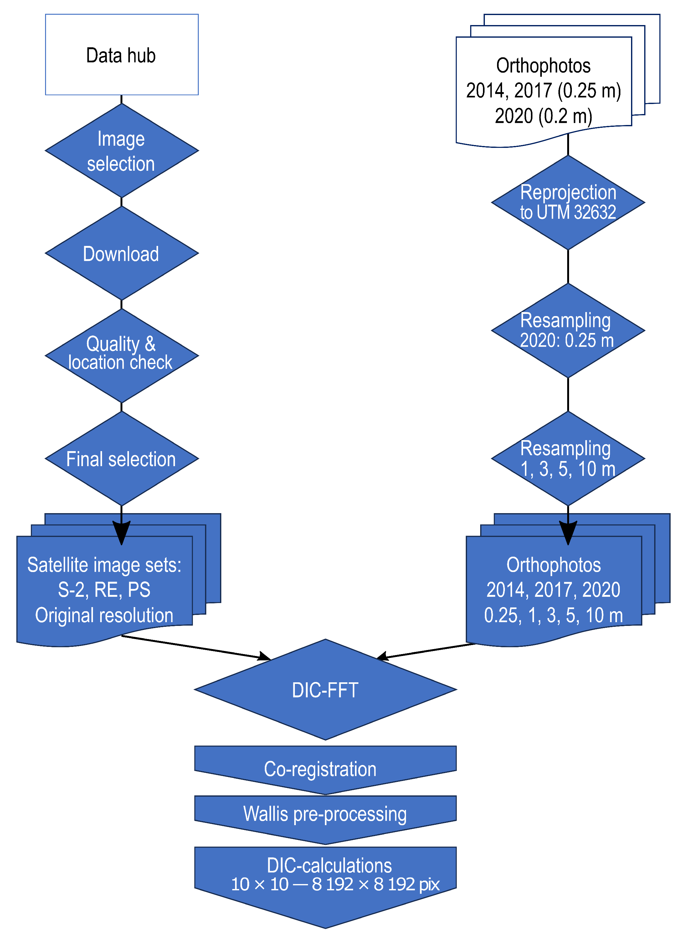
Figure A4). Images were reprojected from CH1903+/LV95 to UTM 32632 and merged to cover the relevant study site (
Figure 5). For consistency, we resampled the orthophoto data sets at a common resolution of 0.25 m (see
Table 1) as the original resolutions varied (see
Table 2, personal correspondence swisstopo).
As RapidEye satellites reached their end of life in March 2020, their snow-free images were available until autumn 2019, and thus covered interval I. In contrast, PlanetScope images for our study site have been available since June 2017, hence cover interval II (
Table 1).
Multispectral S-2 images from the European Copernicus Program have been available since February 2015, thus providing additional data for interval II. From the Copernicus SciHub (
https://scihub.copernicus.eu, accessed on 15–31 July 2022), we downloaded S-2 (image pairs of the same orbit R065, R108, tile T32TMS) and RapidEye imagery, while PlanetScope images were downloaded from the Planet Explorer data hub (
https://account.planet.com, accessed on 17–31 July 2022). We focused on images temporally close to the aerial acquisition dates (see
Figure 3 and undisturbed by meteorological constraints (e.g., clouds, cloud shadow, snow cover)), image errors (false colours, interband co-registration, over-saturation, blur); all were reflectance-corrected images (bottom-of-atmosphere). After the download, we refined our selection following a visual quality and positional check in QGIS (
Figure 5). For PlanetScope images, we focused in particular on interband co-registration errors, false colours, and co-registration errors, as PlanetScope images are often affected by these quality issues [
53].
RapidEye images for our study site were rather limited, especially after elimination of cloud-affected and snow-covered scenes, which left us with two image pair constellations, 7 June 2014–24 August 2017 and 16 July 2014–24 August 2017 (
Figure 3). The intervals cover ∼1174 days and ∼1135 days, respectively (
Table 1). Apart from natural meteorological constraints, selecting suitable PlanetScope Tiles enabled us to disregard many available scenes due to a lack of quality, such as misaligned or blurry images, inter-band co-registration and colour errors. This substantially reduced our data set. We selected two (23 August 2017, 29 August 2017) PlanetScope tiles as reference images and three (20 July 2020, 7 August 2020, 20 August 2020) as secondary images, which resulted in six combinations for the DIC calculations, as these were the only qualitative options (
Figure 3). Although the revisit rate of S-2 is five days and doubled to ten days if the same orbit tracks are considered, the results for comparative analyses such as change detection and DIC are enhanced if image pairs are of the same orbit [
13]. Apart from natural meteorological constraints, six scenes were chosen as suitable. However, due to our requirement that scenes come from the same orbit to reduce co-registration errors [
13], four DIC combinations remained: one DIC pair for R065 and three for orbit R108 (see
Table 1,
Figure 3).
For further analysis and as a data base for our formulas, we resampled the orthophotos (0.25 m) at 1 m, 3 m, 5 m and 10 m resolution to be similar to the original resolutions employing the cubic convolution method using GDAL of RapidEye, PlanetScope, and S-2 (
Figure 5). This first allowed us to compare the DIC performance of both the original input data sets (e.g., orthophoto 0.25 m vs. RapidEye 5 m) and of the input data sets of the resampled orthophotos to the original image at the corresponding resolution (e.g., orthophoto 5 m vs. RapidEye 5 m). Secondly, it enabled us to calculate our formulas.
We calculated displacements using the open-source area-based DIC-FFT, which is based on the Fast Fourier Transform and runs on MATLAB (available on GitHub
https://github.com/bickelmps/DIC_FFT_ETH, accessed on 30 June 2022) [
23], and we visualised, analysed and compared the data and results in QGIS. In DIC-FFT we first co-registered the images on sub-pixel accuracy to reduce image shifts and maximise the matching of the true pixel-offset to approximate the real ground motion. Secondly, each DIC iteration was calculated with window sizes ranging from 10 × 10 to 8192 × 8192 pixels (
Figure 5). Thus, we went beyond the sizes of 64 × 64 and 128 × 128 pixels, recommended by other studies, to obtain a good balance between correlation and accuracy [
32,
54].
Pre-processing, utilising Wallis filtering (the code’s intrinsic dynamic contrast enhancement routine), enhanced image quality in well-lit or poorly lit areas, resulting in improved DIC results for the orthophotos and some of the RapidEye and PlanetScope image pairs (
Figure 5). Employing an oversampling factor of four, which generally increases processing time [
23], also somehow improved the DIC results for S-2, PlanetScope and RapidEye images, with negligible effects on the orthophotos. The S-2 DIC calculation band B08 SWIR (shortwave infrared band, 842 nm wavelength) returned clearer results than the available TCI product (true colour image, a composite of B02 (blue), B03 (green) and B04 (red)). We did not apply any post-processing filters, and thus kept the results raw. Based on active landslide areas and estimated displacements from earlier studies [
26,
27,
29,
42], we selected matching DIC results from the different image pair combinations (
Table 1).
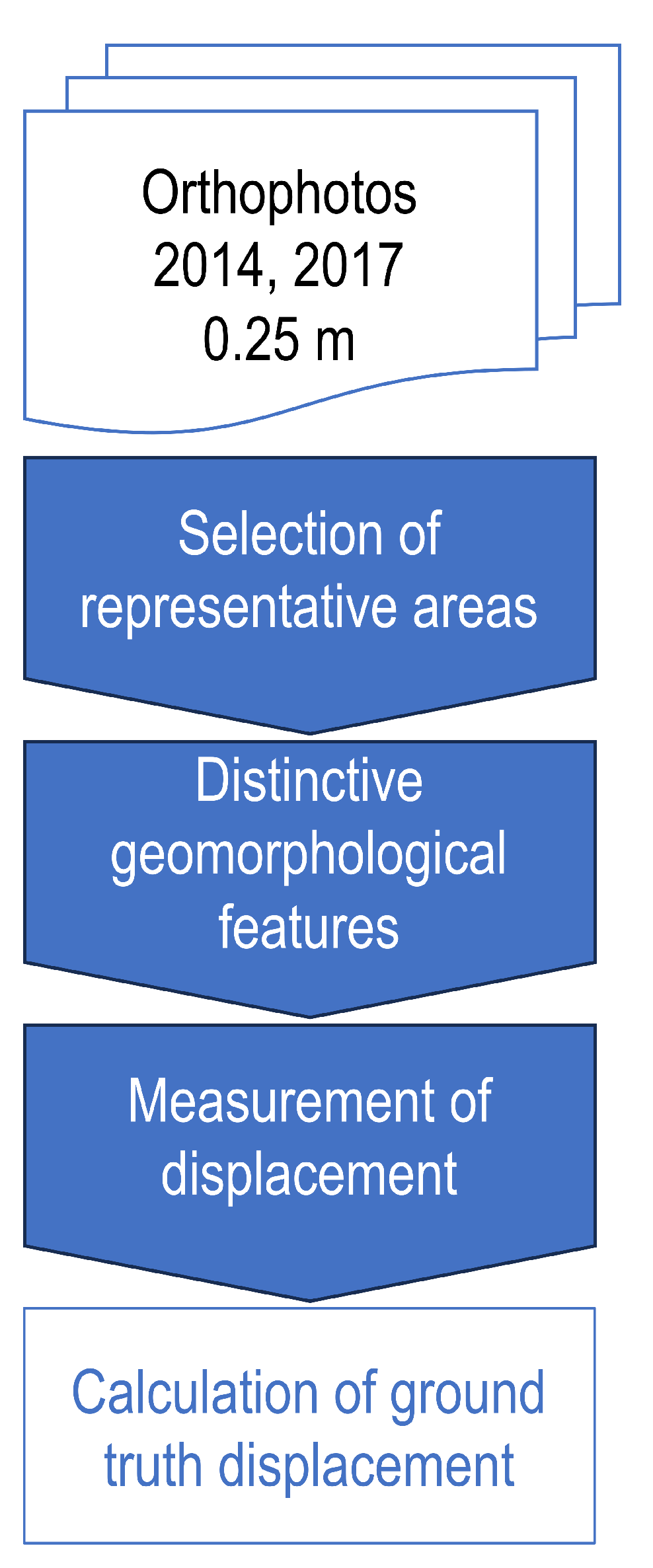
Next, to validate and assess DIC results, thus to estimate measurement uncertainties [
55] and second, to achieve our main goal to generate formulas, we selected three appropriate areas (see
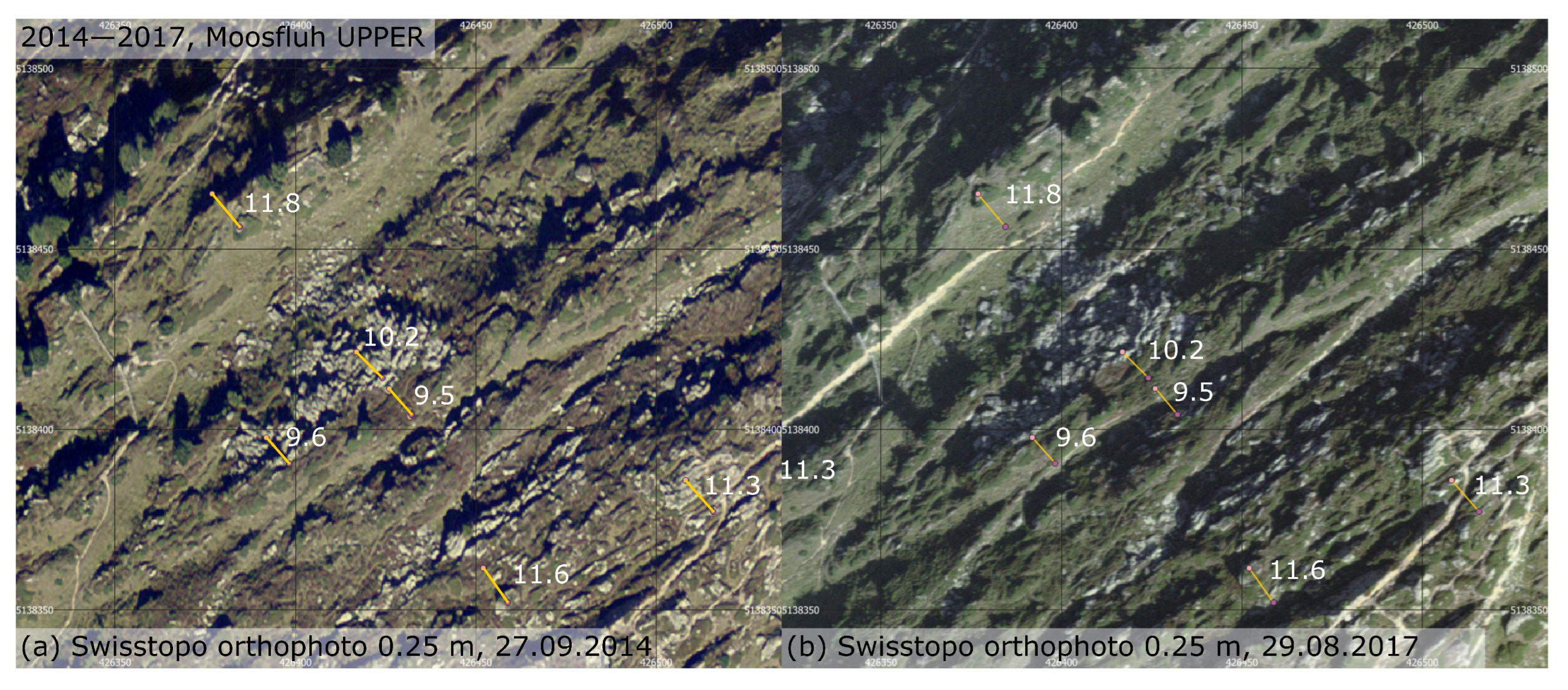
Figure 1). Two areas, a slower (MSF UPPER) and a faster one (MSF LOWER), are in the upslope area of the Moosfluh landslide; the other area is located at the opposite slope on the eastern upvalley area of the Driest landslide (DST). For each of these three representative areas, we selected five to six distinctive geomorphological features (e.g., boulder blocks, paths), identifiable in all orthophotos intervals (I, II), and manually measured their displacements based on the feature’s centre to define our ground truth (
Figure 6 and
Figure 7). The high resolution and accuracy orthophotos served as a benchmark to compare the entire DIC displacement results.
From interval I, we collected the modelled DIC displacements for each measurement point: for (i) each data set, i.e., orthophotos at 0.25 m, 1 m, 3 m, 5 m, and RapidEye at 5 m as well as (ii) the entire range of different window size calculations (10 × 10 to 8192 × 8192 pixels) (see
Figure 5). For the pre-defined areas, we measured the DIC displacement results on the basis of (i) the original resolution of the RapidEye tiles and the orthophotos at four different spatial resolutions, as well as of (ii) the DIC orthophoto results at differing window size parameters. In so doing, the average displacement of the surrounding manual measurements was calculated and subtracted from each single point measurement for both the calculated DIC displacements at (i) different resolutions and (ii) window sizes.
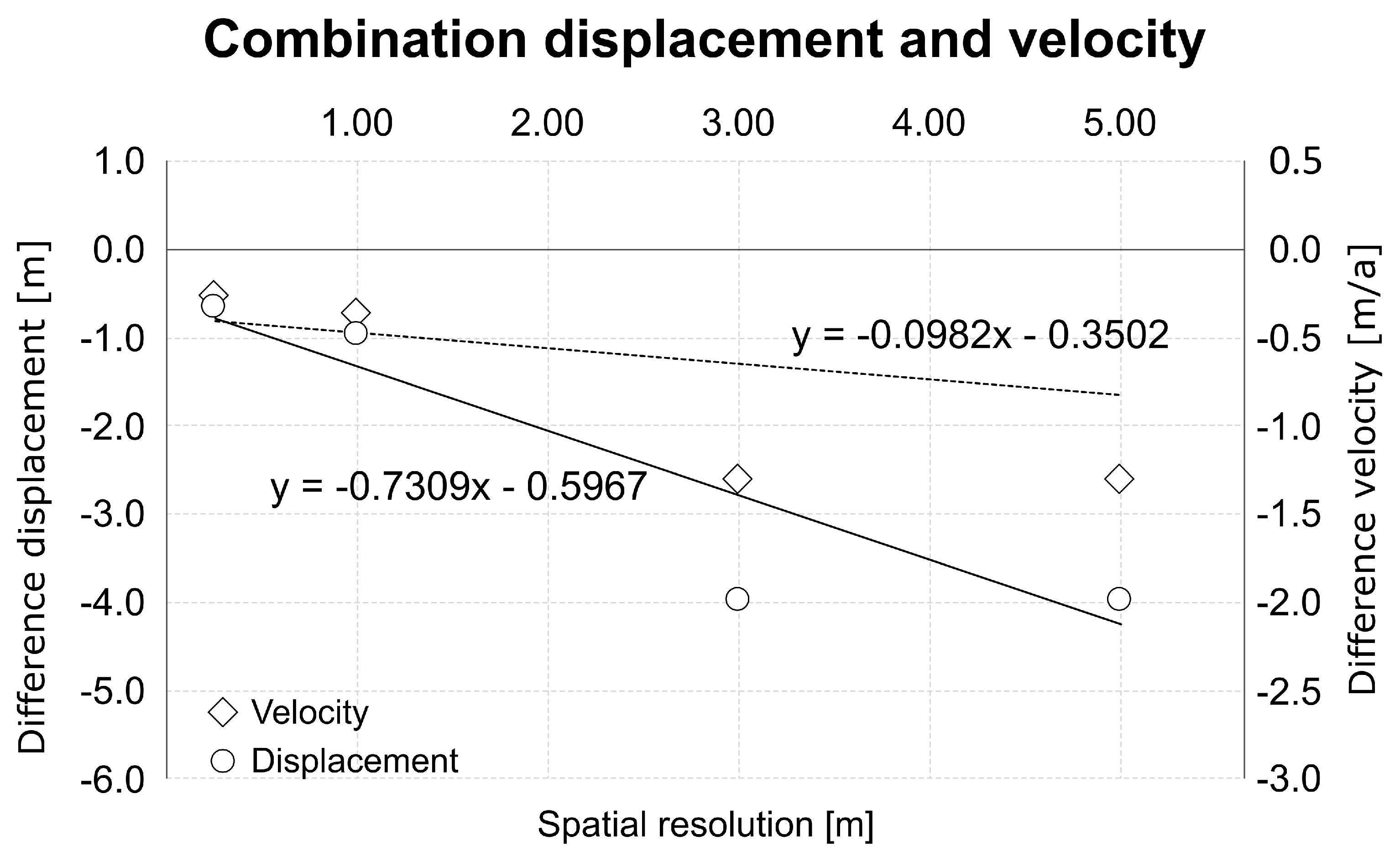
For (i), the DIC performance was calculated for total displacements and averaged velocity values (displacement per year). These measurements permitted us to estimate the relation between the DIC calculations and the benchmark, thus the measurement accuracy of the modelled DIC results. Finally, the resulting differences were plotted against the spatial resolution for both the total displacement and the velocity per year. Accordingly, we derived our first formula describing the DIC performance in relation to the spatial resolution of the input data.
For (ii), in order to estimate the influence of the window size on the DIC results, derived from the orthophotos at 0.25 m for the three measurement points (DST, MSF UPPER, MSF LOWER), we calculated their mean velocity per year. Thereafter, to derive the second formula we plotted the difference in velocity against the window size ranges.
And finally, for (iii), we show exemplarily how the formulas are employable to displacement data estimating the potential offset if a coarser spatial resolution or window size are taken. Therefore, took the formulas and employed them on displacement calculations from this study showing a displacement curve with four observations, thus three intervals. The data represents debris flow landslide in the Sattelkar, Austria, from 24 September 2019 to 11 September 2020 reflecting an acceleration. We calculated the formulas to show the differences regarding various spatial resolutions (1 m, 3 m, 5 m) and window sizes (32 and 64 pixels) based on displacement measurements from the Sattelkar study [
34].
4. Results
This section outlines the results of the studies calculating the total displacement for the orthophotos at several resolutions (interval I and II), RapidEye (I), PlanetScope (II), and S-2 (II) as a basis to define a generic approach identifying the most suitable spatial resolution and window size parameters. Therefore, we present the results from estimated displacement and velocity differences and compare them to (i) the image input resolution and (ii) the various window sizes for the orthophotos at 0.25 m resolution.
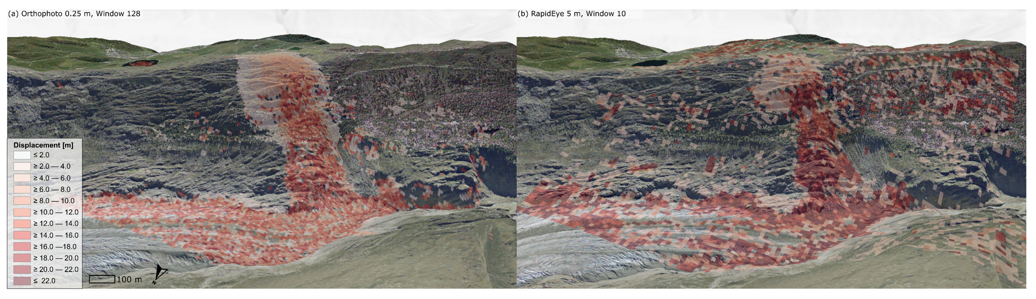
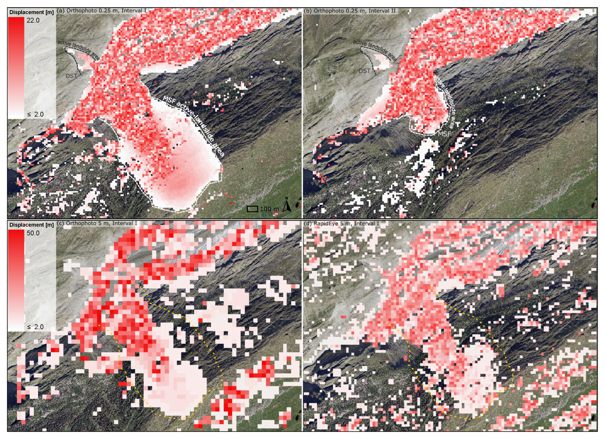
Figure 8 presents the results from the DIC calculations for interval I (2014–2017) for (a) the orthophotos at 0.25 m, (c) the orthophotos resampled to 5 m, and (d) the RapidEye scenes at 5 m, as well as for (b) interval II (2017–2020) the orthophotos at 0.25 m. For interval I, the active area of the Driest is ∼25,249 m
and the Moosfluh is ∼740,000 m
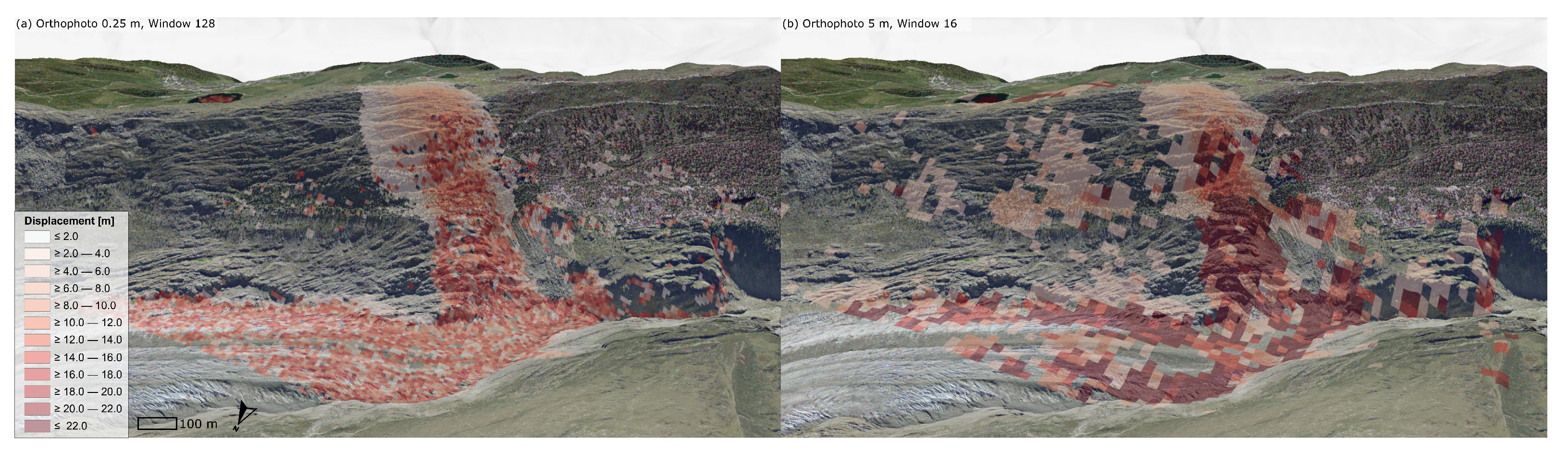
when displacements below 2 m are excluded. Homogeneous areas for the landslide areas DST, MSF UPPER and MSF LOWER are discernible while the glacier and the lower MFS “Sand” area return ambiguous signals. For a direct comparison of DIC results in a 3D perspective for orthophoto pairs (0.25 m (a) and 5 m (b)), interval I, see
Figure 9.
Results for interval I for the orthophoto pair (27 September 2014–29 August 2017, 0.25 m) show unambiguous areas for Moosfluh upper landslide body including the edge area around the landslide’s main body with total displacement values between 2 to 10 m as well as an active area of Driest with 6 to 9 m (
Figure 8a). This is similarly reflected in the RapidEye results at the original 5 m resolution (16 July 2014–24 August 2017), however with a less clear displacement for the Driest area (
Figure 8d).
For interval II, the orthophoto pair (29 August 2017–27 August 2020, 0.25 m) (
Figure 8b) returns coherent signals for the Driest landslide only. For the upper part of the Moosfluh landslide body, there is no coherent signal in any of the data sets (orthophoto, PlanetScope, S-2), hence comparisons are not possible (cf.
Appendix A Figure A1). The PlanetScope pair (23 August 2017–20 August 2020) clearly demarcates areas with no signal in both MSF LOWER and MSF UPPER, while the lower “Sand” zone of MSF and the glacier are recognisable due to ambiguous signals (
Appendix A Figure A1a). Therefore, we dismissed this period from our study and excluded it from the formula generation.
For the following analyses to generate our formulas, we only considered areas of unequivocal signals. Manually measured from the orthophotos (
Figure A4), the displacements average 10.66 m, 5.47 m and 8 m for MSF LOWER, MSF UPPER and DST, respectively. Compared to the DIC results (window sizes 64 × 64 and 128 × 128), the differences for MSF UPPER are 0.53 m, −0.47 m, −1.47 m, −2.97 m (orthophotos at 0.25 m, 1 m, 3 m, 5 m) and −0.47 m on average (RapidEye at 5 m); for MSF LOWER −1.16 m, −1.66 m, −2.66 m, −4.66 m (orthophotos at 0.25 m, 1 m, 3 m, 5 m) and 0.47 m on average (RapidEye at 5 m); and for DST 0.22 m, 0.28 m, −7.27 m, 7.27 m (orthophotos at 0.25 m, 1 m, 3 m, 5 m) and −7.27 m on average (RapidEye at 5 m).
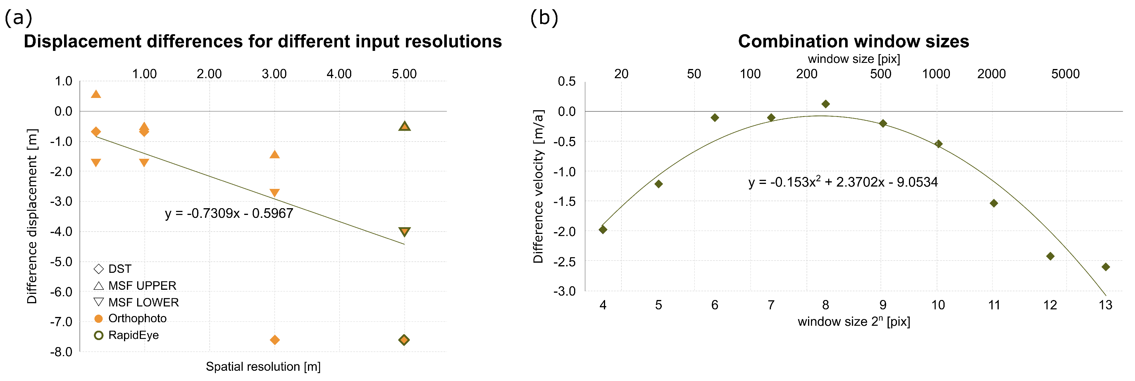
On the basis of the orthophotos (0.25 m), the resampled orthophotos (1 m, 3 m and 5 m) and the RapidEye images (5 m), for MSF LOWER, MSF UPPER and DST, we observed a linear relationship between the image spatial resolution and the DIC performance of displacement (m) in terms of estimated differences versus the resulting error:
The combination of the three measurement points indicates a decrease for both the difference in total displacement (
Figure 10a) and velocity (
Appendix A Figure A3). Thus, for our case studies a displacement of at least 1 to 2 pixels is required to yield distinguishable signals, to be detected as a mass movement employing DIC. We can support this as we observe with a higher spatial resolution a lower deviation between the DIC-modelled and the real displacement (Equation (
1)).
The range of different window size DIC calculations using the 0.25 m orthophotos for all measurement points enabled us to determine a relation between the size of the correlation window (16 to 8192 pixels) and DIC performance (difference/error). As the window size is typically a power of two, the graph is plotted with both the window size in pixels as well as the power of the window size, n, against the velocity (m a
). Note that the relationship between the window size and window size power is a power relationship:
Once the log
value of the
window size,
n, is taken, the data may be correlated with performance with a quadratic equation, with R
= 0.9691:
Rather than directly comparing the window size with velocity difference, first the log of all window sizes with recommended base 2 must be taken. The fit is then with
x for window size and y for difference in velocity:
For the orthophoto resolution of 0.25 m, the window sizes of 16 and 32 pixels reflect a difference from the averaged velocity between −2 m a
and −1.2 m a
. We observe with an increase in window size, a decrease in the velocity differences, ranging around zero for 64, 128, 256 pixels with values of −0.09, −0.09, and 0.13 m a
, respectively. However, with further increasing window sizes, the difference also increases with a cut off at window sizes beginning at ∼512 pixels with a difference of −0.2 m a
and noticeably for windows greater than 1024 pixels showing a difference of −0.54 m a
and for 2048 pixels a difference of −1.54 m a
(see
Figure 10b).
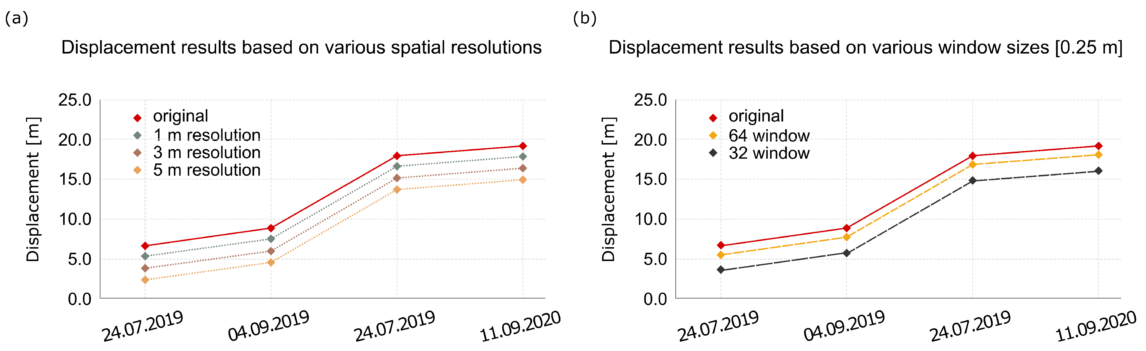
Our formulas were applied for different spatial resolutions (1 m, 3 m, 5 m) and window sizes (32 and 64 pixels) to the time series displacement values of the Sattelkar study site [
34]. They are visualised in
Figure 11 and reflect our observations from the formulation graphs (see
Figure 10). Both variables, the spatial resolution and the window size, show significant differences with reduced displacements. In general, with a lower spatial resolution, the estimated displacement difference increases up to 4.25 m for the difference between the original displacement and the calculated displacement for 5 m. Similarly, the calculated values approach the original displacement values. For a window size of 32 pixels, it differs by 3.09 m and approaches a similar value as the original with a difference of approximately 1 m for 64 pixels.
5. Discussion
The goal of this study was to suggest a first generic approach and therefore to reduce the time and labour intensive manual optimisation work. In order to achieve this goal, determining (i) the minimum required spatial resolution, (ii) how the spatial resolution affects the DIC accuracy provide the basis for the first part of our generic approach, and (iii) how DIC parameters and performance are related provide the basis for the second part.
For interval I, the upper area of the Moosfluh landslide and the Driest reflect homogeneous, unambiguous displacements from successful correlations (
Figure 8a,c,d). For I, past studies report that after the acceleration in 2016, there were some further discernible ground motions in 2017 [
27,
29] with enhanced velocities beyond a classic DSGSD (11 to 22 m between 26 June 2017–17 October 2017) [
26,
27]. For II, however, it appears that the entire landslide became inactive as areas MSF LOWER and MSF UPPER did not reflect any displacement signal. Nevertheless, the lower zone is visible in intervals I and II, reflecting decorrelation due considerable surface alterations and displacements exceeding the matching capability of the DIC. For that reason, the generic formulas were calculated using results from interval I.
Focusing on the spatial resolution, (i) and (ii) are discussed. Comparing the DIC performance for the orthophotos from 0.25 m to 5 m spatial resolution and RapidEye (5 m), we observe a relation between the image spatial resolution and the DIC-performance, i.e., the difference between manually measured displacements (see Equation (
1),
Figure 10a). Thus, the higher the spatial resolution, the better the DIC performance. While DIC results from high resolutions (0.25 m, 1 m) ranging between 0.53 and −1.66 m are in good agreement for MFS UPPER, MFS LOWER and DST, they have slightly different displacement magnitudes. At a resolution of 3 m only the slower MFS UPPER performs better with a low difference (−1.47 m) whereas MFS LOWER (−2.66 m) and DST (−7.72 m) in particular have increased differences between manually measured versus DIC results.
The modelled results from RapidEye at the original 5 m spatial resolution and orthophotos resampled to the same resolution correspond to a high degree in both the DIC displacement maps (
Figure 8c,d) and the values for MSF UPPER, MSF LOWER and DST (see
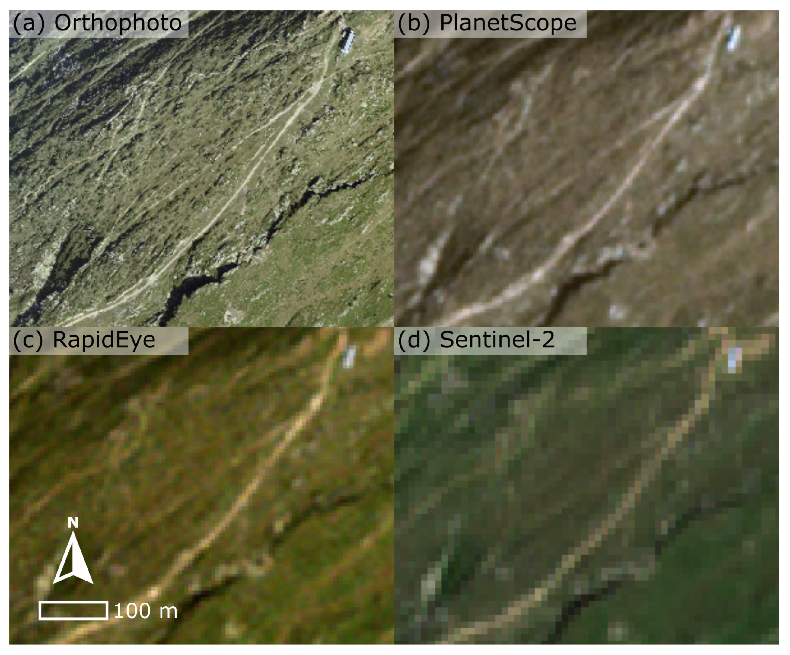
Figure 10a). These similar DIC results and calculation differences allow us to conclude that the downsampling to this level does not negatively influence the result as it matches a sensor at the same resolution. The downsampling generalises, thus homogenises features e.g., a bush, which is clearly recognisable in a 0.25 m resolution RGB imagery, while it vanishes at a spatial resolution of 5 m (see
Figure 4 and
Figure A4). However, this loss of heterogeneity which reduces noise at a lower resolution could affect the result using a higher spatial resolution for the DIC input. For instance, differences in vegetation or visible cast shadows, which are detectable using DIC, can impact the results. This may lead to an incorrect deformation signal.
Based on our direct manual measurements compared to the DIC results for a range of spatial input resolutions for displacements from DST and MSF (i) and (ii), we assume that at least a displacement magnitude of 1 to 2 pixels is required to be detected as a mass movement using DIC. From this follows that for these landslide sites a sub-pixel detection is questionable and not realistic, and second, a sensor with at least 5 m resolution is required to capture this displacement (
Figure 8), as supported by our suggested Equation (
1) (see
Figure 10a).
DIC results for the orthophoto in interval II reflect correlated displacements for DST as well as slope wasting processes at the foot of the inactive DST (
Figure 8b). In accordance to our suggested Equation (
1), a landslide with characteristics similar to the MSF in terms of displacement magnitude and size, we assume that a spatial resolution of 5 m and higher is sufficient to identify and measure displacements (
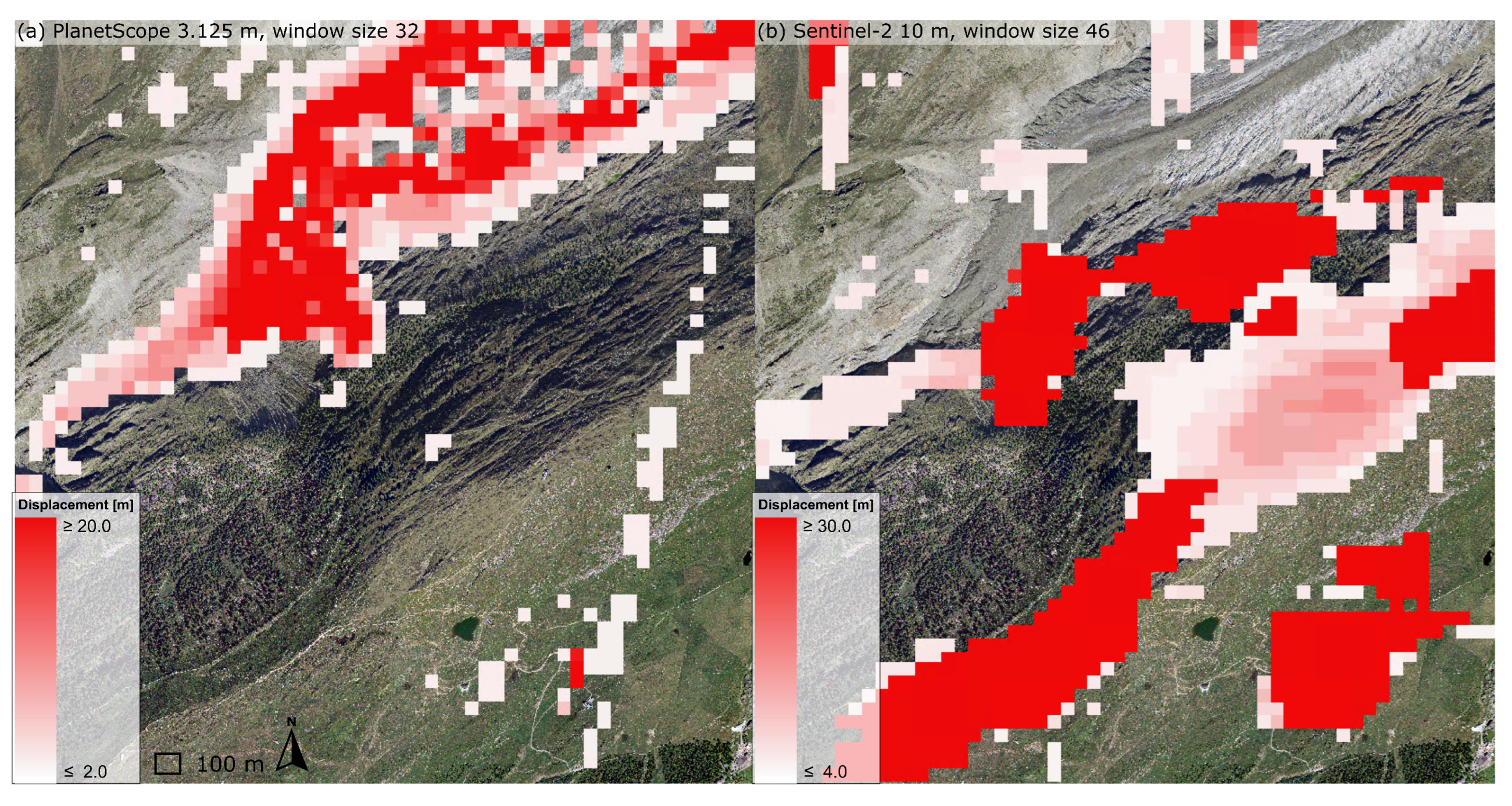
Figure 8c,d). In contrast, as observed in our results for DIC on S-2 (10 m), a sensor of medium resolution failed to correctly identify a displacement (
Figure A1b). For a clear signal, 2 pixels would require 20 m displacement for an investigation interval. We manually measured 10.66 m in the faster MSF LOWER, and the DIC results for input resolutions of 0.25 and 1 m averaged displacements of 9.5 m and 9 m, respectively (window sizes 64 × 64 and 128 × 128). A case study for the large Harmalière landslide, France, with ∼1,800,000 m
successfully detected displacements using S-2 scenes and COSI-Corr for DIC calculations [
13]. Comparing the considerable difference in landslide sizes, we assume that the Driest (∼25,249 m
) and Moosfluh (∼740,000 m
), are too small with regard to their total displacement and size to be investigated using a senor of 10 m spatial resolution like S-2 and beyond, such as Landsat 8 (30 m). This is in accordance with the advice from the Harmalière study that small landslides are undetectable with medium resolution satellites such as S-2 [
13]. Consequently, our results (Equation (
1)) confirm that this resolution does not meet the criteria to detect the displacement which occurred between 2014 and 2017 for the corresponding motion areas of Driest and Moosfluh. Thus, a higher resolution than S-2 is required. With regard to (iii), the relationship between DIC parameters and performance reveals a notable effect when using different window sizes during correlation. Larger window sizes capture substantial displacements but reduce spatial resolution. Conversely, smaller correlation windows may fail to capture large displacements, resulting in ambiguous signals caused by decorrelation and mismatches. To achieve better correlation, especially when the surface undergoes minimal change, our proposed generic approach, Equation (
3), assists users in pre-defining an optimal window size range. We observe an increase in performance with larger DIC window sizes, indicating that larger window sizes lead to more accurate modelled displacements (
Figure 11). However, beyond a certain threshold, further increases in window sizes lead to decreased accuracy (
Figure 10b). For window sizes of 64, 128, and 256 pixels, the accuracy is highest, hovering around zero (m a
). However, with window sizes beyond 512 pixels, the performance deteriorates. While our formula considers very large window sizes to explore and validate this effect, these results are inherently noisy. Thus, the formula is recommended for a range of window sizes below the cut-off value (
Figure 10b). Although the error does not significantly increase, i.e., the performance only drastically deteriorates for values above
, the model is recommended for values
. For our case studies, the most suitable window sizes are 64, 128, and 256 pixels, reflecting the optimal trade-off between velocity difference and error (
Figure 10b). A window of 256 pixels slightly overestimates the true displacement by −0.2 m, confirming general statements about window sizes and precision versus accuracy [
7,
35]. The larger the DIC window, the higher the resulting signal-to-noise ratio and precision of displacement estimates. More pixels enhance matching, but accuracy declines due to the averaging effect of the increased window size. Thus, a larger window includes more pixels for a larger search area, resulting in smaller potential mismatches. Our findings indicate a range of optimal ratios between accuracy and precision (
Figure 10). With the generic Formula (
3), we provide an initial approach for users to approximate this range without the need for time- and labour-intensive trial and error calculations [
56]. This is illustrated using displacement values from a different study, demonstrating the ability to estimate the most suitable window size parameters and the necessary spatial resolution for input images. In line with previous findings on spatial resolution versus performance, our study further emphasises that the most suitable image resolution falls around 0.25 m, aligning with the common resolution for classical aerial image acquisition campaigns using aeroplanes and modern UAS, providing optimal performance.


