Abstract
Naïve Bayes classification is widely used for landslide susceptibility analysis, especially in the form of weights-of-evidence. However, when significant conditional dependence is present, the probabilities derived from weights-of-evidence are biased, resulting in an overestimation of landslide susceptibility. As a solution, this study presents a semi-naïve Bayesian method for landslide susceptibility mapping by combining logistic regression with weights-of-evidence. The utility of the method is tested by application to a case study in the Kulekhani River Basin in Central Nepal. The results show that the naïve Bayes approach with weights-of-evidence overpredicts the posterior probability of landslide occurrence by a factor of about two, while the semi-naïve Bayes approach, which uses logistic regression with weights-of-evidence, is unbiased and has more discriminatory power for landslide susceptibility mapping. In addition, the semi-naïve Bayes approach can statistically distinguish the main factors that promote landslides and allows us to estimate the model uncertainty by calculating the standard error of the predictions.
1. Introduction
Naïve Bayes has been widely used as a simple but often effective classification system in many disciplines since the advent of computational power. Naïve Bayes refers to Bayes’ theorem about determining the probability (likelihood) of an outcome under certain conditions that are believed to be mutually independent. Recent applications of Naïve Bayes and its variations are reviewed by Wickramasinghe and Kalutarage [1]. In real-world applications, data can be inter-related, violating the independent assumption. Improvements called semi- or weighted-naïve Bayes have been proposed to address this problem. Discussions have been presented on the semi-naïve Bayes classification used to alleviate the conditional independence assumption, for example, Zaida et al. [2].
Landslide susceptibility is defined as the probability of slope failure given a set of geo-environmental conditions [3]. Landslide susceptibility mapping assumes that landslides occur due to similar geological, geomorphic, and hydrological conditions leading to past and present events. Intrinsic variables influencing landslides include geo-environmental factors such as geology, topography, soil type, land use, and drainage pattern, while extrinsic variables include rainfall, earthquakes, and volcanic activities [4,5,6]. Intrinsic variables are usually static, while extrinsic variables are temporal, which is more complex to deal with in practice.
Various approaches have been developed for the evaluation of landslide susceptibility, including heuristic, deterministic, and statistical classification methods [7]. Prominent features of the statistical approach are its high efficiency, low cost, and better and more accurate understanding of the relationships between spatial factors used to identify landslide-prone areas [8,9]. Lee [10] presented a comprehensive review of landslide susceptibility studies, comprising 776 papers published over a twenty-year period (1999–2018). The most common were statistical methods, such as logistic regression (14% of the total number of articles) and frequency ratio (13%), with weights-of-evidence (6%) ranked seventh. Reichenbach et al. [11] presented a critical review of statistical models of landslide susceptibility, covering 565 peer-reviewed articles from 1983 to 2016, and reported that the more common statistical classification methods for landslide susceptibility assessment are logistic regression, neural network analysis, index-based, and weights-of-evidence. No single method proves to be superior to all others under all circumstances. Therefore, it is argued to combine multiple methods to obtain an “optimal” model, which could outperform individual models [11,12].
Weights-of-evidence is a naïve Bayesian classification popularized by Bonham-Carter et al. [13,14] for analyses of the occurrence of mineral deposits. Zhan and Agterberg [15] provide an overview of weights-of-evidence modeling in the field of mineral exploration. Weights-of-evidence has also become very popular in assessing landslide susceptibility as it allows a straightforward interpretation of the relationship between landslide occurrence and causative factors. Early examples are Lee et al. [9] and Van Westen et al. [16]; more recent examples worth mentioning are [17,18,19,20,21,22,23]. However, none of these studies use weights-of-evidence to estimate the likelihood of a landslide. Instead, a technique proposed by Bonham-Carter [14] is used to compare the weights obtained for the presence or absence of causative factors and use the contrast of these weights to map landslide susceptibility. In addition, in all applications, the conditional independent assumption is rarely verified, nor are its consequences considered, and theoretical or technical improvements are rarely explored.
In the field of mineral exploration, violations of conditional independence between factors have received more attention, e.g., [15,24,25], and it is recognized that, when there is significant conditional dependence, probabilities derived with weights-of-evidence are biased upwards and result in over-estimation [25]. In the absence of bias, the mean of the posterior probabilities should be equal to the prior probability for all observed events used to train the model, which can be tested for statistical significance [14,24]. For example, Bonham-Carter [14] argued that the difference should not exceed 15%.
Improvements for weights-of-evidence have been proposed in the field of mineral exploration [15]. Improvements are mostly based on combining weights-of-evidence with logistic regression, as the two methods belong to the family of loglinear models and yield similar results when the conditional independence assumption is satisfied [15,25,26,27]. Unlike weights-of-evidence, logistic regression does not have to satisfy the assumption of conditional independence and thus has a wider range of applicability, although it is computationally intensive.
The aim of this study is to present an unbiased, semi-naïve Bayesian classification method for mapping landslide susceptibility by combining weight-of-evidence and logistic regression. The value and feasibility of the method are tested and illustrated by application to a case study in the Kulekhani River Basin in Nepal.
2. Materials and Methods
2.1. Methods
Following the work of Bonham-Carter [14], the conditional probability of landslide given a set of causative factors can be expressed using Bayes’ theorem as
where means a landslide, is a set of factor classes where i denotes the factor and j the factor class, is the posterior conditional probability of a landslide when is present, is the prior unconditioned probability of a landslide, is the probability of when is present, and is the unconditioned probability of .
Assuming the factors are independent, the probabilities and can be calculated by using the chain rule
where n is the number of factors. Similarly, the conditional probability of no landslide can be expressed as
where means no landslide, and is the posterior conditional probability no landslide occurs when is present; obviously . Combining Equations (2) and (3) gives
The probability of a landslide is now expressed in the form of odds [14]. Since multiplications and divisions of probabilities can be cumbersome, it is better to use a log transformation
Since the log of odds is the logit function, , this can also be written as
where are factor class weights given by
The predictive strength of each factor class can be evaluated with the information value IV, defined as [28]
and the total predictive strength of each parameter can be obtained by summation over all classes of a parameter
The IVs can be divided into different ranges that allow interpretation of the predictive power as shown in Table 1 [28] (p. 81).

Table 1.
Evaluation criteria for the predictive power of information values [28].
Equations (6) and (7) allow estimating the conditional probability for landslides based on a training set of observed landslides and causative factors, whereby the probabilities , and are derived from the areas and overlaps of landslides and factor classes. However, the outcome may be biased because it is not guaranteed that all factors are independent with regard to landslide occurrences. This is why it is called a “naïve” Bayesian classification. In practice, conditional independence is never fully satisfied, and posterior probabilities are often overestimated. The bias becomes apparent when the mean of the predicted posterior probability, , is not equal to the mean of the observed prior probability, , of the training data. The predicted posterior probability is generally greater than the prior probability, which can be tested for statistical significance [24]. Thus, the naïve Bayesian classification generally overpredicts landslides, which is usually not verified or ignored when mapping landslide susceptibility, e.g., [17,18,19,20,21,22,23].
Another problem can be lack of evidence when landslides are not observed in a factor class, which can occur when landslides or the factor class are very rare. This results in a null value for and a negative infinite value for the corresponding weight , which wipes out all evidence of other factors and creates computational difficulties.
In many applications, it is desirable to obtain accurate, unbiased estimates of landslide probability rather than a simple classification of the landslide susceptibility. A possible solution to reduce the inaccuracies that result from the conditional independence assumption is to use logistic regression instead of weights-of-evidence because the logistic regression is asymptotically unbiased. However, logistic regression can be difficult to apply in practice because regression coefficients must be estimated for each factor class, and logistic regression is unable to handle missing data or lack of evidence. Therefore, we propose instead a semi-naïve Bayesian classification method adapted from [25,26,27,29,30] by combining the weights-of-evidence and logistic regression, as follows
where and are regression coefficients. In doing so, we combine the benefits of the weights-of-evidence method with unbiased estimates obtained from logistic regression. Note that the number of regression coefficients is limited to one plus the number of factors, 1 + n, and that the problem of missing or lack of evidence is avoided by using the weights-of-evidence as variables. In addition, the confidence of the estimated regression coefficients revealed by the standard error allows evaluation of the statistical significance and predictive power of each factor.
The procedure presented by Equation (10) belongs to the class of so-called “semi-naïve” Bayesian classifiers. In other disciplines, semi-naïve Bayesian classification has been found to outperform the naïve Bayesian classification, e.g., [1,30].
2.2. Test Case
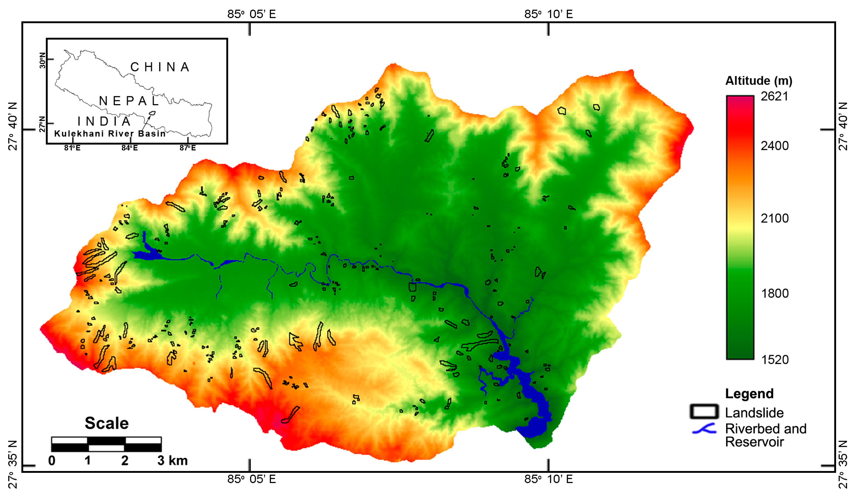
The Kulekhani River Basin in Central Nepal is selected as a test case. The basin is located about 30 km southwest of Kathmandu in the Bagmati province of Nepal, as shown in Figure 1. The total area is 124.26 km2 and contains the 1.24 km2 Kulekhani Reservoir in the southeast, which supports three hydroelectric power stations that are of vital importance to Nepal. The basin consists of uneven terrain with steep hills and narrow valleys, and altitudes ranging from 1520 m to 2621 m, as shown in Figure 1. The geology of the area includes Proterozoic and Paleozoic rocks, mainly schist, quartzite, sandstone, siltstone, and shale, and intrusive Palung Granite in the southern part of the basin [31,32,33,34]. The basin is characterized by two climatic zones: a warm temperate humid zone below 2000 m with average temperatures of 15–20 °C and a cool temperate humid zone above 2000 m with average temperatures of 10–15 °C and snowfall in the winter season. The average annual rainfall is about 1600 mm, most of which falls in the monsoon season from June to September. The basin is drained by the Kulekhani River, which empties into the Kulekhani Reservoir. The river system is mainly rain-fed and perennial, while upper channels are ephemeral and can be very destructive in the rainy season.
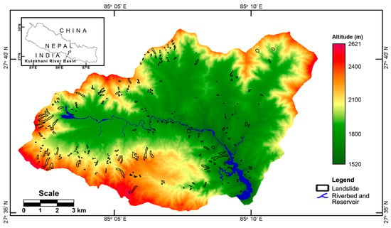
Figure 1.
Location map of the Kulekhani River Basin in Central Nepal, indicating topography, riverbed and reservoir, and observed landslides.
Several researchers have studied rainfall-induced landslides in this basin, e.g., [35,36,37,38,39,40]. All spatially referenced data relevant to this study are taken from Kayastha et al. [40]. As the focus of the present study is on the methodology for landslide susceptibility assessment, only a brief description of the data is provided, as more details can be found in the original study [40].
The landslide inventory is based on aerial photographs and digital maps of the Survey Department of the Government of Nepal and verified by field surveys [39]. As many as 295 landslides were identified, as shown in Figure 1, including debris slides, soil slides, rockslides, plane and wedge failures, and rotational slides, ranging in size from about 400 m2 to 0.1 km2. The landslides cover in total an area of 2.35 km2, which is 1.9% of the total study area. The prior unconditional landslide probability is therefore .
The digital elevation model of the study area, shown in Figure 1, with a cell size of 20 × 20 m2 was derived from digital elevation contours with intervals of 20 m obtained from the Survey Department of the Government of Nepal. From this map, geomorphological thematic data layers were derived, such as slope aspect, angle, shape, curvature, and relative relief. A slope map was generated showing six classes: flat to gentle (<5°), fair (5–15°), fairly moderate (15–25°), moderate (25–35°), steep (35–45°), and very steep (>45°). The slope aspect was divided into nine classes: four cardinal directions, four intercardinal directions, and flat terrain. Slope curvature was divided into three classes: convex, planar (straight), and concave. Relative relief, computed as the difference between maximum and minimum altitudes per hectare of land, was divided into four classes: <25 m/ha, 25–50 m/ha, 50–100 m/ha, and >100 m/ha.
The land use map was prepared by the Survey Department of the Government of Nepal. Nine classes of land use are identified: built-up area, agricultural land, forest, plant nursery, grassland, bush, riverbed, barren land and reservoir, as shown in Figure 2.
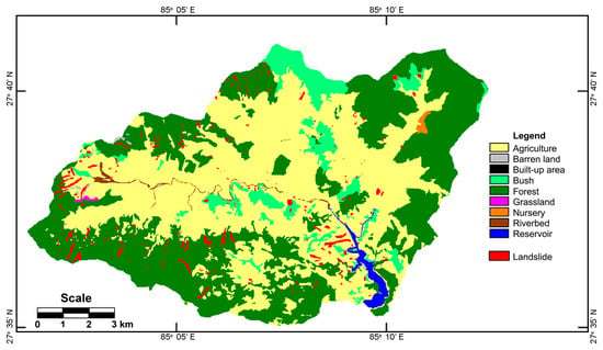
Figure 2.
Map of the Kulekhani River Basin, showing the land use and observed landslides.
Two hydrologic factors were considered. The influence of runoff on landslides was evaluated using the distance to drainage axes, grouped into four classes: <25 m, 25–50 m, 50–100 m, and >100 m. The effect of rainfall as a trigger for landslides was taken into account by long-term annual rainfall, grouped into three classes: <1500 mm/y, 1500–1750 mm/y, and >1750 mm/y.
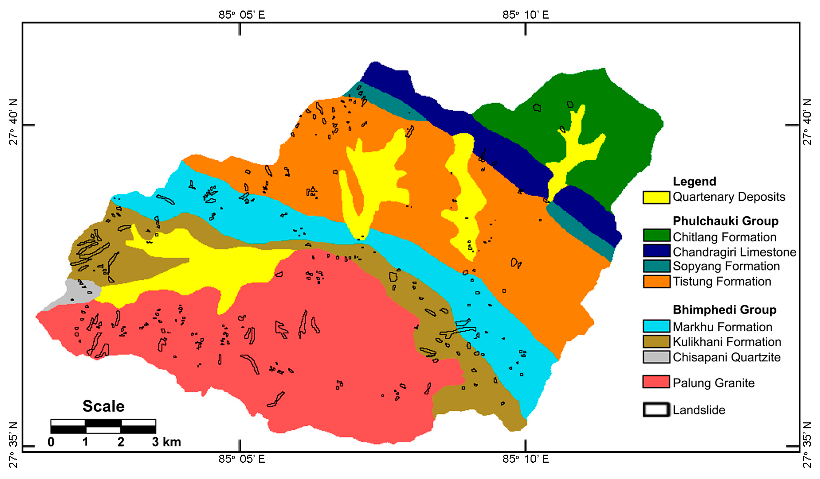
The geological map shown in Figure 3 was derived based on the geological maps presented by Stöcklin and others [31,32,33,34]. The Chisapani Quartzite is the oldest formation in the basin and is followed by the Kulikhani Formation (schist and quartzite) and Markhu Formation (schist, quartzite, and marble) of the Bhimphedi Group. The succeeding Phulchauki Group begins with the Tistung Formation (sandstone and siltstone) and passes into the overlying Sopyang Formation (slate and limestone), Chandragiri Limestone and Chitlang Formation (slate). The Palung Granite is distributed only in the southern part of the basin, and Quaternary sediments are confined to the major river valleys.
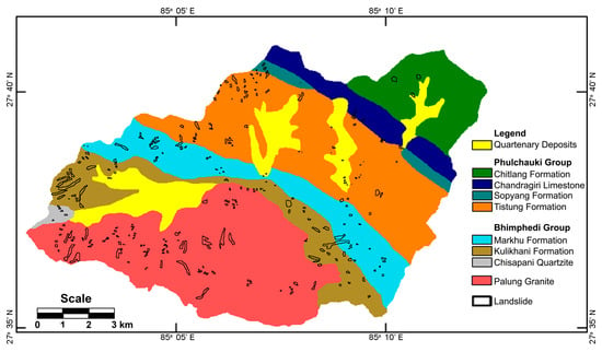
Figure 3.
Geological map of the Kulekhani River Basin, modified from [31,32,33].
3. Results
3.1. Naïve Bayes Model
Weights-of-evidence results are obtained using the R Information package [41]. The results are presented in Table 2. The value expresses the predictive strength of a factor class for landslide occurrence with respect to the prior probability. If is positive, the posterior probability of a landslide is greater than the prior probability, and vice versa. Positive values, therefore, indicate greater landslide susceptibility. Extreme values of weights-of-evidence indicate that the factor class is highly significant for predicting landslides, while values close to zero show that the factor class has little or no effect on landslide occurrence.

Table 2.
Results obtained from weights-of-evidence: factors and classes, probabilities and of factor class present or absent in case of landslides, and resulting weight and information value .
The results of the weights-of-evidence indicate that the landslide probability is higher than average on northeast and easterly facing slopes and lower than average on flat, west, and southwesterly facing slopes. Obviously, this is due to the prevailing direction of the monsoon storms that enter from the east and slowly move westward while producing heavy rainfall. The IVs show that these slope aspect classes have a weak predictive power for landslides, while the other classes of slope aspect have no predictive power.
For slope angle, the weights generally increase with increasing slope angle. Flat to gentle slopes are expected to have a low risk of landslides, while steep to very steep slopes are highly susceptible to landslides. Table 2 shows that for slope angles smaller than 25°, weights are negative, indicating a lower-than-average probability for landslide occurrence, and for slope angles above 25° weights are positive, indicating a higher-than-average landslide probability. The corresponding IVs show that all slope angle classes have weak to medium predictive power, except the middle group, 15–25°, which has no predictive power because the posterior probability is not significantly different from the prior probability.
For the slope shape, the weight is positive for convex and concave slopes and negative for straight slopes. A likely explanation is that convex or concave slopes retain more water after heavy rainfall, increasing groundwater pressures and reducing shear resistance [42]. However, the IVs show that only straight slopes have a weak predictive power, and convex and concave slopes have no predictive power, implying that the landslide probability for these slopes is only average.
For the relative relief, the weight is positive for the 50–100 m/ha class and negative for the other classes. The IVs show that the 50–100 m/ha class has only weak predictive power, while the <25 m/ha class has medium predictive power, and for other classes, the predictive power is insignificant. These results are somewhat similar to what is obtained for the slope angle, i.e., flatter terrain impedes landslides while steeper terrain favors landslides or results in a medium landslide probability.
Drainage distance has a clear influence on landslides: the closer to a drainage axis, the greater the weight. At less than 25 m, the weight is positive, while at a distance more than 25 m, the weight is negative and clearly continues to decrease with distance, indicating a lower probability of landslides farther from rivers. All classes are of weak or medium predictive power except for the 25–50 m class. These results may be related to weak riverbanks and the destructive power of river currents.
In the case of landslides and geology, the weights are positive for the Kulekhani Formation, Palung Granite, Chisapani Quartzite, and Markhu Formation, while negative for the Tistung Formation, Sopyang Formation, Chitlang Formation, Chandragiri Limestone, and Quaternary deposits. The predictive power is medium for the Kulekhani Formation and Quaternary deposits and weak for the other classes, with the exception of Chisapani Quartzite and Markhu Formation, which show no predictive power. Thus, it appears that the probability of landslides is higher for the older and more weathered formations, i.e., the Proterozoic Kulikhani Formation and Markhu Formation, that are composed of flaky minerals that weather easily, and lower for the younger Paleozoic formations, i.e., the Tistung Formation, Sopyang Formation, Chandragiri Limestone and Chitlang Formation, which consisting mainly of slate, sandstone, and limestone. In addition, the intrusive Palung Granite in the south of the study area is known to be highly weathered and very vulnerable to landslides [36,37,38], while the Quaternary deposits in the valleys are generally more resistant to slope failure [38].
The influence of land use is also very clear, as the weights are positive for forest, grassland, bush, and barren land and negative for agricultural land and riverbeds. For built-up areas, plant nurseries, and the reservoir, the weights are set equal to zero because no landslides have been observed in these classes. Hence, these are treated as missing data, which is the standard procedure in the R Information package. However, the IVs indicate that the predictive power is only weak for agricultural land, forest, and barren land and negligible for all other land uses.
There is a clear relationship between landslide occurrence and annual rainfall, as the weight is positive for areas with more than 1750 mm of precipitation per year and negative otherwise. The IVs indicate weak predictive power for the classes with less rainfall than 1750 mm/y and medium predictive power for the classes with rainfall larger than 1750 mm/y.
The total IVs for the causative factors are presented in Table 3. The IVs are ranked from highest to lowest. Note that these values are significantly larger than the IVs obtained for the factor classes, given in Table 2, obviously because they are obtained by adding the IVs for all classes belonging to a factor. Geology has the highest score and is the only factor with very strong predictive power. This is a surprise because the IVs for the individual geology class indicate only medium or less predictive. The much better overall score is clearly due to the large number of classes. Therefore, while any class may have a low impact, the combination of all classes becomes much better, as more classes imply more diversity and contrast, resulting in a greater predictive power. Relative relief is the second most important factor with strong predictive power. There are only four classes in this factor, but one of them, i.e., class < 25 m/ha, already has medium, almost strong predictive strength. All other factors have medium to weak predictive power, hence, no factor is unimportant. Application of landslide susceptibility assessment in the Kulekhani River Basin presented by Dhakal et al. [36,37] and Dhital [38] also concluded that geology is the main causative factor for landslide susceptibility in the Kulekhani River Basin.

Table 3.
Information values for the factors and evaluation of the predictive strength.
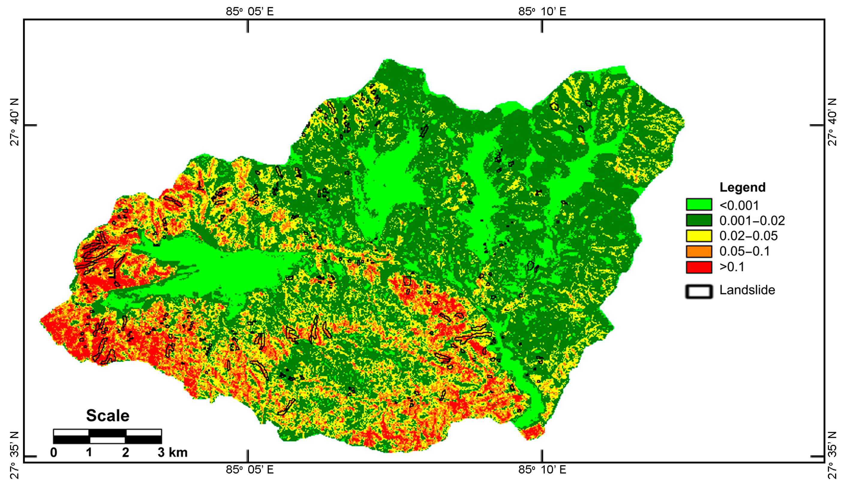
A map of the posterior probability, , obtained using Equation (6) and taking the inverse of the logit-function, is shown in Figure 4. The resulting values range from zero to 0.81. Since the values are very skewed, categories have been devised accordingly. The green colors represent posterior probabilities that are smaller than the prior probability, which is rounded to 0.02 for clarity, so these are zones less prone to landslides. The other colors represent the opposite, posterior probabilities that are greater than the prior probability, i.e., zones prone to landslides. The category shown in red represents posterior probabilities larger than 0.1, covering a large part of the southeast of the basin.
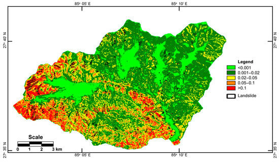
Figure 4.
Posterior landslide probability map of the Kulekhani River Basin obtained from the naïve Bayes weights-of-evidence model, given by Equation (6).
3.2. Semi-Naïve Bayes Model
The results of the semi-naïve Bayes model are derived by logistic regression with weights-of-evidence as variables. The logistic regression coefficients are estimated by fitting the model to the observed landslides using maximum likelihood with the glm generalized maximum likelihood fitting procedure of the R stats package for statistical computing [43].
The results of the logistic regression are shown in Table 4. The table lists the estimates of the regression coefficients and the corresponding standard error, the test statistics (z-value), and the significance test (Pr (>|z|)). All estimates of the logistic regression coefficients are highly significant, except for the slope shape, which is not significant. Note that the estimated intercept, , is very close to the logit of the prior landslide probability, , and that all estimated regression coefficients for the factors are less than one, resulting in smaller values for the posterior landslide probabilities than obtained from weights-of-evidence.

Table 4.
Results of the logistic regression: factors, logistic regression coefficients, estimates for the regression coefficients, standard deviation of the predicted values, z-statistic, and probability test of the z-score (Pr (>|z|)).
The results of the logistic regression show that the factors with more predictive power, geology, relative relief, and drainage distance are moderately corrected with values in the range of 0.7 to 0.9, factors with less predictive power, slope angle, slope aspect, annual rainfall, and land use are much more corrected with values in the range of 0.2 to 0.7, and the factor with very little predictive power, slope shape, is virtually removed from the model.
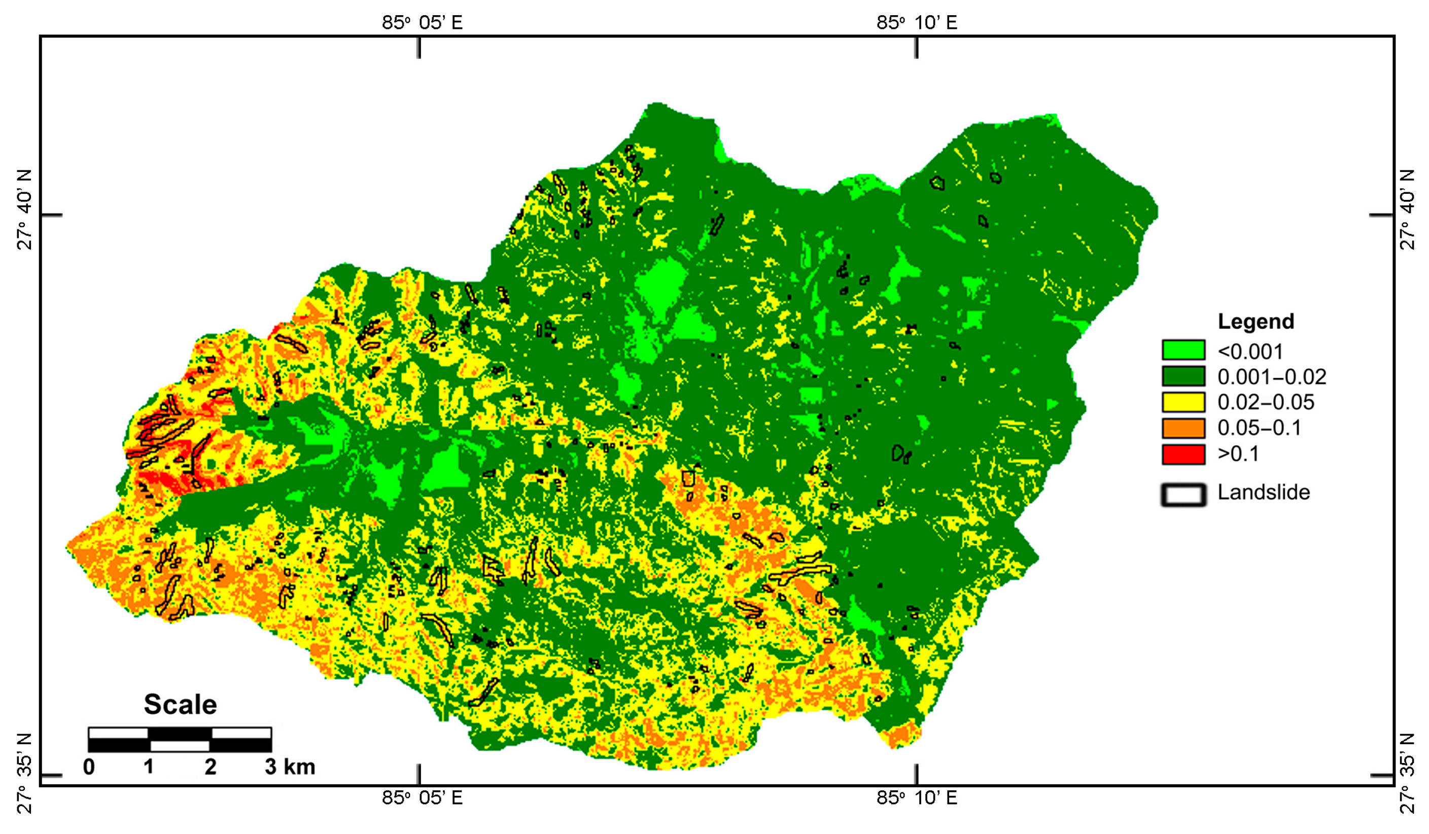
A map of the posterior probability , obtained using Equation (10) and taking the inverse of the logit-function, is shown in Figure 5. The resulting values vary from zero to 0.37. Since the values are also very skewed, the same categories are used as in Figure 4. It is noticeable that there are many more areas with posterior probabilities smaller than the prior probability, and vice versa, compared to Figure 4.

Figure 5.
Posterior landslide probability map of the Kulekhani River Basin obtained from the semi-naïve Bayes logistic regression with weights-of-evidence model, given by Equation (10).
4. Discussion
Comparison of Figure 4 and Figure 5 shows clear differences between the size and distribution of the posterior probabilities obtained from the naïve Bayes and semi-naïve Bayes models. Questions that need to be answered are whether there is bias involved and which method provides the most discriminatory power for landslide susceptibility mapping.
Bias can be determined by comparing the mean posterior probability to the prior observed landslide probability. It turns out that the mean of the posterior probability obtained from the naïve Bayes classification using weights-of-evidence is 0.027, while for the semi-naïve Bayes classification using logistic regression with weights-of-evidence, it becomes 0.019, which exactly matches with the observed prior probability . Thus, the weights-of-evidence results are strongly biased, while the results after correction by logistic regression are unbiased. This is further demonstrated by comparing the mean posterior probabilities for the 295 observed landslides in the study area. Figure 6 shows a plot of the posterior probabilities of the observed landslides derived from the naïve and semi-naïve Bayes models. The posterior probability values obtained from weights-of-evidence are markedly larger, almost double, than the values obtained from logistic regression combined with weights-of-evidence. Hence, the bias of the weights-of-evidence method gives a false impression of the true probability of a landslide.
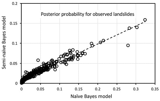
Figure 6.
Posterior probabilities for the 295 observed landslides obtained from the naïve and semi-naïve Bayes models.
The discriminatory power of the posterior probabilities obtained from both methods is assessed by receiving the operating characteristic (ROC) and area under the curve (AUC), which are standard techniques to evaluate the performance of classification models. The ROC curve is obtained by varying a threshold for the landslide probability and plotting the true positive rate, i.e., the fraction of observed landslide areas with a predicted posterior probability greater than the threshold, against the false positive rate, being the fraction of landslide-free areas and a predicted posterior probability greater than the threshold. The resulting ROC curves are shown in Figure 7. The two ROC curves are very close to each other, but the semi-naïve Bayes model is slightly above the curve for the naïve Bayes model. The corresponding AUC values are 0.77 and 0.76 for the semi-naïve Bayes model and naïve Bayes model, respectively. Thus, both models have nearly equal discriminatory power for landslide susceptibility mapping, which may seem strange because the naïve Bayes posterior probabilities are biased. However, the bias of the naïve Bayes model is consistent, so this has little effect on discriminatory power because only differences are important and not absolute values. In such a case, AUC and ROC are mainly determined by the quality and quantity of the data and less by the accuracy of the model. Nevertheless, thresholds for landslide susceptibility mapping in the case of naïve Bayes modeling will have little physical meaning due to the bias, although they may be useful for classification purposes.
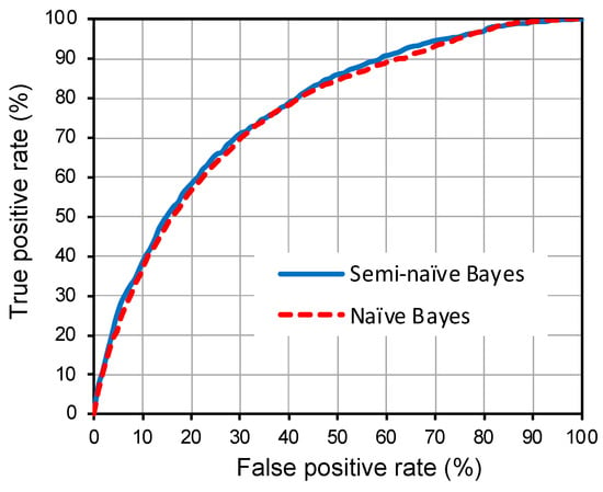
Figure 7.
ROC curves obtained from the naïve Bayes and semi-naïve Bayes classification models.
For completeness, we also derived contrast values with weights-of-evidence as suggested by Bonham-Carter [14] and obtained an AUC value of 0.75, which is slightly lower than what is obtained from the naïve and semi-naïve approaches used in this study. So, although the contrast is likely biased as well, it can be useful for the classification of landslide susceptibility. In a previous study, Kayastha et al. [40] applied one heuristic and two statistical bivariate methods for landslide susceptibility mapping in the Kulekhani River Basin. The heuristic method was less accurate, which may be attributed to weights assigned based solely on expert judgment, but the two statistical methods yielded identical results with an AUC value of 0.76. Though all methods are usable for classification purposes, the semi-naïve Bayes model proposed in this study is unbiased and, hence, most meaningful.
The results obtained from the semi-naïve Bayes model are preferred for landslide susceptibility classification because they are unbiased. However, the posterior probability is not very practical for classification because the distribution over the study area is very skewed, as can be seen in Figure 5. Therefore, it is more practical to use the logit transformed probability given by Equation (10), and since the intercept is just a constant, it can be subtracted so that we obtain as the most suitable classifier. Therefore, a landslide susceptibility index (LSI) is defined as
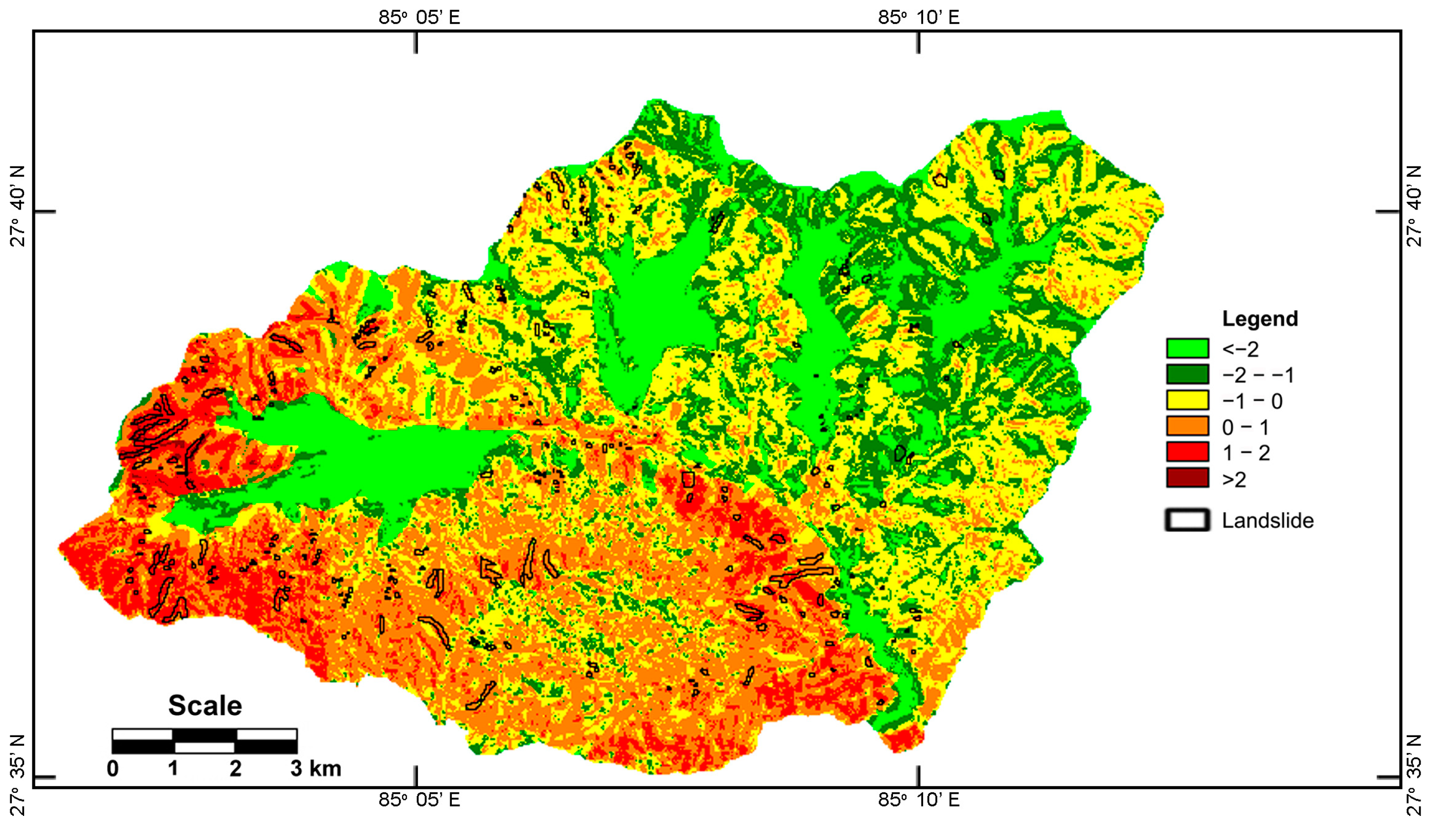
Positive LSI values correspond to posterior landslide probabilities greater than the prior landslide probability, thus indicating landslide-prone areas, and conversely, negative LSI-values indicate areas less susceptible to landslides. Note that the logit transform and subtraction of the intercept have no effect on the discriminatory power, so LSI has the same ROC and AUC as for the semi-naïve Bayes model, as shown in Figure 7. The LSI values are obtained using the predict function of the R stats package [43]. Uncertainty in the LSI values is also obtained as the standard error of the predictions using the se.fit argument of the predict function. The standard errors take into account the standard deviation of the residuals obtained after fitting the model to the observations and the standard deviation of the predicted model coefficients, shown in Table 4. The predicted values and standard errors of LSI are shown in Figure 8 and Figure 9.

Figure 8.
Index map for the landslide susceptibility of the Kulekhani River Basin obtained from the semi-naïve Bayes logistic regression with weights-of-evidence model, given by Equation (11).
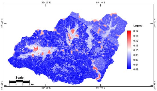
Figure 9.
Standard error map of the Kulekhani River Basin obtained from the semi-naïve Bayes logistic regression with weights-of-evidence model, given by Equation (11).
The LSI values vary between −7.18 and 3.13. The values can be divided into categories that allow us to classify the study area into different landslide susceptibility zones. In practice, there is no straightforward rule to automatically categorize LSI values. Most researchers use expert opinion to develop classes that conform to the principle that zones of greater landslide susceptibility correspond to more landslide occurrences. Some studies establish fixed percentages of observed landslides or fixed percentages of area covered to derive such categories. However, such classifications are subjective. Therefore, in this study, we use the LSI values on their own merits without fixing the percentages of observed landslides or covered areas. The thresholds from −2 to 2 in increments of 1 are used to define six susceptibility zones, as shown in Table 5. We also avoid naming the susceptibility zones, such as high susceptibility and the like, because this is also subjective.

Table 5.
Landslide susceptibility zones in the Kulekhani River Basin: category number, LSI value, percentage of total area, percentage of observed landslides, and the ratio of landslides and area percentages.
Table 5 lists the percentages of the total area and of the observed landslides per landslide susceptibility class as well as the frequency ratio between these percentages. There appears to be a reasonable agreement between the resulting landslide susceptibility zones, shown in Figure 8, and the observed landslide inventory, shown in Figure 1. Landslides are generally observed in areas with high LSI values, but the agreement is obviously not perfect. The results show that 76.1% of the landslides occurred in areas with LSI-values larger than zero, covering 36.8% of the study area. There is also a clear upward trend of the frequency ratio with increasing LSI. The ratio is smallest for zone 1, which largely corresponds to Quaternary deposits in valleys least subject to landslides. Zones 2 and 3 have slightly higher frequency ratios and consist mainly of the less weathered formations of the Phulchauki Group in the northeast of the study area. Zones 4 and 5 have frequency ratios greater than one and contain mainly the more weathered formations of the Bhimphedi Group and the heavily weathered intrusive Palung Granite in the southwest of the study area. These zones, which represent about 37% of the basin, are therefore more vulnerable to landsliding. The last zone, Zone 6, is very small, about 0.2% of the basin, but has a very high-frequency ratio and largely coincides with a series of landslides in the western corner of the basin. Overall, the predictive power of the landslide susceptibility map is thus quite significant.
The standard error of the predicted LSI values, shown in Figure 9, ranges from 0.02 to 0.17. This means that the deviation of the LSI values can be estimated to be 1.96 times the standard error or about 0.04 to 0.33. However, for most of the study area, the standard error is less than 0.08, so the deviation is less than 0.16. The higher deviations are concentrated in the valleys and can clearly be associated with large negative LSI values. Obviously, the greater the absolute LSI value, the greater the error will be.
5. Conclusions
Naïve Bayes and semi-naïve Bayes methods were presented for landslide susceptibility analysis. It is shown that the naïve Bayes model based on weights-of-evidence can be biased in case the independence conditions between causative factors are not met, resulting in an overprediction of the posterior landslide probabilities. Therefore, a semi-naïve Bayes approach is proposed using logistic regression with weights-of-evidence, which proves to be unbiased and, therefore, predicts unbiased posterior landslide probabilities that can be used for landslide susceptibility mapping.
The usefulness of the proposed methodology was demonstrated by assessing landslide susceptibility in the Kulekhani River Basin, Nepal. The results show that the naïve Bayes weights-of-evidence overpredicts the posterior landslide probability by a factor of two, while the semi-naïve Bayes approach, which uses logistic regression with weights-of-evidence, is unbiased and has greater discriminatory power for landslide susceptibility mapping, as revealed by the receiving operating characteristics. Furthermore, the semi-naïve Bayes approach enables us to statistically identify the main causative factors that promote landslides.
An appropriate landslide susceptibility index was proposed using the logit transformed posterior probability obtained from the semi-naïve Bayes model. The resulting LSI values can derive landslide susceptibility zones that are not subjective to personal judgment and appear to be consistent with the observed landslide inventory. The semi-naïve Bayes model also allows us to derive the model uncertainty of the predicted landslide susceptibility by calculating the standard error of the predictions.
Author Contributions
Conceptualization, F.D.S. and P.K.; methodology, F.D.S. and P.K.; software, F.D.S.; validation, F.D.S. and P.K.; formal analysis, F.D.S. and P.K.; investigation, P.K. and M.R.D.; resources, P.K. and M.R.D.; data curation, P.K. and M.R.D.; writing—original draft preparation, F.D.S.; writing—review and editing, F.D.S., P.K., and M.R.D.; visualization, P.K.; supervision, F.D.S.; project administration, F.D.S. All authors have read and agreed to the published version of the manuscript.
Funding
This research received no external funding.
Data Availability Statement
Not applicable.
Acknowledgments
The authors would like to thank Gautam Prasad Khanal, Department of Mines and Geology, Government of Nepal, for his assistance with the map projection used by the Department of Mines and Geology, Government of Nepal.
Conflicts of Interest
The authors declare no conflict of interest.
References
- Wickramasinghe, I.; Kalutarage, H. Naive Bayes: Applications, variations and vulnerabilities: A review of literature with code snippets for implementation. Soft. Comput. 2021, 25, 2277–2293. [Google Scholar] [CrossRef]
- Zaidi, N.A.; Cerquides, J.; Carman, M.J.; Webb, G.I. Alleviating naive Bayes attribute independence assumption by attribute weighting. J. Mach. Learn. Res. 2013, 14, 1947–1988. [Google Scholar]
- Guzzetti, F.; Reichenbach, P.; Cardinali, M.; Galli, M.; Ardizzone, F. Probabilistic landslide hazard assessment at the basin scale. Geomorphology 2005, 72, 272–299. [Google Scholar] [CrossRef]
- Wu, W.; Sidle, R.C. A distributed slope stability model for steep forested basins. Water Resour. Res. 1995, 31, 2097–2110. [Google Scholar] [CrossRef]
- Dai, F.C.; Lee, C.F.; Xu, Z.W. Assessment of landslide susceptibility on the natural terrain of Lantau Island, Hong Kong. Env. Geol. 2001, 40, 381–391. [Google Scholar] [CrossRef]
- Dahal, R.K.; Hasegawa, S.; Nonomura, A.; Yamanaka, M.; Dhakal, S.; Paudyal, P. Predictive modeling of rainfall-induced landslide hazard in the Lesser Himalaya of Nepal based on weights-of-evidence. Geomorphology 2008, 102, 496–510. [Google Scholar] [CrossRef]
- Huabin, W.; Gangjun, L.; Gonghui, W. GIS-based landslide hazard assessment: An overview. Prog. Phys. Geog. 2005, 29, 548–567. [Google Scholar] [CrossRef]
- Van Westen, C. Statistical Landslide Hazard Analysis ILWIS 21 for Windows Application Guide; ITC Publication: Enschede, The Netherlands, 1997; pp. 73–84. [Google Scholar]
- Lee, S.; Choi, J.; Min, K. Landslide susceptibility analysis and verification using the Bayesian probability model. Env. Geol. 2002, 43, 120–131. [Google Scholar] [CrossRef]
- Lee, S. Current and future status of GIS-based landslide susceptibility mapping: A literature review. Korean J. Remote Sens. 2019, 35, 179–193. [Google Scholar] [CrossRef]
- Reichenbach, P.; Rossi, M.; Malamud, B.D.; Mihir, M.; Guzzetti, F. A review of statistically-based landslide susceptibility models. Earth Sci. Rev. 2018, 180, 60–91. [Google Scholar] [CrossRef]
- Rossi, M.; Guzzetti, F.; Reichenbach, P.; Mondini, A.C.; Peruccacci, S. Optimal landslide susceptibility zonation based on multiple forecasts. Geomorphology 2010, 114, 129–142. [Google Scholar] [CrossRef]
- Bonham-Carter, G.F.; Agterberg, F.P.; Wright, D.F. Weights of evidence modeling: A new approach to mapping mineral potential. In Statistical Applications in the Earth Sciences; Agterberg, F.P., Bonham-Carter, G.F., Eds.; GSC-89-9; Geological Survey: Ottawa, ON, Canada, 1989; pp. 171–183. [Google Scholar]
- Bonham-Carter, G.F. Geographic Information Systems for Geoscientists; Pergamon: Oxford, UK, 1994; 398p. [Google Scholar]
- Zhang, D.; Agterberg, F. Modified weights-of-evidence modeling with example of missing geochemical data. Complexity 2018, 2018, 7945960. [Google Scholar] [CrossRef]
- Van Westen, C.J.; Rengers, N.; Soeters, R. Use of geomorphological information in indirect landslide susceptibility assessment. Nat. Hazards 2003, 30, 399–419. [Google Scholar] [CrossRef]
- Neuhäuser, B.; Terhorst, B. Landslide susceptibility assessment using “weights-of-evidence” applied to a study area at the Jurassic escarpment (SW-Germany). Geomorphology 2007, 86, 12–24. [Google Scholar] [CrossRef]
- Regmi, N.R.; Giardino, J.R.; Vitek, J.D. Modeling susceptibility to landslides using the weight of evidence approach: Western Colorado, USA. Geomorphology 2010, 115, 172–187. [Google Scholar] [CrossRef]
- Cervi, F.; Berti, M.; Borgatti, L.; Ronchetti, F.; Manenti, F.; Corsini, A. Comparing predictive capability of statistical and deterministic methods for landslide susceptibility mapping: A case study in the northern Apennines (Reggio Emilia Province, Italy). Landslides 2010, 7, 433–444. [Google Scholar] [CrossRef]
- Chen, X.; Chen, H.; You, Y.; Chen, X.; Liu, J. Weights-of-evidence method based on GIS for assessing susceptibility to debris flows in Kangding County, Sichuan Province, China. Environ. Earth Sci. 2016, 75, 70. [Google Scholar] [CrossRef]
- Rahman, M.S.; Ahmed, B.; Di, L. Landslide initiation and runout susceptibility modeling in the context of hill cutting and rapid urbanization: A combined approach of weights of evidence and spatial multi-criteria. J. Mt. Sci. 2017, 14, 1919–1937. [Google Scholar] [CrossRef]
- Polykretis, C.; Chalkias, C. Comparison and evaluation of landslide susceptibility maps obtained from weight of evidence, logistic regression, and artificial neural network models. Nat. Hazards 2018, 93, 249–274. [Google Scholar] [CrossRef]
- Jaafari, A. LiDAR-supported prediction of slope failures using an integrated ensemble weights- of-evidence and analytical hierarchy process. Environ. Earth Sci. 2018, 77, 42. [Google Scholar] [CrossRef]
- Agterberg, F.P.; Cheng, Q. Conditional independence test for Weights-of-Evidence modelling. Nat. Resour. Res. 2002, 11, 249–255. [Google Scholar] [CrossRef]
- Deng, M. A conditional dependence adjusted weights of evidence model. Nat. Resour. Res. 2009, 18, 249–258. [Google Scholar] [CrossRef]
- Schaeben, H. A mathematical view of weights-of-evidence, conditional independence, and logistic regression in terms of markov random fields. Math. Geosci. 2014, 46, 691–709. [Google Scholar] [CrossRef]
- Agterberg, F. A modified weights-of-evidence method for regional mineral resource estimation. Nat. Resour. Res. 2011, 20, 95–101. [Google Scholar] [CrossRef]
- Siddiqi, N. Credit Risk Scorecards; John Wiley and Sons: Hoboken, NJ, USA, 2006. [Google Scholar]
- Larsen, K. Data Exploration with Weight of Evidence and Information Value in R. 2015. Available online: https://multithreaded.stitchfix.com/blog/2015/08/13/weight-of-evidence/ (accessed on 10 August 2023).
- Zhang, D.; Agterberg, F.; Cheng, Q.; Zuo, R. A comparison of modified fuzzy weights of evidence, fuzzy weights of evidence, and logistic regression for mapping mineral prospectivity. Math. Geosci. 2014, 46, 869–885. [Google Scholar] [CrossRef]
- Stöcklin, J.; Bhattarai, K.D. Geology of Kathmandu area and central Mahabharat Range, Nepal Himalaya. In HMG/UNDP Mineral Exploration Project, Technical Report; Department of Mines and Geology: Kathmandu, Nepal, 1977; 86p. [Google Scholar]
- Stöcklin, J. Geology of Nepal and its regional frame. J. Geol. Soc. 1980, 137, 1–34. [Google Scholar] [CrossRef]
- Regmi, M. Geology of Khulekhani Watershed in Central Nepal with Special Reference to Landslides and Weathering. Master’s Thesis, Tribhuvan University, Kirtipur, Kathmandu, Nepal, 2002. [Google Scholar]
- Dhital, M.R. Geology of the Nepal Himalaya; Springer: New York, NY, USA, 2015; 498p. [Google Scholar]
- Dhital, M.R.; Khanal, N.; Thapa, K.B. The Role of Extreme Weather Events, Mass Movements, and Land Use Changes in Increasing Natural Hazards; International Centre for Integrated Mountain Development: Kathmandu, Nepal, 1993; 108p. [Google Scholar]
- Dhakal, A.S.; Amada, T.; Aniya, M. Landslide hazard mapping and the application of GIS in the Kulekhani watershed, Nepal. Mt. Res. Dev. 1999, 19, 3–16. [Google Scholar] [CrossRef]
- Dhakal, A.S.; Amada, T.; Aniya, M. Landslide hazard mapping and its evaluation using GIS: An investigation of sampling schemes for a grid-cell based quantitative method. Photogramm. Eng. Remote Sens. 2000, 66, 981–989. [Google Scholar]
- Dhital, M.R. Causes and consequences of the 1993 debris flows and landslides in the Kulekhani watershed, central Nepal. In Debris-Flow Hazards Mitigation: Mechanics, Prediction, and Assessment; Rickenmann, D., Chen, C.L., Eds.; Millpress: Rotterdam, The Netherlands, 2003; pp. 931–942. [Google Scholar]
- Dhar, M.S.; Dhital, M.R. Application of Morishita Spread Index in the study of landslides from the Kulekhani watershed, central Nepal. J. Nepal Geol. Soc. 2004, 30, 123–126. [Google Scholar] [CrossRef]
- Kayastha, P.; Dhital, M.R.; De Smedt, F. Evaluation and comparison of GIS based landslide susceptibility mapping procedures in Kulekhani watershed, Nepal. J. Geol. Soc. India 2013, 81, 219–231. [Google Scholar] [CrossRef]
- Larsen, K. Information: Data Exploration with Information Theory (Weight-of-Evidence and Information Value). Available online: https://CRAN.R-project.org/package=Information (accessed on 12 August 2023).
- Lee, S.; Min, K. Statistical analysis of landslide susceptibility at Yongin, Korea. Env. Geol. 2001, 40, 1095–1113. [Google Scholar] [CrossRef]
- R Core Team. Team. R: A Language and Environment for Statistical Computing; R Foundation for Statistical Computing: Vienna, Austria. 2017; Available online: http://www.R-project.org/ (accessed on 15 November 2021).
Disclaimer/Publisher’s Note: The statements, opinions and data contained in all publications are solely those of the individual author(s) and contributor(s) and not of MDPI and/or the editor(s). MDPI and/or the editor(s) disclaim responsibility for any injury to people or property resulting from any ideas, methods, instructions or products referred to in the content. |
© 2023 by the authors. Licensee MDPI, Basel, Switzerland. This article is an open access article distributed under the terms and conditions of the Creative Commons Attribution (CC BY) license (https://creativecommons.org/licenses/by/4.0/).

