Comparative Evaluation of Empirical Approaches and Artificial Intelligence Techniques for Predicting Uniaxial Compressive Strength of Rock

Abstract

The uniaxial compressive strength (UCS) of rocks is one of the key parameters for evaluating the safety and stability of civil and mining structures. In this study, 386 rock samples containing four properties named the load strength (PLS), the porosity (P_n), the P-wave velocity (V_p), and the Schmidt hardness rebound number (SHR) are utilized to predict the UCS using several typical empirical equations (EA) and artificial intelligence (AI) methods, i.e., 16 single regression (SR) equations, 2 multiple regression (MR) equations, and the random forest (RF) models optimized by grey wolf optimization (GWO), moth flame optimization (MFO), lion swarm optimization (LSO), and sparrow search algorithm (SSA). The root mean square error (RMSE), determination coefficient (R²), Willmott’s index (WI), and variance accounted for (VAF) are used to evaluate the predictive performance of all developed models. The evaluation results show that the overall performance of AI models is superior to empirical approaches, especially the LSO-RF model. In addition, the most important input variable is the P_n for predicting the UCS. Therefore, AI techniques are considered as more efficient and accurate approaches to replace the empirical equations for predicting the UCS of these collected rock samples, which provides a reliable and effective idea to predict the rock UCS in the filed site.

1. Introduction

The uniaxial compressive strength (UCS) is one of the most important physical and–mechanical characteristic parameters of rock masses in civil and mining engineering design, which is also to be used for rock mass classification [1,2]. To date, the main accurate way to obtain the UCS is the direct laboratory method in the light of the International Society for Rock Mechanics (ISRM) and the American Society for Testing Materials (ASTM) [3]. However, the high-quality cores are necessary to obtain effective and reliable UCS in terms of the direct laboratory, and it is extremely difficult to obtain highly weathered rocks [1]. Furthermore, the complex operation, time-consuming aspects, and expensive equipment costs of the direct laboratory are often not considered into the UCS calculation in small- and medium-sized rock engineering projects. Therefore, it is a challenging and practical task for modern engineers to explore a convenient and accurate measurement method for rock UCS.

The empirical approaches are firstly developed by engineers and had achieved some good estimation results for estimating the rock UCS [4,5,6,7,8,9,10,11]. The empirical approaches are usually presented in the form of regression formulas, i.e., one or more parameters related to UCS are considered to establish deterministic equations for the UCS calculation. The results of the literature review showed that the porosity (P_n), the Schmidt hardness rebound number (SHR), the P-wave velocity (V_p), and the point load strength (PLS) are generally considered independent variables of the most of the empirical equations [3,8,9,12,13].

Nevertheless, the empirical formula universality is gradually exposed due to the limitation of sample location and lithology [14,15]. The same empirical formula is applied to different rock types while obtaining underestimates or overestimates for the UCS. Furthermore, the selection of independent variables depends largely on experienced engineers, which leads to objective errors. To eliminate the influence of lithology and the number and types of input parameters on the UCS estimation, numerous researchers have reported some successful cases in predicting the rock UCS by using different prediction models based on the artificial intelligence (AI) techniques, such as the artificial neural network (ANN) [16,17,18], the adaptive neuro-fuzzy inference system (ANFIS) [19,20], the support vector machine (SVM) [3,21,22], and the multi-layer perceptron (MLP) [20,23]. The random forest (RF) technique, with the advantages of anti-overfitting ability and processing the large amounts of data, is a common artificial intelligence model used to solve engineering prediction problems [24,25]. Many attempts have been tested to consider different metaheuristic optimization (MHO) algorithms to improve the performance of RF models, e.g., the imperialist competitive algorithm (ICA) [9,23], the particle swarm optimization (PSO) [12,17,25,26,27], the grey wolf optimization (GWO) [28,29], the artificial bee colony algorithm (ABC) [30], the firefly algorithm (FA) [31], multi-verse optimizer (MVO) [32], and the sine cosine algorithm (SCA) [33]. However, there are some algorithms that have not been applied to optimize the RF model for predicting the rock UCS (e.g., flame optimization (MFO), the lion swarm optimization (LSO), and the sparrow search algorithm (SSA)). In this study, four MHO algorithms are used to improve the performance of the RF models, i.e., GWO, MFO, LSO, and SSA. It should be noted that the hyperparameters of RF model and internal parameters of these MHO algorithms (e.g., number of trees (Nt) and the minimum sample number at a leaf node (Minlefsize) and the population in the MHO algorithms) are not easily understood and optimized compared to the parameters of empirical formulas [34].

In fact, mining engineers and geologists tend to use empirical approaches to estimate the UCS when the rock types have been identified. Furthermore, there are some novel intelligent models and optimization algorithms that have not been applied to the UCS prediction. Therefore, this study aims to compare the performance of empirical approaches and some novel AI models for predicting the rock UCS. To achieve this goal, various empirical equations are proposed as the representatives of empirical approaches, and four hybrid random forest (RF) models with different MHO optimization algorithms (i.e., GWO, MFO, LSO, and SSA) are developed and compared for the UCS prediction. A total of 386 rock samples are used to generate empirical equations and train MHO-RF models. Four statistical evaluation indices, i.e., the root mean square error (RMSE), the determination coefficient (R²), the Willmott’s index (WI), and the variance accounted for (VAF), are used to evaluate the performance of all the developed models.

2. Review the Related Works for Forecasting Rock UCS

The related work to forecast UCS of rock samples has been reviewed and presented comprehensively in this section, i.e., the application of empirical approaches (i.e., single and multiple regression formulas) and artificial intelligence models in the UCS prediction.

2.1. Existing Empirical Equations to Estimate UCS

The aim of the empirical approach is to reflect the mathematical relationship between the input parameters and the UCS. A small number of samples and simple experimental operations can be established to create a relationship between a single parameter (or multiple parameters) and the UCS, namely the single regression (SR) equation (multiple regression (MR) equation). Researchers have successfully predicted UCS by using a single factor to establish some similar SR equations (see Table 1), including the PLS, the P_n, the V_p, and the SHR. The PLS is usually used as the main parameter to predict the rock UCS, which can be obtained from the PLS tests at the rock engineering project site. Several researchers have reported a comprehensive list of empirical equations between the UCS estimation and the PLS [11,35,36]. The P_n can be estimated from physical tests for rock samples by using some simple and accurate experimental methods, such as the saturation and caliper techniques, the saturation and buoyancy techniques, etc. The V_p is determined through the ultrasonic pulse velocity (UPV) tests, which represent the compactness degree of the measured rock samples. The SHR is also an experimental parameter based on the Schmidt hammer, which indicates the strength of the tested materials. These four variables are widely used in the UCS estimation for different types of rocks in terms of establishing their respective SR equations [1,8,10,37,38].

Table 1. Related works on UCS prediction using the SR equations.

Variable	Single Equation	Samples	Lithologies	Reference
PLS	$\mathrm{UCS}=7.3{\mathrm{PLS}}^{1.71}$	188	sedimentary	Tsiambaos and Sabatakakis [39]
	$\mathrm{UCS}=10.52\mathrm{PLS}-3.966$	121	sedimentary	Yilmaz and Yuksek [19]
	$\mathrm{UCS}=16.4\mathrm{PLS}$	44	igneous	Kohno and Maeda [40]
	$\mathrm{UCS}=50.742{\mathrm{e}}^{0.2242\mathrm{PLS}}$	71	igneous	Armaghani et al. [9]
	$\mathrm{UCS}=17.6\mathrm{PLS}+13.5$	104	sedimentary	Aliyu et al. [11]
Pn	$\mathrm{UCS}=273.15{\mathrm{e}}^{0.076{\mathrm{P}}_{\mathrm{n}}}$	12	sedimentary	Palchik and Hatzor [41]
	$\mathrm{UCS}=-33.13{\ln (\mathrm{P}}_{\mathrm{n}})+64.6$	32	metamorphic	Diamantis et al. [42]
	$\mathrm{UCS}=228.2e^{-1.98{\mathrm{P}}_{\mathrm{n}}}$	20	sedimentary	Mishra and Basu [43]
	$\mathrm{UCS}=-287.7{\mathrm{P}}_{\mathrm{n}}+221.42$	71	igneous	Armaghani et al. [9]
	$\mathrm{UCS}={47.735\mathrm{P}}_{\mathrm{n}}{}^{-0.743}$	71	igneous	Armaghani et al. [10]
Vp	$\mathrm{UCS}=0.78{\mathrm{e}}^{0.88{\mathrm{V}}_{\mathrm{p}}}$	171	igneous	Entwisle et al. [44]
	$\mathrm{UCS}=0.11{\mathrm{V}}_{\mathrm{p}}-515.56$	32	metamorphic	Diamantis et al. [42]
	$\mathrm{UCS}=3.7{\mathrm{V}}_{\mathrm{p}}{}^{2.3}$	72	sedimentary	Beiki et al. [45]
	$\mathrm{UCS}=0.03{\mathrm{V}}_{\mathrm{p}}-53.709$	45	igneous	Armaghani et al. [9]
	$\mathrm{UCS}=18.506{\mathrm{e}}^{0.0003{\mathrm{V}}_{\mathrm{p}}}$	71	igneous	Armaghani et al. [9]
SHR	$\mathrm{UCS}=1.45{\mathrm{e}}^{0.07\mathrm{SHR}}$	40	igneous	Aydin and Basu [46]
	$\mathrm{UCS}=0.0137{\mathrm{SHR}}^{0.272}$	19	igneous, sedimentary metamorphic	Kılıç and Teymen [47]
	$\mathrm{UCS}=0.64\mathrm{SHR}+37.5$	29	igneous, metamorphic	Gupta [38]
	$\mathrm{UCS}=234.95\ln \left(\mathrm{SHR}\right)-799.521$	71	igneous	Armaghani et al. [9]
	$\mathrm{UCS}=8.36\mathrm{SHR}-416$	60	igneous, sedimentary metamorphic	Aladejare [1]

In addition, MR is another style of empirical approach developed by engineers and researchers to estimate the UCS [13,48,49,50,51,52]. The recent works of using MR on the UCS prediction are shown in Table 2. The main purpose of using MR equations is to estimate the UCS with multiple codependent variables. Diamantis et al. [42] only used the PLS and the V_p to create a good MR formula for estimating the UCS. Dehghan et al. [8] imposed a multivariate quadratic equation to calculate the UCS, which is different from the common equation (i.e., multivariate linear).

Table 2. Related works on UCS prediction using MR equations.

Variable	Multiple Equation	Samples	Lithologies	Reference
PLS, Vp, SHR	$\mathrm{UCS}=-35.9+0.89\mathrm{SHR}+13.4\mathrm{PLS}-1.68{\mathrm{V}}_{\mathrm{p}}$	90	igneous, sedimentary metamorphic	Karakus et al. [53]
PLS, Vp, SHR	$\mathrm{UCS}=4.14\mathrm{PLS}+29.8{\mathrm{V}}_{\mathrm{p}}+0.54\mathrm{SHR}-116$	15	sedimentary	Çobanoğlu and Çelik [48]
PLS, Vp	$\mathrm{UCS}=10.61\mathrm{PLS}+0.0687{\mathrm{V}}_{\mathrm{p}}-339.48$	32	metamorphic	Diamantis et al. [42]
PLS, Pn, Vp, SHR	$\begin{array}{l}\mathrm{UCS}=-442.363{\mathrm{V}}_{\mathrm{p}}+45.338{\mathrm{V}}_{\mathrm{p}}{}^2-6.1{\mathrm{P}}_{\mathrm{n}}+0.52{\mathrm{P}}_{\mathrm{n}}{}^2+28.31\mathrm{PLS}\\ -4.06{\mathrm{PLS}}^2+115.822\mathrm{SHR}-2.007{\mathrm{SHR}}^2-595.303\end{array}$	30	sedimentary	Dehghan et al. [8]
PLS, Vp	$\mathrm{UCS}=5.01\mathrm{PLS}+5.52{\mathrm{e}}^{0.0004{\mathrm{V}}_{\mathrm{p}}}-3.53$	85	igneous	Ng et al. [54]
PLS, Pn, Vp, SHR	$\mathrm{UCS}=-153.616{\mathrm{P}}_{\mathrm{n}}+7.111\mathrm{PLS}+0.01{\mathrm{V}}_{\mathrm{p}}+0.541\mathrm{SHR}+63.655$	71	igneous	Armaghani et al. [9]
PLS, Vp, SHR	$\begin{array}{l}\mathrm{UCS}=-35.051+11.442{\mathrm{e}}^{0.0297}\mathrm{SHR}+0.001{\mathrm{V}}_{\mathrm{p}}{}^{1.178}\\ +22.2971\mathrm{PLS}\end{array}$	124	igneous	Armaghani et al. [10]

2.2. Existing Artificial Intelligence Models for Estimating UCS

With the development of computer science and the popularity of interdisciplinary cross applications, numerous researchers have introduced AI models to predict the UCS and achieved remarkable results [1,12,15,55,56,57]. In this study, the PLS, the P_n, the V_p, and the SHR are considered as input variables in the UCS prediction, the related works have been shown in Table 3. Armaghani et al. [10] used the three nonlinear prediction models to forecast the UCS based on the 124 rock samples obtained from a tunnel in Malaysia. The results of predictive performance showed that the ANFIS has a better performance than the MR equations and ANN models. Furthermore, several studies have proved that the MHO optimization algorithms can improve the predictive performance of the initial AI models [58,59,60]. Momeni et al. [12] used the PSO algorithm to strengthen the performance of a BPNN model for predicting the UCS and achieved a success. Armaghani et al. [9] developed a hybrid model by combining the ANN and the ICA optimization algorithm to predict the UCS, and the results of prediction accuracy showed that the ANN performance has been significantly improved.

Table 3. Related works on UCS prediction using the AI models.

Variable	AI Models	Samples	Lithologies	Reference
PLS, Pn, Vp, SHR	ANN	30	sedimentary	Dehghan et al. [8]
PLS, Pn, Vp, SHR	PSO-BPNN	66	sedimentary, igneous	Momeni et al. [12]
PLS, Pn, Vp, SHR	ICA-ANN	71	igneous	Armaghani et al. [9]
PLS, Vp, SHR	ANFIS	124	igneous	Armaghani et al. [10]
PLS, Vp, SHR, BPI	FIS	108	sedimentary	Heidari et al. [13]
PLS, Pn, Vp, SHR	GPR	170	igneous, sedimentary, metamorphic	Mahmoodzadeh et al. [3]

Note: FIS: fuzzy inference system; GPR: Gaussian process regression; BPI: block punch index.

3. Rock Data Preparation and Performance Indices

To evaluate the performance of AI models and empirical approaches for predicting the UCS, more rock samples from various rock engineering projects with lithologic diversity were integrated to the rock database used in this study. As a result, a dataset of 386 rock samples was collected from different previously published research studies, including 30 Travertine samples from Haji mine by Dehghan et al. [8]; 71 Granite block rock samples from the PSRWT tunnel by Armaghani et al. [9]; 115 Granite samples of weathering Grade III from the bedrock in Macao, China by Ng et al. [54]; and 170 hybrid rock samples (Claystone, Granite, Schist, Sandstone, Travertine, Limestone, Slate, Dolomite, and Marl) from a quarry in Iran by Mahmoodzadeh et al. [3]. The above samples can be divided into three categories according to lithologies, i.e., igneous (Granite), sedimentary (Travertine, Claystone, Sandstone, Limestone, Dolomite, Marl), metamorphic (Schist, Slate). Reviewing the published studies, the P_n, the SHR, the V_p, and the PLS were also considered as input variables to predict the UCS; the statistical information of input and output variables according to the rock lithologies are shown in Table 4. As it can be seen in this table, the statistical values of the variables were similar for each rock lithology, indicating that the underlying relationship between four input variables and an output variable was consistent. Therefore, the rock data of different lithologies can be combined into a new database to improve the model prediction performance. Figure 1 shows the correlation between input and output variables based on different rock types. For the igneous rock data, the correlation between the V_p and the UCS was the greatest. The SHR had a stronger correlation with the UCS than other variables for both of sedimentary and metamorphic samples. Note that except the P_n, other three variables were positively correlated with the UCS. In general, correlation results directly illustrated the necessity for the above four variables with high correlation coefficient values to be considered as input variables for predicting the UCS.

Table 4. Details of input and output variables.

Lithologies	Variables	Types	Minimum	Maximum	Mean	Median	St. D
igneous	PLS (MPa)	input	0.89	11.73	4.08	3.97	1.76
	Pn (%)	input	0.10	7.23	1.48	0.98	1.51
	Vp (km/s)	input	1.16	7.94	4.76	4.70	1.19
	SHR	input	16.80	65.57	45.57	46.00	8.01
	UCS (MPa)	output	20.30	211.90	78.32	62.30	44.73
sedimentary	PLS (MPa)	input	0.89	14.13	3.98	3.29	2.33
	Pn (%)	input	0.06	16.80	3.53	0.54	4.28
	Vp (km/s)	input	2.73	7.61	5.35	5.47	0.95
	SHR	input	25.46	67.07	40.95	42.00	12.13
	UCS (MPa)	output	12.01	215.21	86.51	77.04	53.31
metamorphic	PLS (MPa)	input	0.86	9.08	4.58	3.72	2.09
	Pn (%)	input	0.12	14.67	3.58	1.54	4.06
	Vp (km/s)	input	2.99	7.94	5.24	5.23	0.96
	SHR	input	26.13	61.00	42.90	46.00	11.35
	UCS (MPa)	output	23.45	154.30	73.71	77.30	35.24
All samples	PLS (MPa)	input	0.86	14.13	4.07	3.57	2.04
	Pn (%)	input	0.06	16.80	2.49	0.85	3.32
	Vp (km/s)	input	1.16	47.94	5.04	5.09	1.12
	SHR	input	16.80	67.07	43.44	45.00	10.38
	UCS (MPa)	output	12.01	215.21	81.43	65.30	48.07

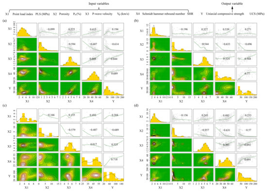
Figure 1. Correlation between input and output variables based on different rock types: (a) igneous; (b) sedimentary; (c) metamorphic; (d) all samples.

Four statistical evaluation indices were used to evaluate the performance of the empirical approaches and the proposed AI models, including the fact that the RMSE was responsible for measuring the difference between model predictions and observed values, the R² was used to judge the model fitting effect, and the WI was used to measure prediction accuracy and the VAF. The mean squared error (MSE) especially was considered separately as the fitness function to evaluate the optimization performance of all used MHO algorithms. These performance indices were introduced in several references [61,62,63,64,65,66,67,68,69] and are defined as follows:

$$\mathrm{RMSE}=\sqrt{\frac{1}{n}{\displaystyle \sum _{i=1}^n{\left(U_i-u_i\right)}^2}}$$

(1)

$$\mathrm{WI}=1-\left[\frac{{\displaystyle {\sum }_{i=1}^n{\left(U_i-u_i\right)}^2}}{{\displaystyle {\sum }_{i=1}^n{\left(\left|u_i-\overline{U}\right|+\left|U_i-\overline{U}\right|\right)}^2}}\right]$$

(2)

$$\mathrm{MSE}=\frac{1}{n}{\displaystyle \sum _{i=1}^n{\left(U_i-u_i\right)}^2}$$

(3)

$${\mathrm{R}}^2=1-\frac{{\left[{\displaystyle \sum _{i=1}^n(U_i-u_i)}\right]}^2}{{\displaystyle \sum _{i=1}^n{(u_i-\overline{u})}^2}}$$

(4)

$$\mathrm{VAF}=\left[1-\frac{\mathrm{var}(U_i-u_i)}{\mathrm{var}(U_i)}\right]\times 100\%,$$

(5)

where n is the number of the samples in the training and testing phase. U_i and u_i are the actual and predicted values of the UCS, respectively. $\overline{U}$ and $\overline{u}$ are the average of the actual values and the predicted values of the UCS, respectively.

4. Performance Evaluation of the Proposed Models in the UCS Estimation

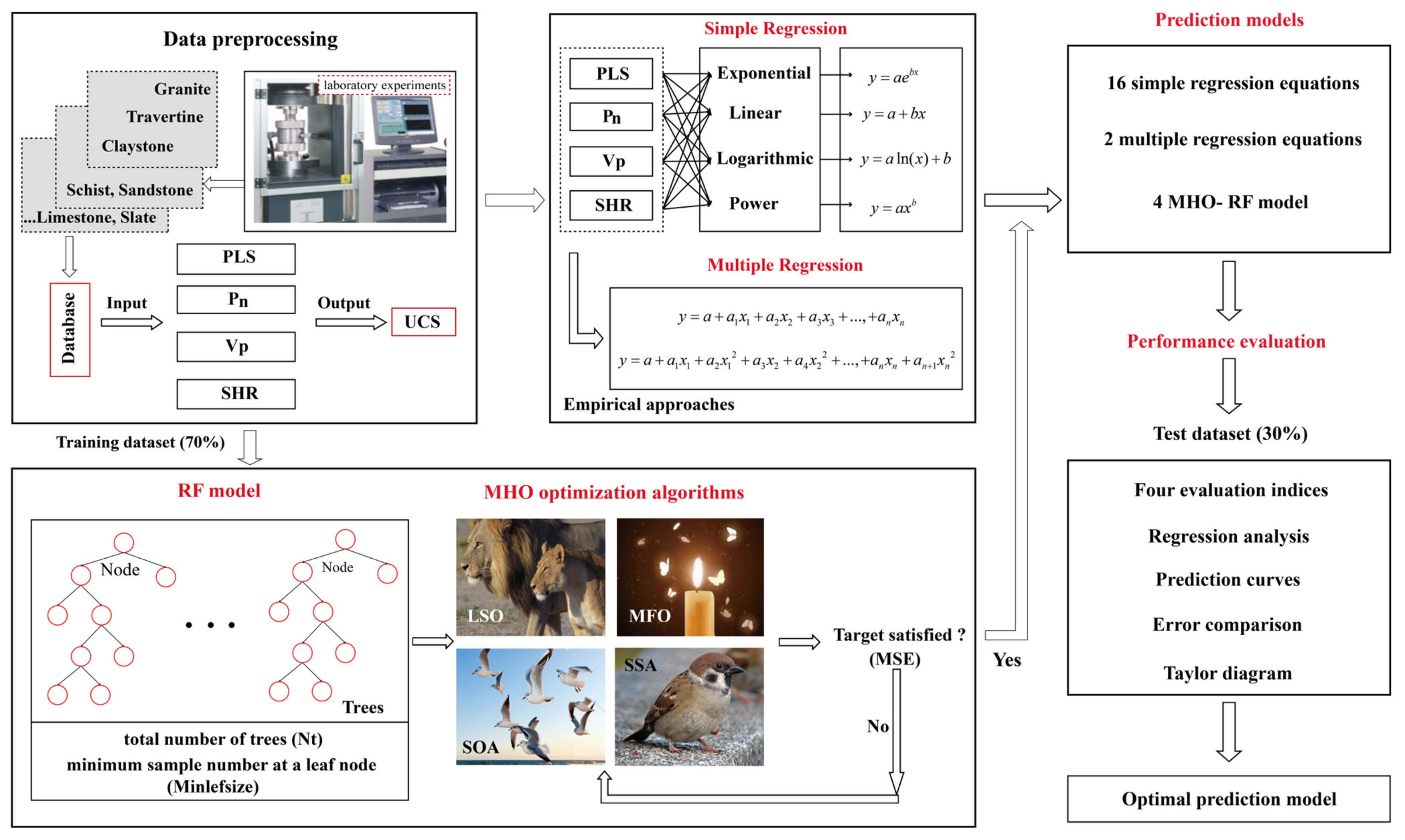
The 16 SR and 2 MR equations of empirical approaches and the other four hybrid MHO-RF (GWO-RF, MFO-RF, LSO-RF, and SSA-RF) models have been considered in this investigation. Figure 2 briefly displays a framework of the proposed methods in the UCS estimation and prediction. The development of the equations and models with their corresponding results are presented and discussed comprehensively.

Figure 2. Framework of predicting rock UCS based on the empirical approaches and artificial intelligence models.

4.1. Empirical Approaches

The SR analysis is the famous traditional method to estimate the rock UCS. In this study, four considered variables (PLS, P_n, V_p, and SHR) are established regression relationships with UCS, respectively. The form of the regression equation can be set to the exponential, linear, logarithmic, and power [9,54]. Table 5 shows the fitting results of all developed 16 SR equations on the UCS estimation. The values of R² and RMSE describe the performance of each single variable to predict the UCS with the whole data. For the exponential regression equation, the relationship between the V_p and the UCS is closer than others by result in higher value of R² and lower value of RMSE. From the power regression equation, the equation of P_n has a better performance in predicting the rock UCS.

Table 5. Results of single regression analyses for the UCS prediction.

Model	Regression Types	Variable	Function	R2	RMSE
SR-1	Exponential	PLS	$\mathrm{UCS}=47.523{\mathrm{e}}^{0.087\mathrm{PLS}}$	0.0483	48.3071
SR-2		Pn	$\mathrm{UCS}=90.99{\mathrm{e}}^{-0.119{\mathrm{P}}_{\mathrm{n}}}$	0.3356	39.1339
SR-3		Vp	$\mathrm{UCS}=10.28{\mathrm{e}}^{0.3738{\mathrm{V}}_{\mathrm{p}}}$	0.4748	34.7941
SR-4		SHR	$\mathrm{UCS}=9.6103{\mathrm{e}}^{0.449\mathrm{SHR}}$	0.4555	35.4278
SR-5	Linear	PLS	$\mathrm{UCS}=5.4924\mathrm{PLS}+59.084$	0.0544	46.6861
SR-6		Pn	$\mathrm{UCS}=-8.2588{\mathrm{P}}_{\mathrm{n}}+101.96$	0.3247	39.4528
SR-7		Vp	$\mathrm{UCS}=29.784{\mathrm{V}}_{\mathrm{p}}-68.775$	0.4792	34.6478
SR-8		SHR	$\mathrm{UCS}=3.199\mathrm{SHR}-57.547$	0.4773	34.7107
SR-9	Logarithmic	PLS	$\mathrm{UCS}=19.167\ln \left(\mathrm{PLS}\right)+56.909$	0.0419	46.9929
SR-10		Pn	$\mathrm{UCS}=-29.81{\ln (\mathrm{P}}_{\mathrm{n}})+83.676$	0.6676	27.6785
SR-11		Vp	$\mathrm{UCS}=123.19{\ln (\mathrm{V}}_{\mathrm{p}})-114.42$	0.4105	36.8604
SR-12		SHR	$\mathrm{UCS}=125.25\ln \left(\mathrm{SHR}\right)-387$	0.4529	35.5103
SR-13	Power	PLS	$\mathrm{UCS}=45.036{\mathrm{PLS}}^{0.3189}$	0.0465	48.6029
SR-14		Pn	$\mathrm{UCS}=69.772{\mathrm{P}}_{\mathrm{n}}{}^{-0.394}$	0.7222	25.3029
SR-15		Vp	$\mathrm{UCS}=5.208{\mathrm{V}}_{\mathrm{p}}{}^{1.6137}$	0.4315	36.1995
SR-16		SHR	$\mathrm{UCS}=0.0833{\mathrm{SHR}}^{1.7916}$	0.4591	35.3090

The purpose of MR analysis is to use appropriate variables for improving the computational accuracy. Most MR equations include two or more variables, but the forms of MR equations commonly used in the UCS prediction are mainly multivariate quadratic equations [8] and multivariate linear equations [9]. After determining the equation form, the coefficients can be calculated by using some fitting techniques, such as the least-squares fit. Therefore, two styles of MR equations are created through the four variables (PLS, P_n, V_p, and SHR) to predict the UCS as shown in Equations (6) and (7).

$${\mathrm{UCS}}_1=-119.786+3.831\mathrm{PLS}-1.048{\mathrm{P}}_{\mathrm{n}}+22.0009{\mathrm{V}}_{\mathrm{p}}+2.496\mathrm{SHR}$$

(6)

$$\begin{array}{cc}\hfill {\mathrm{UCS}}_2& =-28.2459-6.773\mathrm{PLS}+0.4437{\mathrm{PLS}}^2-8.7576{\mathrm{P}}_{\mathrm{n}}+0.5958{\mathrm{P}}_{\mathrm{n}}{}^2\hfill \\ & -7.112{\mathrm{V}}_{\mathrm{p}}+2.9622{\mathrm{V}}_{\mathrm{p}}{}^2+2.7389\mathrm{SHR}-0.0113{\mathrm{SHR}}^2\hfill \end{array},$$

(7)

where UCS₁ and UCS₂ represent the predicted UCS by using the multivariate linear of MR equation and multivariate-quadratic of MR equation, respectively.

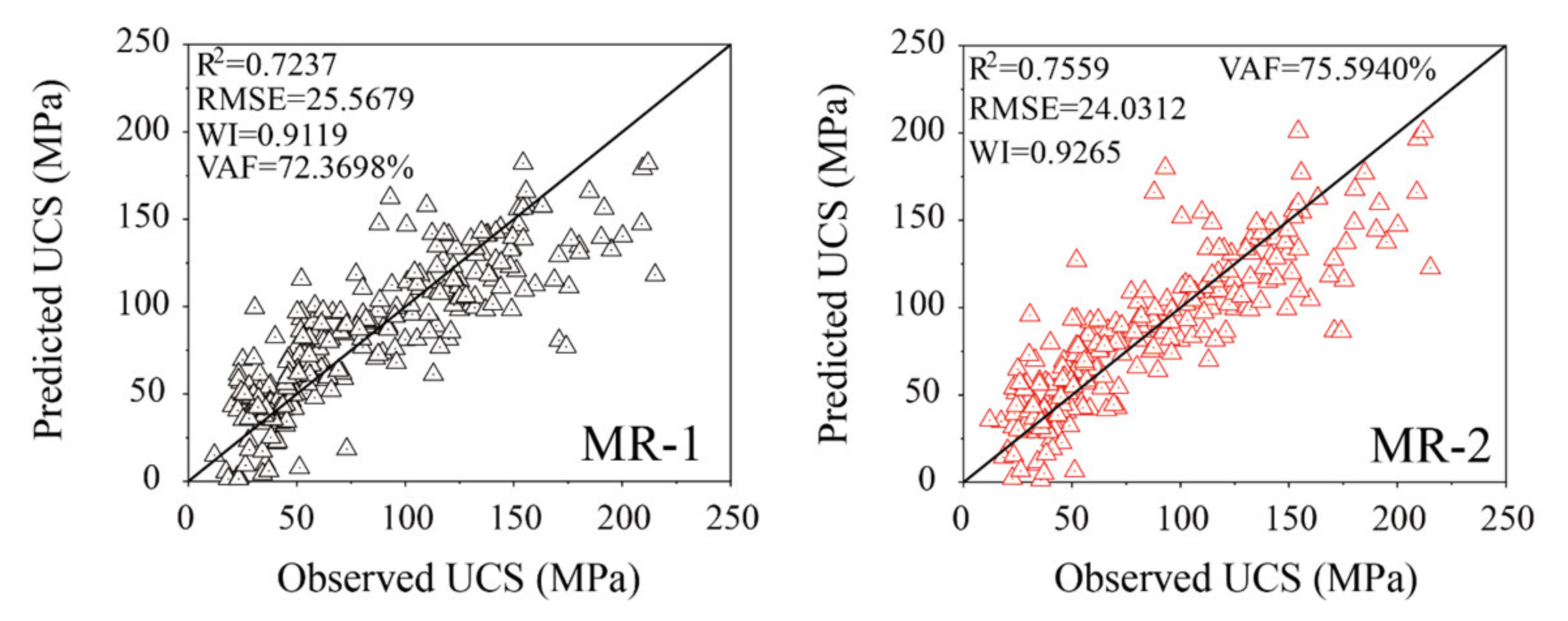
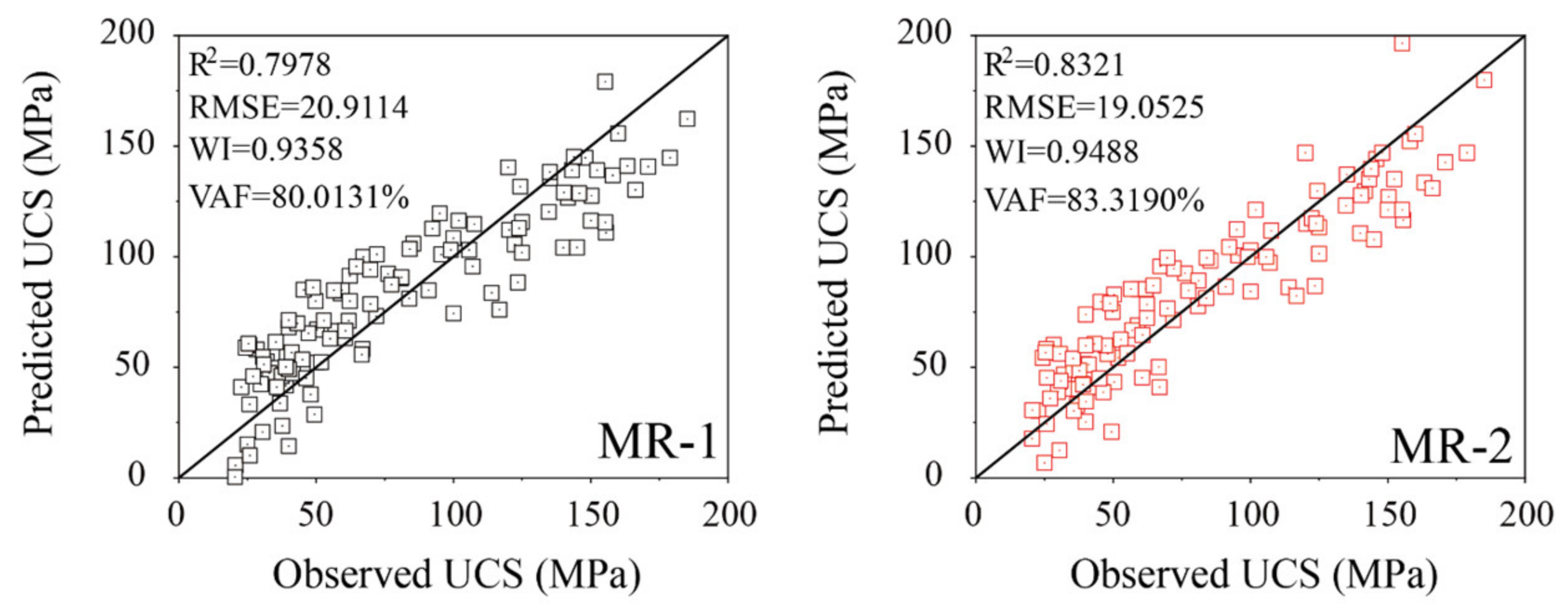
The measured UCS against their predicted values using the multivariate linear and multivariate quadratic MR equations are shown in Figure 3a, b, respectively. As it can be seen in this picture, two MR equations have similar performance in UCS estimation using the almost consistent R². The results of the other three statistical parameters of two MR equations are shown in Table 6.

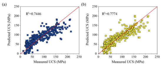
Figure 3. Proposed multiple regression for UCS: (a) Equation (6); (b) Equation (7).

Table 6. Comparison of the performance of all multiple regression models.

Reference	Eqs.	R2	RMSE	WI	VAF (%)
This study	Equation (6)	0.7446	24.2627	0.9187	74.4828
	Equation (7)	0.7774	22.6503	0.9328	77.7455

4.2. AI Methods

To clarify the application of the artificial intelligence methods in the UCS prediction, the RF and one of the four used MHO algorithms called the LSO algorithm are described comprehensively, and the parameter setting and running of the remaining MHO algorithms can be found in the following studies [29,32,65,70,71,72,73].

4.2.1. RF Model

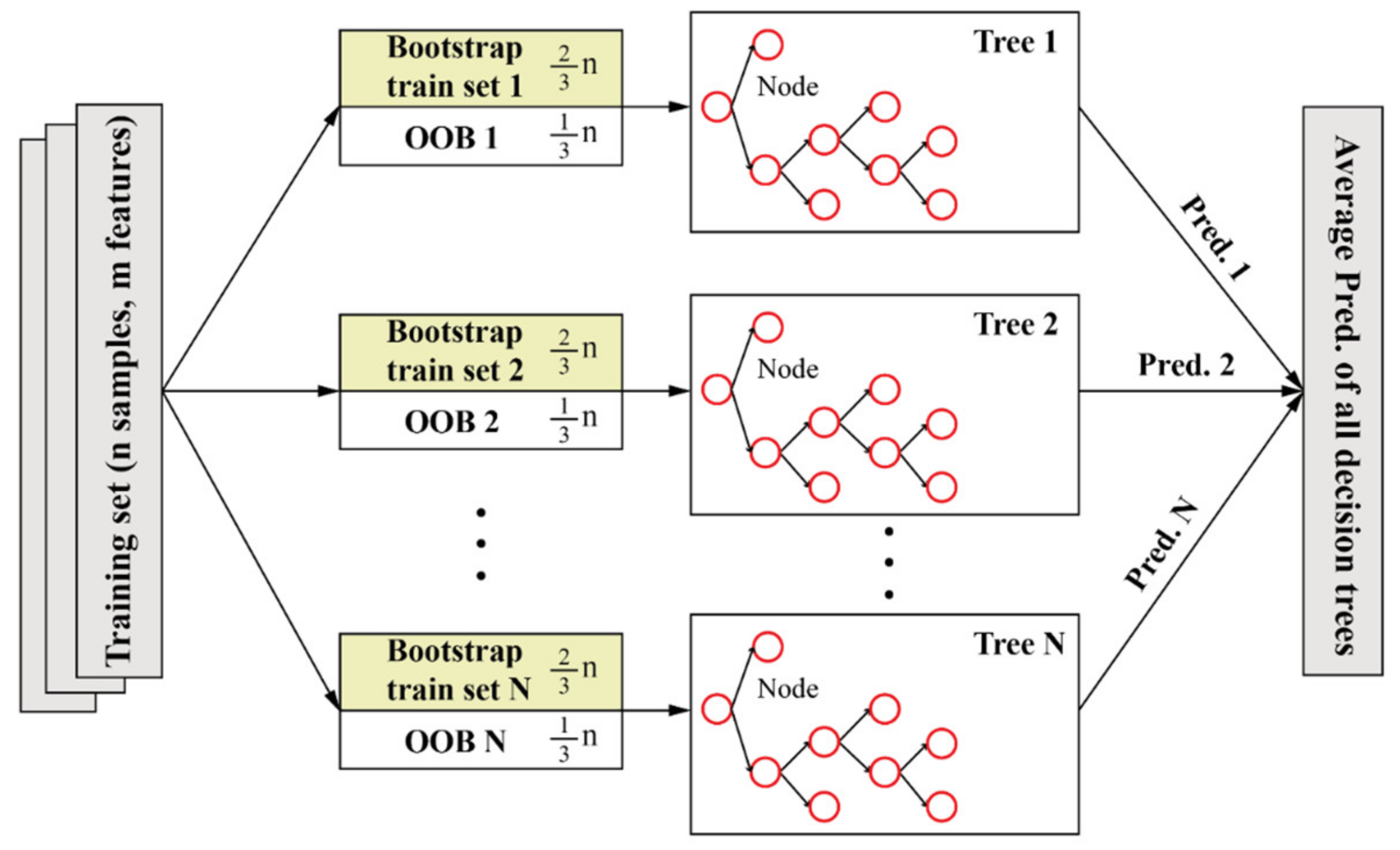
The RF is an ensemble learning method widely used to solve regression and classification problems by means of regression and classification trees (RECT). The development of RF has gone through two phases, i.e., initial random decision forests created by Ho [74] and the extension of the random decision forests improved by Breiman [75]. From a statistical point of view, the resampling is one of the operation criteria of RF model. In other words, each new bootstrap train set is randomly extracted from the original training set to form an independent decision tree model while the unselected samples (one-third of the original training set) form an out-of-bag (OOB) prediction set to be responsible for the prediction performance of each new decision tree. Therefore, the diversity of decision trees can be increased by returning samples and randomly changing the combination of predictors in different tree evolutions. Finally, the prediction results of all decision trees are combined to obtain the average value as the final RF prediction performance. Then, the output of RF model can be described in Equation (8), and the entire process of running a random forest model is shown in Figure 4.

$$R_o=\frac{1}{n}{\displaystyle \sum _{i=1}^n{R}_i(x)},$$

(8)

where $R_o$ represents the average output of RF, $R_i(x)$ denotes the individual output of a tree for on input x, and n represents the total number of decision trees.

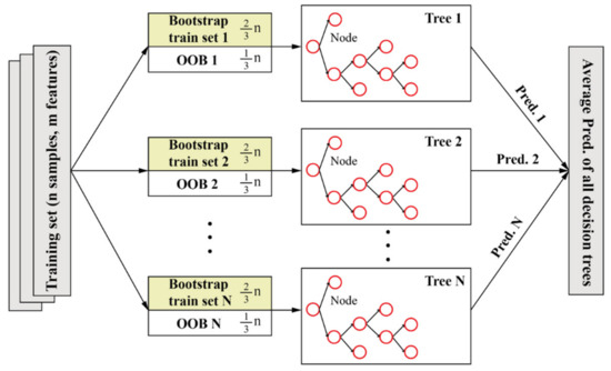
Figure 4. Flowchart of running a random forest.

4.2.2. Hybrid MHO-RF Model Development

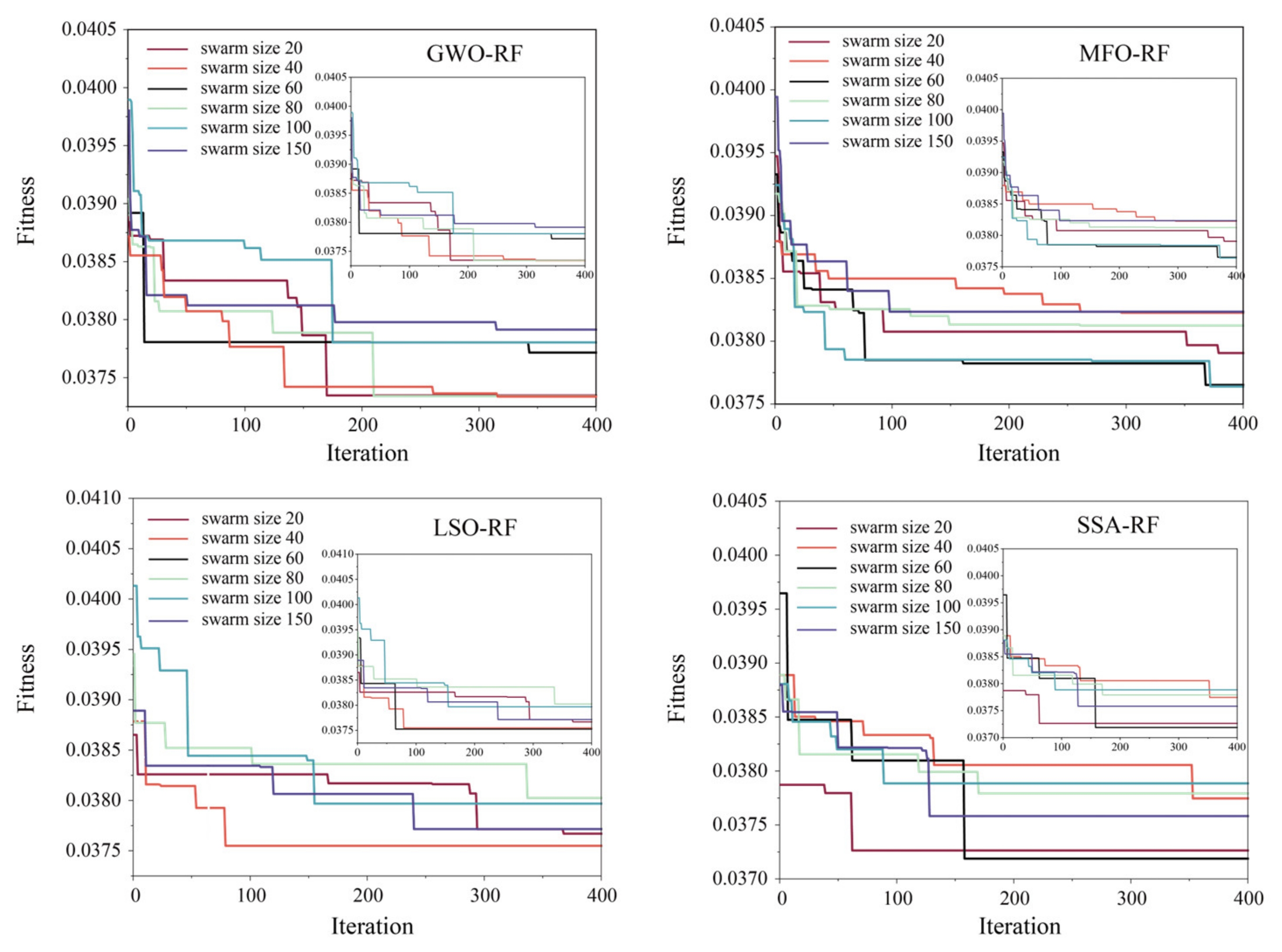
Prior to developing the MHO-RF prediction model, the hyperparametric optimization range of the RF model and the key structural parameters of the four MHO algorithms need to be set in advance. In this study, both the Nt and the Minlefsize are considered in a range of 1–100. For MHO algorithms, the swarm size and iteration are two key impact parameters for tuning hyperparameters [76], which are set as [20, 40, 60, 80, 100, and 150] and 400, respectively. In addition, the train set accounted for 70 percent of the total rock samples, and the remaining 30 percent was used as the test set. All parameters normalized into a pointed range of −1 to 1. To determine the optimal internal parameters of MHO algorithms and the best hyperparameter combination of the RF, the MSE was used to establish the fitness function. Figure 5 shows the effect of the swarm size on the performance of four hybrid models for 400 iterations, respectively. As can be seen in this picture, the best swarm sizes of all MFO models have been obtained by means of the lowest values of the MSE, which are 40 wolves for GWO, 100 moths for MFO, 60 lions for LSO, and 60 sparrows for SSA, respectively.

Figure 5. Optimization MHO-RF models with different swarm sizes for predicting the UCS.

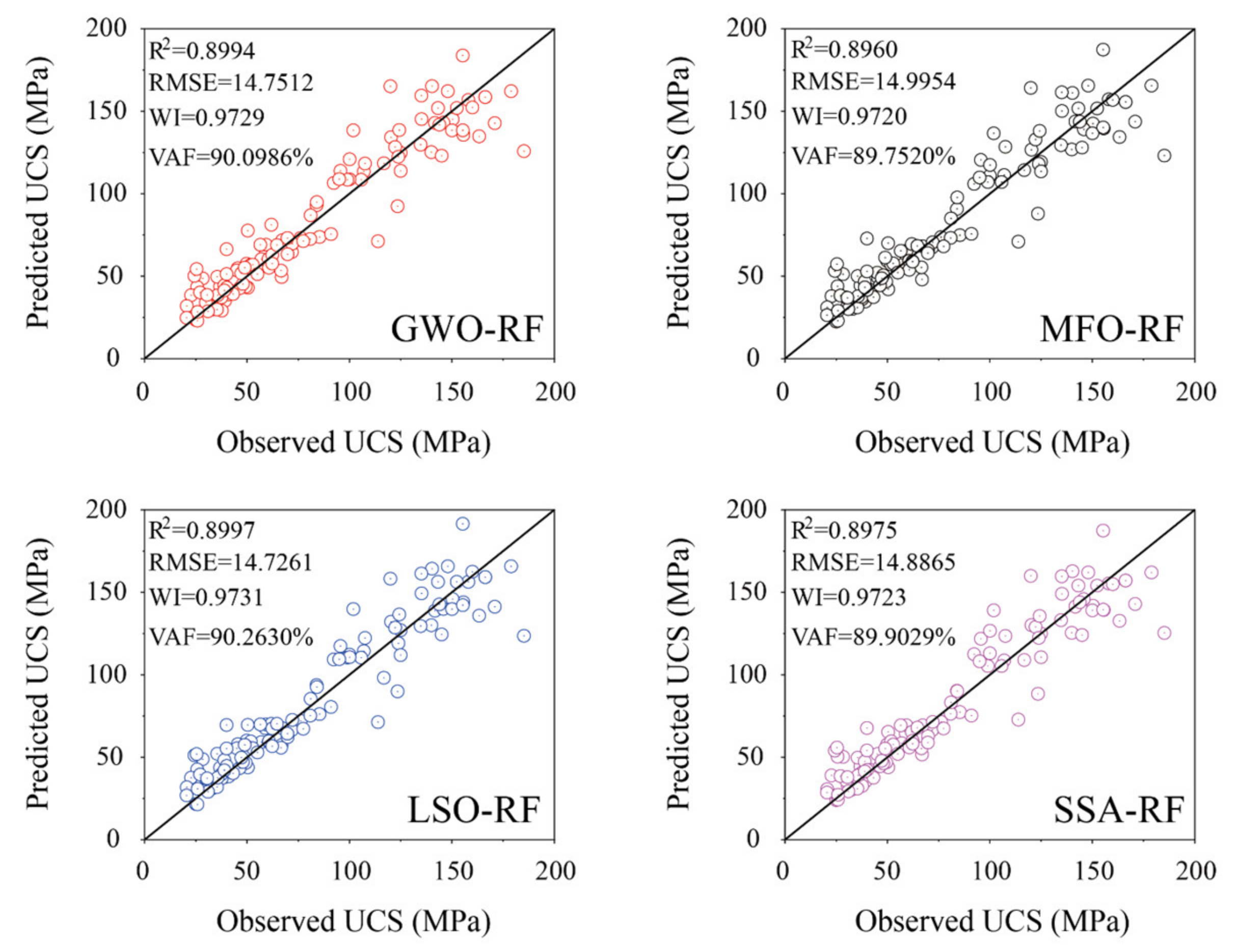
Further comparison results of two performance indices (R² and RMSE) in the training and testing phases for four MHO-RF models are presented in Table 7. As it can be seen in this table, each MHO model with all the considered swarm sizes have been capable of reaching satisfying performance indices in terms of resulting in high values of R² and low values of RMSE in the training phase. Nevertheless, the performance of models with the same swarm size in the testing phase is inconsistent with that in the training phase. As can be realized that the swarm size of 40, 100, 60, and 60 in GWO-RF, MFO-RF, LSO-RF, and SSA-RF with the highest values of R² (0.8994, 0.8960, 0.8997, and 8975) and the lowest values of RMSE (14.7512, 14.9954, 14.7261, and 14.8865) are the best model for the UCS prediction in the testing phase, respectively. Meanwhile, the running time of each model with different swarm sizes has been recorded in this table. The running time is increasing with swarm size, but the time required by the best models is appropriate; thus, these models can be adopted to predict the rock UCS in this study.

Table 7. Comparative performance indicates of MHO-RF model with different swarm sizes.

Model	Swarm Size	R2		RMSE		Time (Sec.)
		Training	Testing	Training	Testing
GWO-RF	20	0.9194	0.8909	13.8053	15.3570	189
	40	0.9188	0.8994	13.8564	14.7512	401
	60	0.9243	0.8854	13.1171	15.7414	575
	80	0.9229	0.8912	13.5070	15.3364	781
	100	0.9250	0.8803	13.3191	16.0884	946
	150	0.9303	0.8762	12.8409	16.3657	1350
Model	Swarm Size	R2		RMSE		Time (Sec.)
		Training	Testing	Training	Testing
MFO-RF	20	0.9219	0.8936	13.5943	15.1714	246
	40	0.9302	0.8867	12.8499	15.6517	375
	60	0.9209	0.8943	13.6767	15.1157	589
	80	0.9213	0.8916	13.6483	15.3081	741
	100	0.9203	0.8960	13.7304	14.9954	1052
	150	0.9297	0.8772	12.9008	16.2968	1489
Model	Swarm Size	R2		RMSE		Time (Sec.)
		Training	Testing	Training	Testing
LSO-RF	20	0.9207	0.8948	13.6983	15.0811	305
	40	0.9175	0.8957	13.9726	15.0169	463
	60	0.9200	0.8997	13.7545	14.7261	687
	80	0.9284	0.8876	13.0185	15.5939	912
	100	0.9208	0.8895	13.6929	15.4621	1150
	150	0.9141	0.8910	14.2522	15.3516	1560
Model	Swarm Size	R2		RMSE		Time (Sec.)
		Training	Testing	Training	Testing
SSA-RF	20	0.9208	0.8927	13.6911	15.2358	315
	40	0.9252	0.8854	13.3036	15.7461	578
	60	0.9224	0.8975	13.5502	14.8865	821
	80	0.9309	0.8837	12.7861	15.8606	1021
	100	0.9279	0.8818	13.0633	15.9858	1468
	150	0.9219	0.8922	13.5977	15.2656	2020

5. Comparison of Prediction Performance

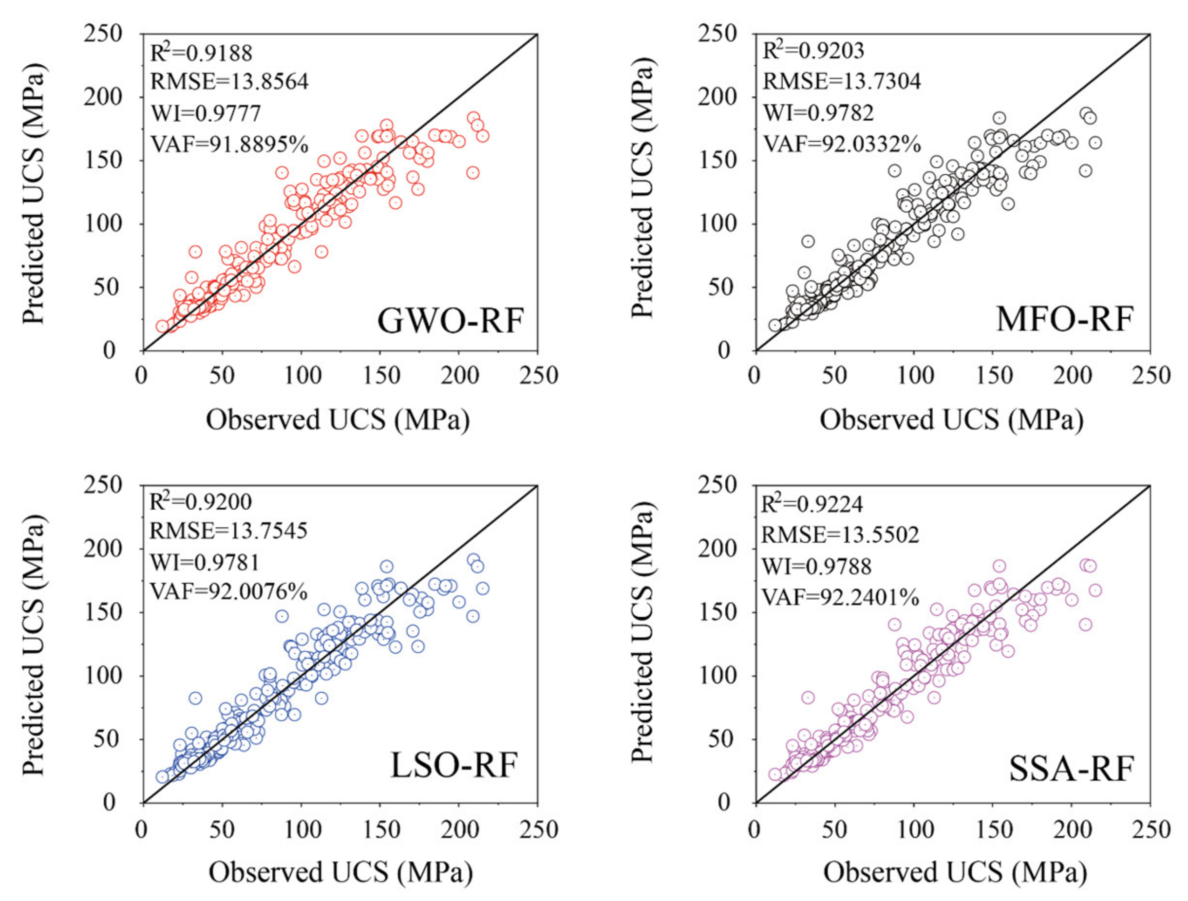
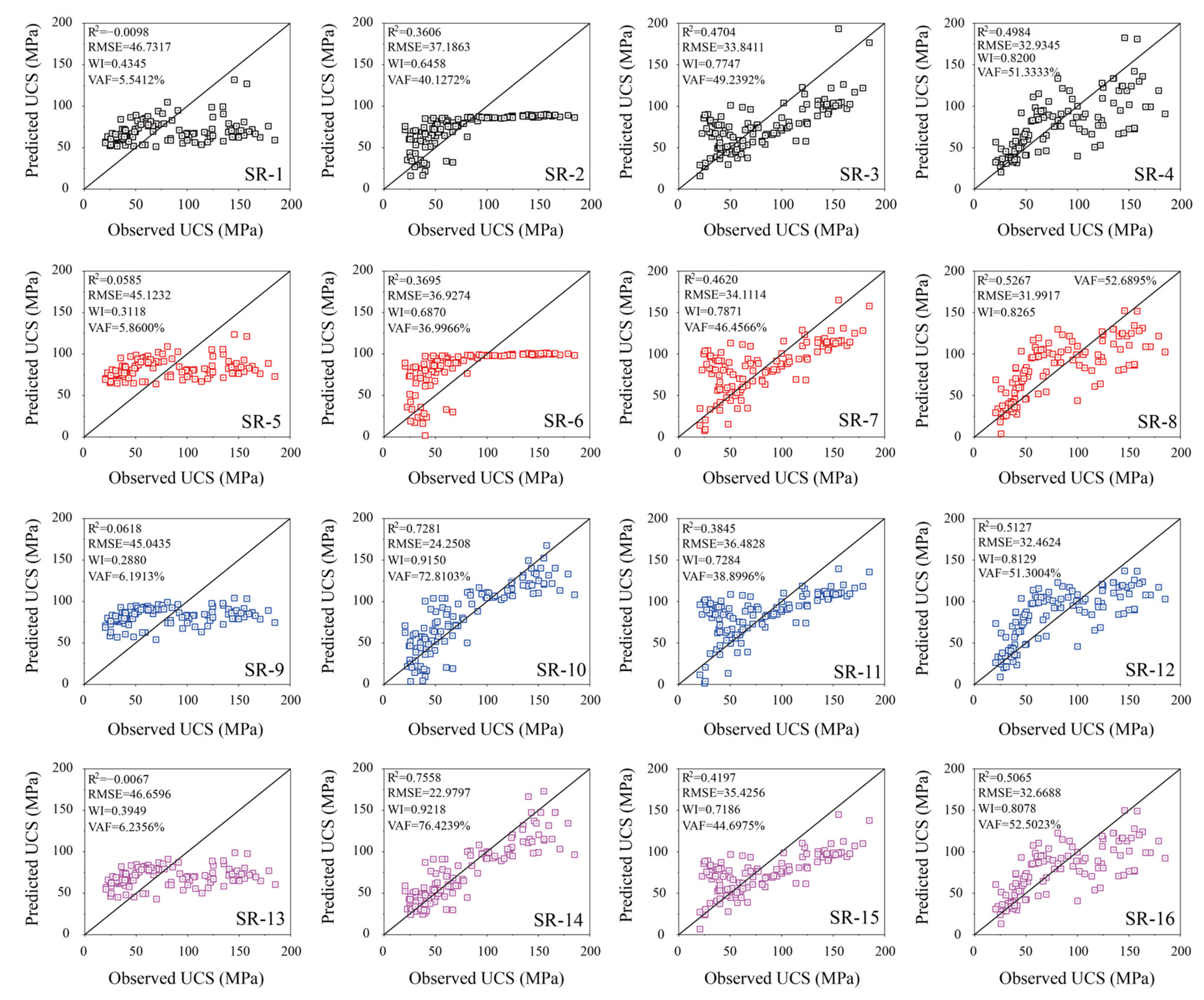
After developing the SR and the MR equations and four MHO-RF methods, a series of comparative evaluation analysis between empirical approaches and AI methods for predicting the rock UCS was conducted in this section. Table 8 illustrates the performance indices results of 16 SR equations, 2 MR equations, and 4 MHO-RF models in the training phase. As can be seen in this table, four SR equations developed by PLS (SR-1. SR-5, SR-9, and SR-13) have poor performance with lower values of R² (even less than zero; this is caused by the very large deviation of the prediction demonstrated in Equation (4)), WI, and VAF and higher values of RMSE. Among these SR equations, SR-14 has obtained the best performance indices of R² = 0.7090, RMSE = 26.2379, WI = 0.8974, and VAF = 71.9010%. By contrast, two MR equations and four hybrid MHO-RF models have satisfactory performance indices by considering high values of R², WI, and VAF (close to 1, 1, and 100%, respectively) and low values of RMSE (close to 0). Among them, the MR-2 (R² = 0.7559, RMSE = 24.0312, WI = 0.9265, and VAF = 75.5940%) and SSA-RF (R² = 0.9224, RMSE = 13.5502, WI = 0.9788, and VAF = 92.2401%.) are the best model of MR equations and all AI models for UCS prediction in the training phase, respectively. However, the prediction performances of the considered four MHO-RF models are obviously superior to two MR equations with higher accuracy.

Table 8. Performance comparison of SR and MR equations and MHO-RF methods in the training phase.

Model	Performance
	R2	RMSE	WI	VAF (%)
SR-1	−0.0135	48.9683	0.4249	5.6413
SR-2	0.3257	39.9415	0.6215	36.3621
SR-3	0.4764	35.1956	0.7901	50.4493
SR-4	0.4386	36.4466	0.7835	45.8063
SR-5	0.0527	47.3417	0.3047	5.2738
SR-6	0.3140	40.2879	0.6754	31.3986
SR-7	0.4903	34.7257	0.8046	49.0569
SR-8	0.4584	35.7952	0.7860	45.8463
SR-9	0.0340	47.8060	0.2633	3.4053
SR-10	0.6441	29.0187	0.8823	64.4087
SR-11	0.4457	36.2127	0.7606	44.5739
SR-12	0.4361	36.5261	0.7696	43.6100
SR-13	−0.032	49.4143	0.3749	4.0102
SR-14	0.7090	26.2379	0.8974	71.9010
SR-15	0.4361	36.5269	0.7369	47.2350
SR-16	0.4405	36.3845	0.7654	46.1874
MR-1	0.7237	25.5679	0.9119	72.3698
MR-2	0.7559	24.0312	0.9265	75.5940
GWO-RF	0.9188	13.8564	0.9777	91.8895
MFO-RF	0.9203	13.7304	0.9782	92.0332
LSO-RF	0.9200	13.7545	0.9781	92.0076
SSA-RF	0.9224	13.5502	0.9788	92.2401

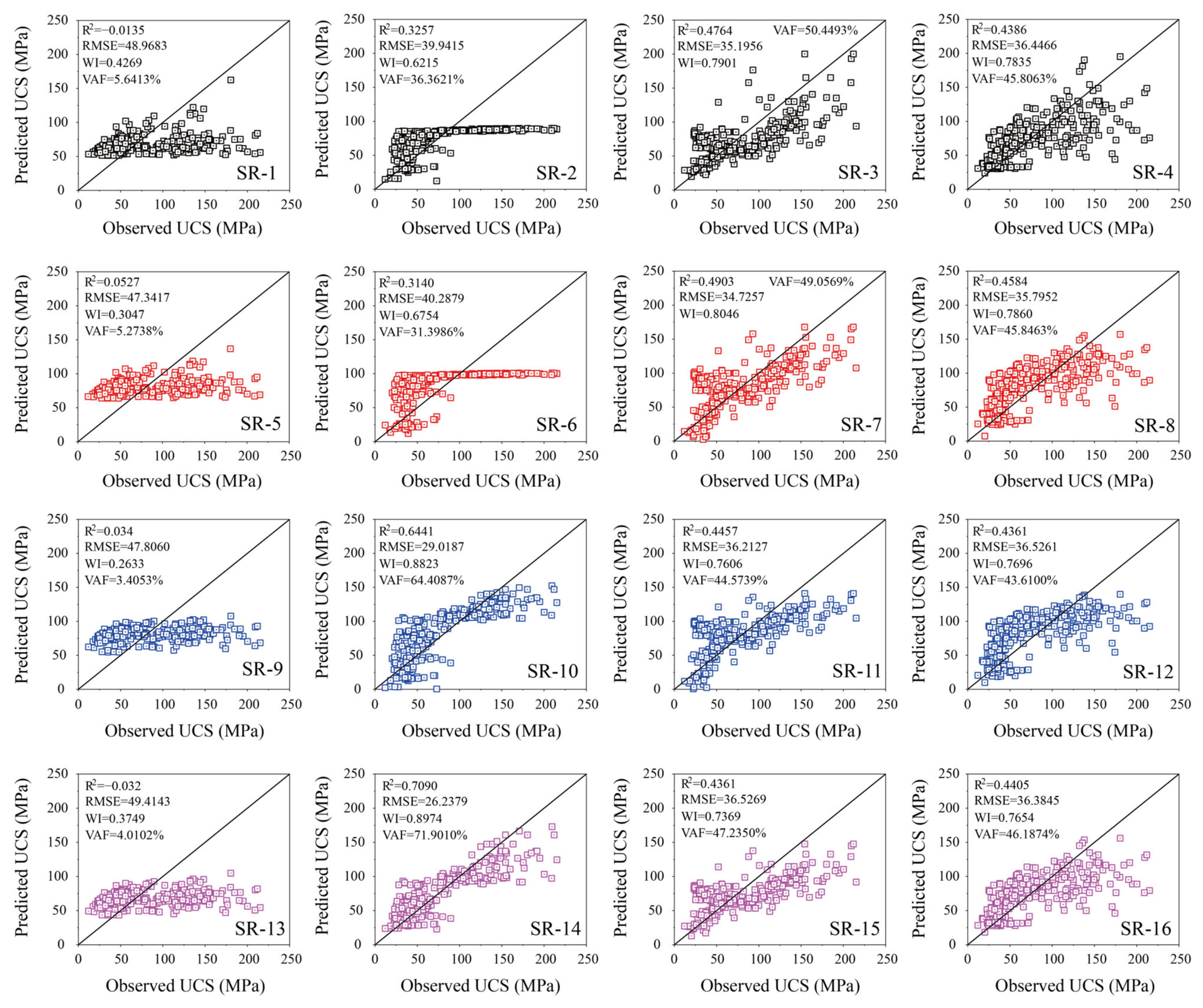
To further compare the performance of empirical approaches and AI models for predicting the UCS, the regression diagrams of all SR and MR equations and four MHO-RF models are demonstrated in Figure 6, Figure 7 and Figure 8. The vertical and horizontal coordinates represent the predicted and observed values of UCS, respectively. The solid black line in each diagram represents the line with 0 error between the predicted and observed UCS. The other dotted lines represent the lines with errors of 10% and 30%, respectively. The significance of these error lines is that the more data points are concentrated on the line with 0 error, the stronger the prediction performance of the model will be. As can be observed in these pictures, the power equation of P_n (SR-14), multivariate quadratic equation (MR-2), and SSA-RF model of MHO models have more data points concentrated on and near the line with 0 error than other models of the same type in the training phase, respectively.

Figure 6. Regression diagrams of the SR models in the training phase.

Figure 7. Regression diagrams of the MR models in the training phase.

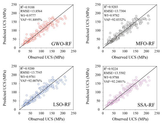
Figure 8. Regression diagrams of the AI models in the training phase.

The performance of the all models in the training phase cannot represent the final performance in the UCS prediction, and it is vital to continue to keep good prediction performance in the testing phase. Table 9 illustrates the performance indices of 16 SR equations, 2 MR equations, and 4 MHO-RF models using the test ser. As it can be seen in this table, the power equation of P_n (SR-14) and MR-2 equation also has a better performance by resulting in higher values of R² (0.7558 and 0.8321), WI (0.9218 and 0.9488) and VAF (76.4239% and 83.3190%), and lower values of RMSE (22.9797 and 19.0525) than other models of the same type, respectively. For AI models, the LSO-RF model has replaced SSA-RF as the best model with the highest accuracy (R² = 0.8997, RMSE = 14.7261, WI = 0.9731, and VAF = 90.2630%) in the testing phase.

Table 9. Performance comparison of the empirical methods and AI models using the test set.

Model	Performance
	R2	RMSE	WI	VAF (%)
SR-1	−0.0098	46.7317	0.4345	5.5412
SR-2	0.3606	37.1863	0.6458	40.1272
SR-3	0.4704	33.8411	0.7747	49.2392
SR-4	0.4984	32.9345	0.8200	51.3333
SR-5	0.0585	45.1232	0.3118	5.8600
SR-6	0.3695	36.9274	0.6870	36.9966
SR-7	0.4620	34.1114	0.7871	46.4566
SR-8	0.5267	31.9917	0.8265	52.6895
SR-9	0.0618	45.0435	0.2880	6.1913
SR-10	0.7281	24.2508	0.9150	72.8103
SR-11	0.3845	36.4828	0.7284	38.8996
SR-12	0.5127	32.4624	0.8129	51.3004
SR-13	−0.0067	46.6596	0.3949	6.2356
SR-14	0.7558	22.9797	0.9218	76.4239
SR-15	0.4197	35.4256	0.7186	44.6975
SR-16	0.5065	32.6688	0.8078	52.5023
MR-1	0.7978	20.9114	0.9358	80.0131
MR-2	0.8321	19.0525	0.9488	83.3190
GWO-RF	0.8994	14.7512	0.9729	90.0986
MFO-RF	0.8960	14.9954	0.9720	89.7520
LSO-RF	0.8997	14.7261	0.9731	90.2630
SSA-RF	0.8975	14.8865	0.9723	89.9029

The necessary validation can prevent the adverse result of the inconsistent performance of the aforementioned models in the training and testing phase. Figure 9, Figure 10 and Figure 11 show the regression diagrams of all SR and MR equations and four MHO-RF models in the testing phase. As it can be seen in these pictures, the SSA-RF obtained an unsatisfactory prediction performance compared to the training phase in terms of resulting in fewer data points clustered on the line with 0 error. Conversely, the LSO-RF model has the largest number of concentrated points on the line with 0 error, and the power equation of P_n (SR-14) and multivariate quadratic equation (MR-2) also have more data points concentrated on and near the line with 0 error than other models of the same type in the testing phase, respectively.

Figure 9. Regression diagrams of the SR models in the testing phase.

Figure 10. Regression diagrams of the MR models in the testing phase.

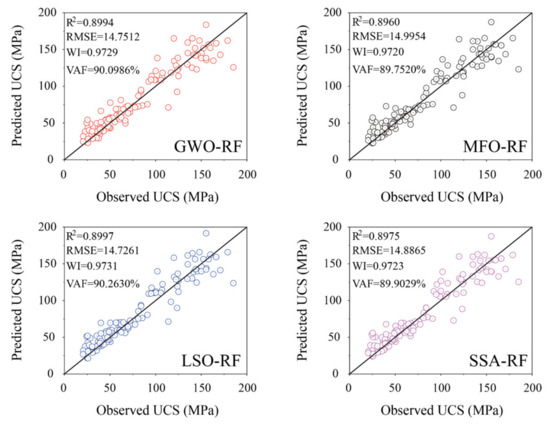
Figure 11. Regression diagrams of the AI models in the testing phase.

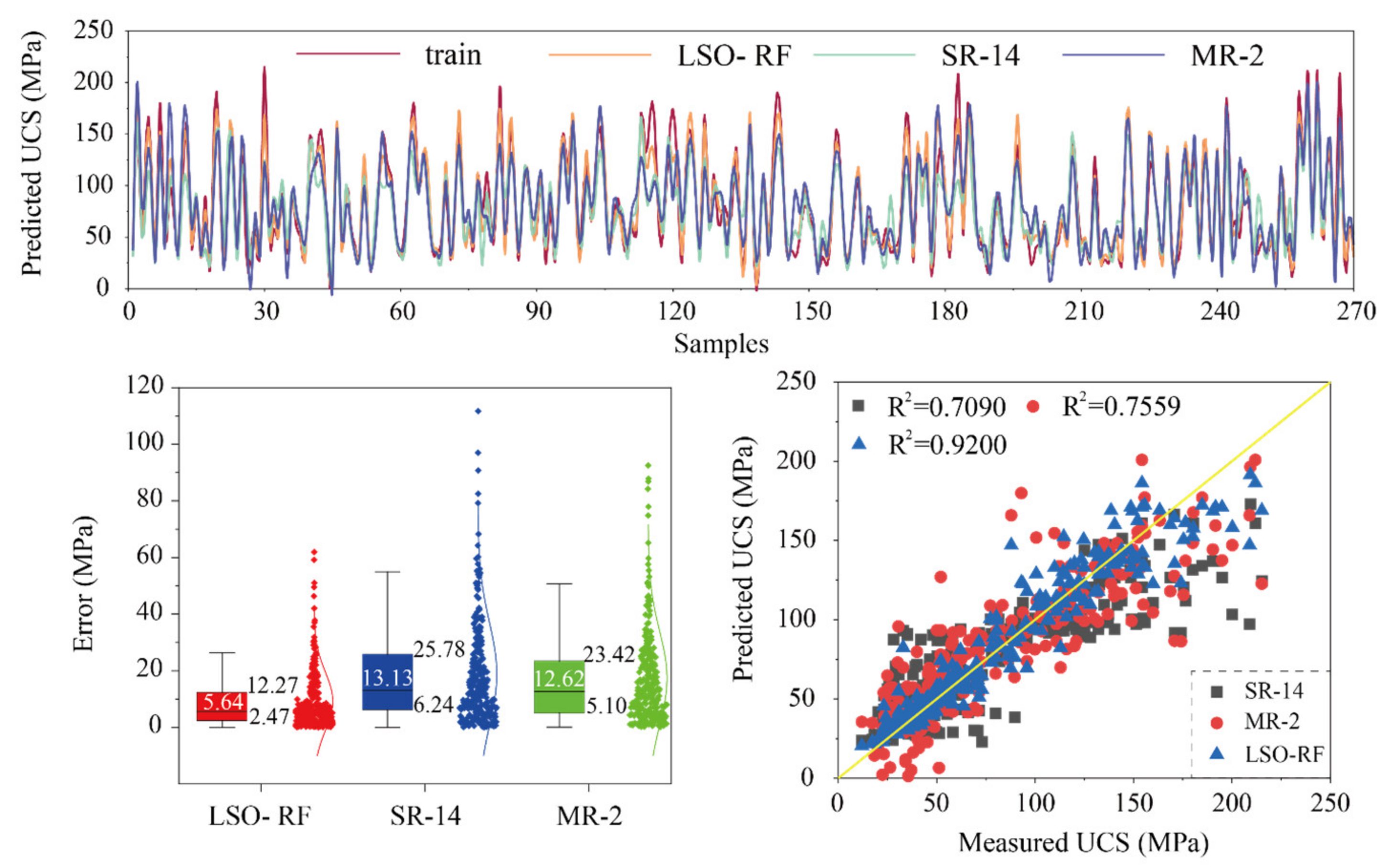
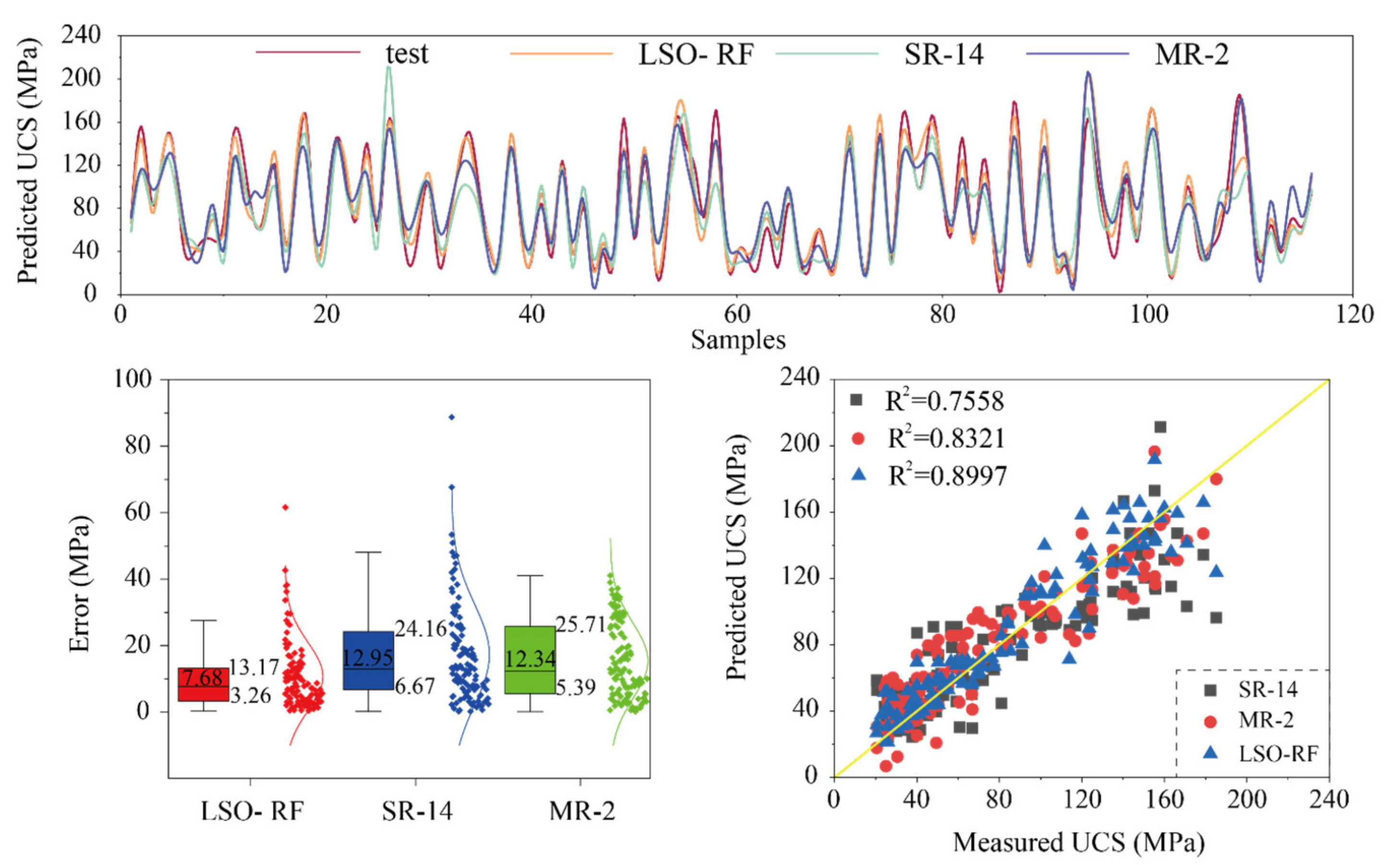
Based on the performance results in Table 8 and Table 9, the best model based on the empirical approaches and AI models is the SR equation of P_n, the MR equation of multivariate quadratic, and the LSO-RF model, respectively. To clearly compare the performance differences between empirical models and AI methods in predicting UCS, the graphs include compressive curves, error analyses, and the regression diagrams of the UCS predicted by empirical and artificial intelligence models in the training phase, which are shown in Figure 12. As it can be seen in Figure 12a, the prediction curves of UCS for the three models are basically consistent with the original training curve, but the LSO-RF model has obviously better performance. The distribution of errors between the observed and predicted UCS of the three models is shown in Figure 12b. The LSO-RF model has the lowest median value of error (5.64), and the SR equation of n has the largest median value of error (13.13). Meanwhile, the upper and lower errors obtained by the SR model are broader than the other two models, which represent the worse prediction performance. Figure 12c shows the regression diagram of all models in the training phase. As it can be observed in this diagram, the LSO-RF model not only has more data points clustered on the line with 0 error, but it also has the highest value of R² (0.9200). After this model, the MR equation of multivariate quadratic has a better prediction performance than the SR equation of P_n. The same results of performance comparison have been obtained in the testing phase, as shown in Figure 13.

Figure 12. Compressive UCS prediction in the training phase.

Figure 13. Compressive UCS prediction in the testing phase.

To further accurately evaluate the performance of all models in the testing phase, the graphical Taylor diagram is also drawn in Figure 14. A typical Taylor diagram can be divided into three parts, i.e., correlation coefficient, standard deviation, and RMSE. As it can be seen in this picture, the red arcs and dots represent the correlation coefficient, the black arcs and dots represent standard deviation, and the green arcs and dots represent RMSE. The RMSE and correlation coefficient of the test data is defaulted to 0 and 1, respectively. Then, the prediction performance is determined by a correlation coefficient, standard deviation, and RMSE, which will be compared with those of the measured data in the test set. It can be observed that the LSO-RF is the best model with the closest position to the test.

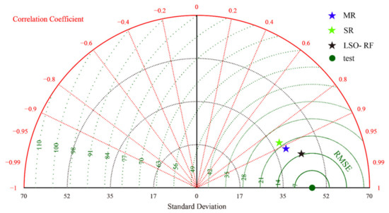
Figure 14. Taylor diagram for comparison of the empirical and artificial intelligence models.

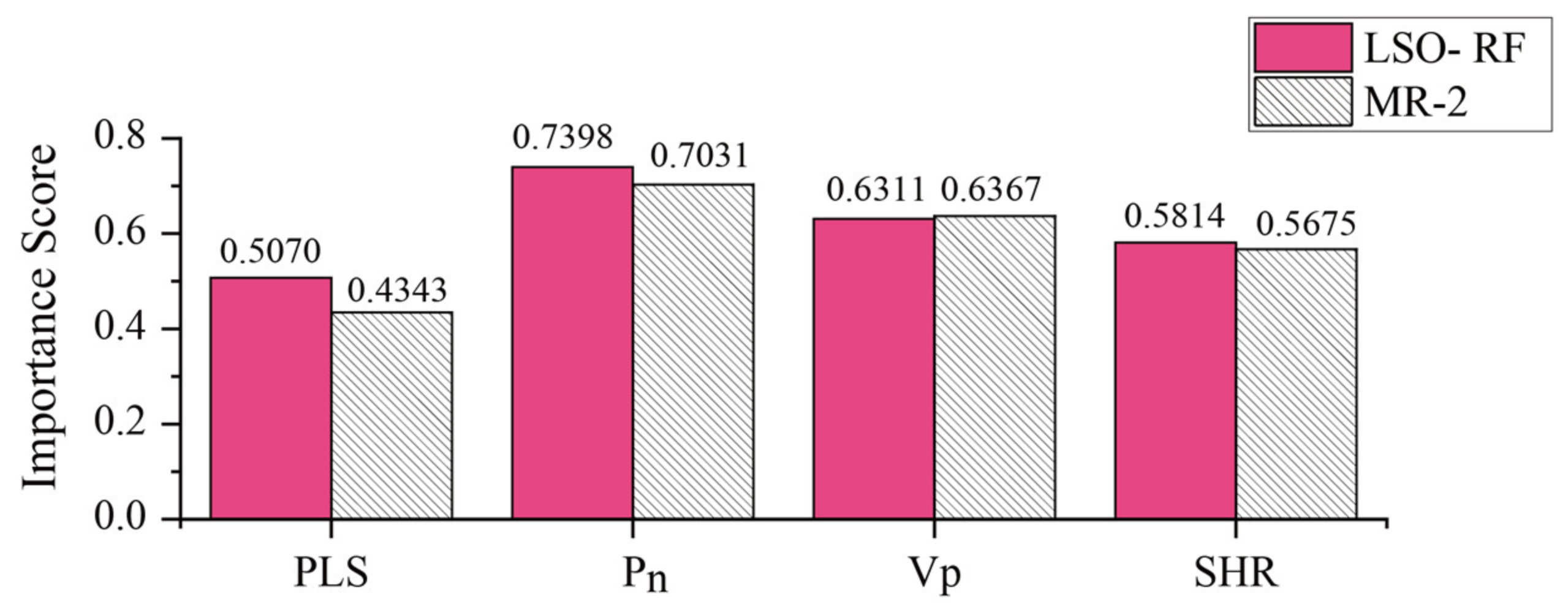
After determining the best model for predicting the UCS of rock, the importance of input variables can be estimated by using the LSO-RF model. In addition, the MR equation of multivariate quadratic is also used to calculate the importance of input variables for comparison with the LSO-RF model. The results of the sensitivity analysis are shown in Figure 15. As it can be seen in this picture, the most important input variable is the P_n with the scores of 0.7398 and 0.7031 obtained from the LSO-RF model and MR equation, respectively. The order of importance of the remaining parameters is the V_p (LSO-RF: 0.6311 and MR: 0.6367), the SHR (LSO-RF: 0.5814 and MR: 0.5675), and the PLS (LSO-RF: 0.5070 and MR: 0.4343).

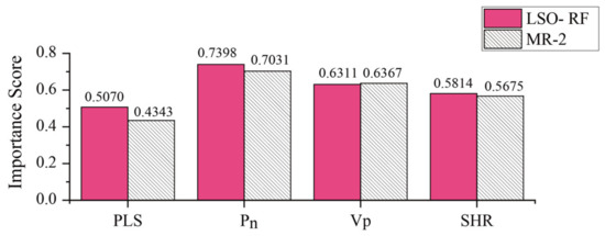
Figure 15. Importance of input variables based on empirical and AI models.

6. Conclusions and Summary

As one of the most important physical and mechanical characteristic parameters for rocks in civil and mining engineering, the UCS can be estimated using various methods. In this study, the widely used empirical approaches by mining engineers and recently concerning AI methods were developed and compared in UCS predicting. A total of 386 rock samples were collected to form a dataset, and the P_n, the SHR, the V_p, and the PLS are considered input variables. The results of performance indices showed that the power equation of P_n and multivariate quadratic equation are the best models of SR and MR equations, respectively, and all MHO-RF models of AI techniques have superior performance than empirical approaches for predicting the rock UCS. However, the LSO-RF model is the best model among the three AI excellent models by means of higher R² (0.9200; 0.8997), WI (0.9781 and 0.9731), and VAF (92.0076%; 90.2630%) and lower values of RMSE (13.7545; 14.7261) in the training and testing phases, respectively. Meanwhile, the sensitive analysis results illustrated that the P_n is the most important input variable for predicting the rock UCS.

Compared with the empirical method to predict the rock UCS, the advantages of AI techniques are strong data compatibility and model generalization. Since only nine rock types from three major lithologies were collected to train the AI models, the prediction accuracy for other rock types other than that used in this paper is not guaranteed. Therefore, more UCS data from various rock types should be supplemented to further improve the prediction accuracy of the proposed models. However, the random population initialization tends to trap optimization into local minima. Therefore, the LSO algorithm must be further optimized to select the optimal model hyperparameters. The chaos mapping can be introduced to achieve this goal. Furthermore, other AI models should also be developed to predict the UCS for generating a multivariate mixing model to adapt to UCS estimations of different rocks.

References

- Aladejare, A.E. Evaluation of empirical estimation of uniaxial compressive strength of rock using measurements from index and physical tests. J. Rock Mech. Geotech. Eng. 2020, 12, 256–268. [Google Scholar] [CrossRef]
- Aladejare, A.E.; Wang, Y. Estimation of rock mass deformation modulus using indirect information from multiple sources. Tunn. Undergr. Space Technol. 2019, 85, 76–83. [Google Scholar] [CrossRef]
- Mahmoodzadeh, A.; Mohammadi, M.; Ibrahim, H.H.; Abdulhamid, S.N.; Salim, S.G.; Ali, H.F.H.; Majeed, M.K. Artificial intelligence forecasting models of uniaxial compressive strength. Transp. Geotech. 2021, 27, 100499. [Google Scholar] [CrossRef]
- Gunsallus, K.T.; Kulhawy, F.H. A comparative evaluation of rock strength measures. Int. J. Rock Mech. Min. Sci. Geomech. Abstr. 1984, 21, 233–248. [Google Scholar] [CrossRef]
- Tuğrul, A.; Zarif, I.H. Correlation of mineralogical and textural characteristics with engineering properties of selected granitic rocks from Turkey. Eng. Geol. 1999, 51, 303–317. [Google Scholar] [CrossRef]
- Gokceoglu, C.; Zorlu, K. A fuzzy model to predict the uniaxial compressive strength and the modulus of elasticity of a problematic rock. Eng. Appl. Artif. Intell. 2004, 17, 61–72. [Google Scholar] [CrossRef]
- Kahraman, S.; Gunaydin, O. The effect of rock classes on the relation between uniaxial compressive strength and point load index. Bull. Eng. Geol. Environ. 2009, 68, 345–353. [Google Scholar] [CrossRef]
- Dehghan, S.; Sattari, G.H.; Chelgani, S.C.; Aliabadi, M.A. Prediction of uniaxial compressive strength and modulus of elasticity for Travertine samples using regression and artificial neural networks. Min. Sci. Technol. 2010, 20, 41–46. [Google Scholar] [CrossRef]
- Armaghani, D.J.; Tonnizam Mohamad, E.; Momeni, E.; Monjezi, M.; Sundaram Narayanasamy, M. Prediction of the strength and elasticity modulus of granite through an expert artificial neural network. Arab. J. Geosci. 2016, 9, 48. [Google Scholar] [CrossRef]
- Armaghani, D.J.; Tonnizam Mohamad, E.; Hajihassani, M.; Yagiz, S.; Motaghedi, H. Application of several non-linear prediction tools for estimating uniaxial compressive strength of granitic rocks and comparison of their performances. Eng. Comput. 2016, 32, 189–206. [Google Scholar] [CrossRef]
- Aliyu, M.M.; Shang, J.; Murphy, W.; Lawrence, J.A.; Collier, R.; Kong, F.; Zhao, Z. Assessing the uniaxial compressive strength of extremely hard cryptocrystalline flint. Int. J. Rock Mech. Min. Sci. 2019, 113, 310–321. [Google Scholar] [CrossRef]
- Momeni, E.; Armaghani, D.J.; Hajihassani, M.; Amin, M.F.M. Prediction of uniaxial compressive strength of rock samples using hybrid particle swarm optimization-based artificial neural networks. Measurement 2015, 60, 50–63. [Google Scholar] [CrossRef]
- Heidari, M.; Mohseni, H.; Jalali, S.H. Prediction of uniaxial compressive strength of some sedimentary rocks by fuzzy and regression models. Geotech. Geol. Eng. 2018, 36, 401–412. [Google Scholar] [CrossRef]
- Wang, Y.; Aladejare, A.E. Bayesian characterization of correlation between uniaxial compressive strength and Young’s modulus of rock. Int. J. Rock Mech. Min. Sci. 2016, 85, 10–19. [Google Scholar] [CrossRef]
- Aladejare, A.E.; Alofe, E.D.; Onifade, M.; Lawal, A.I.; Ozoji, T.M.; Zhang, Z.X. Empirical estimation of uniaxial compressive strength of rock: Database of simple, multiple, and artificial intelligence-based regressions. Geotech. Geol. Eng. 2021, 39, 4427–4455. [Google Scholar] [CrossRef]
- Rabbani, E.; Sharif, F.; Salooki, M.K.; Moradzadeh, A. Application of neural network technique for prediction of uniaxial compressive strength using reservoir formation properties. Int. J. Rock Mech. Min. Sci. 2012, 56, 100–111. [Google Scholar] [CrossRef]
- Torabi-Kaveh, M.; Naseri, F.; Saneie, S.; Sarshari, B. Application of artificial neural networks and multivariate statistics to predict UCS and E using physical properties of Asmari limestones. Arab. J. Geosci. 2015, 8, 2889–2897. [Google Scholar] [CrossRef]
- Madhubabu, N.; Singh, P.K.; Kainthola, A.; Mahanta, B.; Tripathy, A.; Singh, T.N. Prediction of compressive strength and elastic modulus of carbonate rocks. Measurement 2016, 88, 202–213. [Google Scholar] [CrossRef]
- Yilmaz, I.; Yuksek, G. Prediction of the strength and elasticity modulus of gypsum using multiple regression, ANN, and ANFIS models. Int. J. Rock Mech. Min. Sci. 2009, 46, 803–810. [Google Scholar] [CrossRef]
- Barzegar, R.; Sattarpour, M.; Nikudel, M.R.; Moghaddam, A.A. Comparative evaluation of artificial intelligence models for prediction of uniaxial compressive strength of travertine rocks, case study: Azarshahr area, NW Iran. Model. Earth Syst. Environ. 2016, 2, 76. [Google Scholar] [CrossRef]
- Ceryan, N. Application of support vector machines and relevance vector machines in predicting uniaxial compressive strength of volcanic rocks. J. Afr. Earth Sci. 2014, 100, 634–644. [Google Scholar] [CrossRef]
- Çelik, S.B. Prediction of uniaxial compressive strength of carbonate rocks from nondestructive tests using multivariate regression and LS-SVM methods. Arab. J. Geosci. 2019, 12, 193–210. [Google Scholar] [CrossRef]
- Asheghi, R.; Abbaszadeh Shahri, A.; Khorsand Zak, M. Prediction of uniaxial compressive strength of different quarried rocks using metaheuristic algorithm. Arab. J. Sci. Eng. 2019, 44, 8645–8659. [Google Scholar] [CrossRef]
- Matin, S.S.; Farahzadi, L.; Makaremi, S.; Chelgani, S.C.; Sattari, G.H. Variable selection and prediction of uniaxial compressive strength and modulus of elasticity by random forest. Appl. Soft Comput. 2018, 70, 980–987. [Google Scholar] [CrossRef]
- Dai, Y.; Khandelwal, M.; Qiu, Y.; Zhou, J.; Monjezi, M.; Yang, P. A hybrid metaheuristic approach using random forest and particle swarm optimization to study and evaluate backbreak in open-pit blasting. Neural Comput. Appl. 2022, 34, 6273–6288. [Google Scholar] [CrossRef]
- Mohamad, E.T.; Jahed Armaghani, D.; Momeni, E.; Alavi Nezhad Khalil Abad, S.V. Prediction of the unconfined compressive strength of soft rocks: A PSO-based ANN approach. Bull. Eng. Geol. Environ. 2015, 74, 745–757. [Google Scholar] [CrossRef]
- Sun, Y.; Li, G.; Zhang, N.; Chang, Q.; Xu, J.; Zhang, J. Development of ensemble learning models to evaluate the strength of coal-grout materials. Int. J. Min. Sci. Technol. 2021, 31, 153–162. [Google Scholar] [CrossRef]
- Xu, C.; Nait Amar, M.; Ghriga, M.A.; Ouaer, H.; Zhang, X.; Hasanipanah, M. Evolving support vector regression using Grey Wolf optimization; forecasting the geomechanical properties of rock. Eng. Comput. 2022, 38, 1819–1833. [Google Scholar] [CrossRef]
- Zhou, J.; Huang, S.; Zhou, T.; Armaghani, D.J.; Qiu, Y. Employing a genetic algorithm and grey wolf optimizer for optimizing RF models to evaluate soil liquefaction potential. Artif. Intell. Rev. 2022, 55, 5673–5705. [Google Scholar] [CrossRef]
- Fattahi, H. Applying soft computing methods to predict the uniaxial compressive strength of rocks from schmidt hammer rebound values. Comput. Geosci. 2017, 21, 665–681. [Google Scholar] [CrossRef]
- Zhang, J.; Li, D.; Wang, Y. Toward intelligent construction: Prediction of mechanical properties of manufactured-sand concrete using tree-based models. J. Clean. Prod. 2020, 258, 120665. [Google Scholar] [CrossRef]
- Zhou, J.; Huang, S.; Qiu, Y. Optimization of random forest through the use of MVO, GWO and MFO in evaluating the stability of underground entry-type excavations. Tunn. Undergr. Space Technol. 2022, 124, 104494. [Google Scholar] [CrossRef]
- Yu, Z.; Shi, X.; Qiu, X.; Zhou, J.; Chen, X.; Gou, Y. Optimization of postblast ore boundary determination using a novel sine cosine algorithm-based random forest technique and Monte Carlo simulation. Eng. Optim. 2021, 53, 1467–1482. [Google Scholar] [CrossRef]
- Ghasemi, E.; Kalhori, H.; Bagherpour, R.; Yagiz, S. Model tree approach for predicting uniaxial compressive strength and Young’s modulus of carbonate rocks. Bull. Eng. Geol. Environ. 2018, 77, 331–343. [Google Scholar] [CrossRef]
- Basu, A.; Kamran, M. Point load test on schistose rocks and its applicability in predicting uniaxial compressive strength. Int. J. Rock Mech. Min. Sci. 2010, 47, 823–828. [Google Scholar] [CrossRef]
- Mishra, D.A.; Basu, A. Use of the block punch test to predict the compressive and tensile strengths of rocks. Int. J. Rock Mech. Min. Sci. 2012, 51, 119–127. [Google Scholar] [CrossRef]
- Xie, S.; Lin, H.; Duan, H.; Chen, Y. Modeling description of interface shear deformation: A theoretical study on damage statistical distributions. Constr. Build. Mater. 2023, 394, 132052. [Google Scholar] [CrossRef]
- Gupta, V. Non-destructive testing of some Higher Himalayan Rocks in the Satluj Valley. Bull. Eng. Geol. Environ. 2009, 68, 409–416. [Google Scholar] [CrossRef]
- Tsiambaos, G.; Sabatakakis, N. Considerations on strength of intact sedimentary rocks. Eng. Geol. 2004, 72, 261–273. [Google Scholar] [CrossRef]
- Kohno, M.; Maeda, H. Relationship between point load strength index and uniaxial compressive strength of hydrothermally altered soft rocks. Int. J. Rock Mech. Min. Sci. 2012, 50, 147–157. [Google Scholar] [CrossRef]
- Palchik, V.; Hatzor, Y.H. The influence of porosity on tensile and compressive strength of porous chalks. Rock Mech. Rock Eng. 2004, 37, 331–341. [Google Scholar] [CrossRef]
- Diamantis, K.; Gartzos, E.; Migiros, G. Study on uniaxial compressive strength, point load strength index, dynamic and physical properties of serpentinites from Central Greece: Test results and empirical relations. Eng. Geol. 2009, 108, 199–207. [Google Scholar] [CrossRef]
- Mishra, D.A.; Basu, A. Estimation of uniaxial compressive strength of rock materials by index tests using regression analysis and fuzzy inference system. Eng. Geol. 2013, 160, 54–68. [Google Scholar] [CrossRef]
- Entwisle, D.C.; Hobbs, P.R.N.; Jones, L.D.; Gunn, D.; Raines, M.G. The relationships between effective porosity, uniaxial compressive strength and sonic velocity of intact Borrowdale Volcanic Group core samples from Sellafield. Geotech. Geol. Eng. 2005, 23, 793–809. [Google Scholar] [CrossRef]
- Beiki, M.; Majdi, A.; Givshad, A.D. Application of genetic programming to predict the uniaxial compressive strength and elastic modulus of carbonate rocks. Int. J. Rock Mech. Min. Sci. 2013, 63, 159–169. [Google Scholar] [CrossRef]
- Aydin, A.; Basu, A. The Schmidt hammer in rock material characterization. Eng. Geol. 2005, 81, 1–14. [Google Scholar] [CrossRef]
- Kılıç, A.; Teymen, A. Determination of mechanical properties of rocks using simple methods. Bull. Eng. Geol. Environ. 2008, 67, 237–244. [Google Scholar] [CrossRef]
- Çobanoğlu, İ.; Çelik, S.B. Estimation of uniaxial compressive strength from point load strength, Schmidt hardness and P-wave velocity. Bull. Eng. Geol. Environ. 2008, 67, 491–498. [Google Scholar] [CrossRef]
- Ali, E.; Guang, W.; Ibrahim, A. Empirical relations between compressive strength and microfabric properties of amphibolites using multivariate regression, fuzzy inference and neural networks: A comparative study. Eng. Geol. 2014, 183, 230–240. [Google Scholar] [CrossRef]
- Cheshomi, A.; Mousavi, E.; Ahmadi-Sheshde, E. Evaluation of single particle loading test to estimate the uniaxial compressive strength of sandstone. J. Pet. Sci. Eng. 2015, 135, 421–428. [Google Scholar] [CrossRef]
- Selçuk, L.; Kayabali, K. Evaluation of the unconfined compressive strength of rocks using nail guns. Eng. Geol. 2015, 195, 164–171. [Google Scholar] [CrossRef]
- Uyanık, O.; Sabbağ, N.; Uyanık, N.A.; Öncü, Z. Prediction of mechanical and physical properties of some sedimentary rocks from ultrasonic velocities. Bull. Eng. Geol. Environ. 2019, 78, 6003–6016. [Google Scholar] [CrossRef]
- Karakus, M.; Tutmez, B. Fuzzy and multiple regression modelling for evaluation of intact rock strength based on point load, Schmidt hammer and sonic velocity. Rock Mech. Rock Eng. 2006, 39, 45–57. [Google Scholar] [CrossRef]
- Ng, I.T.; Yuen, K.V.; Lau, C.H. Predictive model for uniaxial compressive strength for Grade III granitic rocks from Macao. Eng. Geol. 2015, 199, 28–37. [Google Scholar] [CrossRef]
- Jalali, S.H.; Heidari, M.; Mohseni, H. Comparison of models for estimating uniaxial compressive strength of some sedimentary rocks from Qom Formation. Environ. Earth Sci. 2017, 76, 1–15. [Google Scholar] [CrossRef]
- Sharma, L.K.; Vishal, V.; Singh, T.N. Developing novel models using neural networks and fuzzy systems for the prediction of strength of rocks from key geomechanical properties. Measurement 2017, 102, 158–169. [Google Scholar] [CrossRef]
- Aboutaleb, S.; Behnia, M.; Bagherpour, R.; Bluekian, B. Using non-destructive tests for estimating uniaxial compressive strength and static Young’s modulus of carbonate rocks via some modeling techniques. Bull. Eng. Geol. Environ. 2018, 77, 1717–1728. [Google Scholar] [CrossRef]
- Zhou, J.; Huang, S.; Wang, M.; Qiu, Y. Performance evaluation of hybrid GA–SVM and GWO–SVM models to predict earthquake-induced liquefaction potential of soil: A multi-dataset investigation. Eng. Comput. 2021, 38, 4197–4215. [Google Scholar] [CrossRef]
- Zhou, J.; Qiu, Y.; Zhu, S.; Armaghani, D.J.; Li, C.; Nguyen, H.; Yagiz, S. Optimization of support vector machine through the use of metaheuristic algorithms in forecasting TBM advance rate. Eng. Appl. Artif. Intell. 2021, 97, 104015. [Google Scholar] [CrossRef]
- Zhou, J.; Qiu, Y.; Armaghani, D.J.; Zhang, W.; Li, C.; Zhu, S.; Tarinejad, R. Predicting TBM penetration rate in hard rock condition: A comparative study among six XGB-based metaheuristic techniques. Geosci. Front. 2021, 12, 101091. [Google Scholar] [CrossRef]
- Li, C.; Zhou, J.; Armaghani, D.J.; Li, X. Stability analysis of underground mine hard rock pillars via combination of finite difference methods, neural networks, and Monte Carlo simulation techniques. Undergr. Space 2021, 6, 379–395. [Google Scholar] [CrossRef]
- Li, C.; Zhou, J.; Armaghani, D.J.; Cao, W.; Yagiz, S. Stochastic assessment of hard rock pillar stability based on the geological strength index system. Geomech. Geophys. Geo-Energy Geo-Resour. 2021, 7, 47. [Google Scholar] [CrossRef]
- Li, C.; Zhou, J.; Tao, M.; Du, K.; Wang, S.; Armaghani, D.J.; Mohamad, E.T. Developing hybrid ELM-ALO, ELM-LSO and ELM-SOA models for predicting advance rate of TBM. Transp. Geotech. 2022, 36, 100819. [Google Scholar] [CrossRef]
- Li, C.; Zhou, J.; Khandelwal, M.; Zhang, X.; Monjezi, M.; Qiu, Y. Six novel hybrid extreme learning machine–swarm intelligence optimization (ELM–SIO) models for predicting backbreak in open-pit blasting. Nat. Resour. Res. 2022, 31, 3017–3039. [Google Scholar] [CrossRef]
- Mei, X.; Li, C.; Sheng, Q.; Cui, Z.; Zhou, J.; Dias, D. Development of a hybrid artificial intelligence model to predict the uniaxial compressive strength of a new aseismic layer made of rubber-sand concrete. Mech. Adv. Mater. Struct. 2022, 30, 2185–2202. [Google Scholar] [CrossRef]
- Zhou, J.; Aghili, N.; Ghaleini, E.N.; Bui, D.T.; Tahir, M.M.; Koopialipoor, M. A Monte Carlo simulation approach for effective assessment of flyrock based on intelligent system of neural network. Eng. Comput. 2020, 36, 713–723. [Google Scholar] [CrossRef]
- Zhou, J.; Koopialipoor, M.; Murlidhar, B.R.; Fatemi, S.A.; Tahir, M.M.; Jahed Armaghani, D.; Li, C. Use of intelligent methods to design effective pattern parameters of mine blasting to minimize flyrock distance. Nat. Resour. Res. 2020, 29, 625–639. [Google Scholar] [CrossRef]
- Xie, S.; Lin, H.; Duan, H. A novel criterion for yield shear displacement of rock discontinuities based on renormali-zation group theory. Eng. Geol. 2023, 314, 107008. [Google Scholar] [CrossRef]
- Xie, C.; Nguyen, H.; Bui, X.N.; Nguyen, V.T.; Zhou, J. Predicting roof displacement of roadways in underground coal mines using adaptive neuro-fuzzy inference system optimized by various physics-based optimization algorithms. J. Rock Mech. Geotech. Eng. 2021, 13, 1452–1465. [Google Scholar] [CrossRef]
- Mirjalili, S.; Mirjalili, S.M.; Lewis, A. Grey wolf optimizer. Adv. Eng. Softw. 2014, 69, 46–61. [Google Scholar] [CrossRef]
- Mirjalili, S. Moth-flame optimization algorithm: A novel nature-inspired heuristic paradigm. Knowl.-Based Syst. 2015, 89, 228–249. [Google Scholar] [CrossRef]
- Xue, J.; Shen, B. A novel swarm intelligence optimization approach: Sparrow search algorithm. Syst. Sci. Control Eng. 2020, 8, 22–34. [Google Scholar] [CrossRef]
- Liu, S.; Yang, Y.; Zhou, Y. A swarm intelligence algorithm-lion swarm optimization. Pattern Recognit. Artif. Intell. 2018, 31, 431–441. [Google Scholar]
- Ho, T.K. Random decision forests. In Proceedings of the 3rd International Conference on Document Analysis and Recognition, Montreal, QC, Canada, 14–16 August 1995; Volume 1, pp. 278–282. [Google Scholar]
- Breiman, L. Random forests. Mach. Learn. 2001, 45, 5–32. [Google Scholar] [CrossRef]
- Shariati, M.; Mafipour, M.S.; Ghahremani, B.; Azarhomayun, F.; Ahmadi, M.; Trung, N.T.; Shariati, A. A novel hybrid extreme learning machine–grey wolf optimizer (ELM-GWO) model to predict compressive strength of concrete with partial replacements for cement. Eng. Comput. 2022, 38, 757–779. [Google Scholar] [CrossRef]
Disclaimer/Publisher’s Note: The statements, opinions and data contained in all publications are solely those of the individual author(s) and contributor(s) and not of MDPI and/or the editor(s). MDPI and/or the editor(s) disclaim responsibility for any injury to people or property resulting from any ideas, methods, instructions or products referred to in the content. |
© 2023 by the authors. Licensee MDPI, Basel, Switzerland. This article is an open access article distributed under the terms and conditions of the Creative Commons Attribution (CC BY) license (https://creativecommons.org/licenses/by/4.0/).