Abstract
Earthquake-induced liquefaction is always a concern when the soil near the surface of a site is composed of relatively loose saturated sand. One of liquefaction mitigation methods is to induce gas bubbles into the deposit to reduce the degree of saturation. A coupled pore-scale model is presented herein to investigate liquefaction resistance of desaturated granular materials. The multiphase fluid, which mimics the behavior of air and water, is modeled using the multiphase single component lattice Boltzmann method. The solid phase is modeled using the discrete element method. The coupled framework was utilized to study the behavior of a soil deposit with the different degrees of saturation of 100%, 92%, and 82% during an earthquake loading. Based on the results of the simulations performed, liquefaction occurred in the fully saturated granular deposit and was not observed anywhere at depth in the desaturated deposits. It has also been found that reducing the saturation level from 100% to 92% significantly affects behavior. In desaturated deposits, higher average coordination number, lower pore pressure buildup, and slower effective stress decay were observed compared to fully saturated deposits. However, it turned out that a further reduction in the degree of saturation from 92% to 82% does not have a significant impact on the calculated parameters.
1. Introduction
Earthquake-induced site liquefaction has been associated with very costly damage to port facilities, bridges, dams, buried pipes, and buildings of all types. Liquefaction occurs when soil has lost its strength and behaves like a liquid. In this state, the resistance of the ground drops below the level required to remain stable. During cyclic loading, saturated loose sand tends to compact overall, resulting in pore pressure buildup as void space decreases. The increase in pore pressure causes the grain contact forces to relax and eventually disappear, indicating a state of zero effective stress and complete loss of soil strength. Some of the most dramatic cases of liquefaction were observed after the 1964 earthquake in Niigata, Japan, and the 1964 earthquake in Prince William Sound, Alaska that defined the phenomenon of liquefaction. Examples of these events include the 1989 Loma Prieta (California), the 1995 Kobe (Japan), the 1999 Kocaeli (Turkey), the 2011 Christchurch (New Zealand), the 2011 Tohoku Oki (Japan), the 2012 Emilia (Italy) and the 2018 Sulawesi-Palu (Indonesia) earthquakes.
Different site mitigation techniques have been developed to decrease the risk of liquefaction in saturated sands. Dynamic compaction (e.g., [1,2,3,4,5]), different grouting methods (e.g., [6,7,8,9]), deep soil mixing (e.g., [10,11,12]), and gravel drains (e.g., [13,14,15,16]) are some of the widely used liquefaction mitigation techniques. More recently, biologically induced cementation (e.g., [17]), as well as desaturation methods, have also been presented as new techniques to mitigate liquefaction.
One of the advantages of using the induced desaturation methods to mitigate liquefaction risk is its feasibility to be used beneath existing facilities. Martin et al. [18] observed that a very small reduction in the degree of saturation decreased the risk of liquefaction effectively. Based on their studies, it was observed that one percent degree of saturation decrement of a fully saturated sand specimen, where the porosity was 40%, would cause a 28% decrease in the pore water pressure increase during a cycle. Chaney [19] and Yoshimi et al. [20] conducted studies which confirmed the significant effect of small degradation in degree of saturation on liquefaction mitigation. Based on their observation, when the degree of saturation was reduced to 90%, liquefaction resistance was found to be twice that of fully saturated conditions.
Okamura et al. [21] found that the induced desaturation technique is an effective method to mitigate the risk of liquefaction and that the desaturated state can persist for a long time, typically more than a decade. Yegian et al. [22] used electrolysis to confine gas molecules in saturated sand by ionizing hydrogen and oxygen. The other method used in their study was to trap air bubbles by draining water from the bottom and reintroducing it through the top of the sample. The studies conducted by Yegian et al. [22] confirmed that the desaturation technique is not only an efficient method to increase liquefaction resistance, but also a cost-effective technique compared to other methods. Okamura et al. [23] used plastic pipes, connected to a pressure source, to inject air into the lower part of the site through several small holes drilled. They concluded that the liquefaction resistance of the unsaturated sample with a saturation degree of about 88–94% is nearly double that of the fully saturated sample. Eseller-Bayat et al. [24] utilized the chemical compound sodium perborate monohydrate to induce oxygen bubbles in saturated sand samples by reacting with water. Based on their study, an empirical model was presented to predict the accumulation of pore pressure ratio of desaturated sands during dynamic loading.
Besides the experimental studies mentioned above, there are also numerical techniques presented by the researchers. Several constitutive models have been generated to solve the liquefaction problems in saturated soils (e.g., [25,26,27,28,29,30,31,32]). These constitutive relationships can be used in continuous models, such as the finite element method or finite difference formulation, to predict the response of a saturated or unsaturated granular deposit. Bian and Shahrour [33] used a cyclic elastoplastic constitutive model to study the effect of saturation on the liquefaction potential in partially saturated soils. Buscarnera and Di Prisco [34] used the theory of stability of materials to study unsaturated slopes. They used a coupled hydromechanical constitutive model to study the onset of instability sensed by different failure modes such as static liquefaction. Liu and Muraleetharan [35] presented a constitutive model for unsaturated sands and sandy silts. They used the model to investigate the effects of saturation level, relative density, initial state, and stress state on liquefaction during stirring. Zhang and Muraleetharan [36] used a hydromechanical elastoplastic material model to study the liquefaction potential of unsaturated sands with different degrees of saturation and confining pressures. Other techniques such as the particle finite element method was also used to characterize the behavior of non-Newtonian Bingham fluids and reproduce the essential features of liquified sand [37].
The discrete element method (DEM) effectively accounts for the discontinuous behavior of granular soils. DEM was introduced by Cundall [38] for rock and granular problems. DEM was later applied to soil mechanical problems by Cundall and Strack [39]. DEM uses Newton’s second law and contact relations to calculate motion and contact forces between particles. The Lattice-Boltzmann method (LBM) is a powerful technique for simulating the behavior of fluid systems. The LBM can be used to simulate a variety of fluid behaviors, including complex boundary conditions, buoyancy effect, and phase separation. The key concept in LBM considers the behavior of the group of molecules or atoms rather than of any single individual. LBM simplifies the Boltzmann equation by reducing the number of fluid particles and constraining the position of the fluid particles and their directions of motion. LBM was utilized to model the features of liquefied sand, such as the decreasing viscosity with increasing shear strain rate [40]. One of the strengths of LBM is its ability to simulate multiphase fluids with single and multiple components. This means that surface tension, evaporation, cavitation and many other problems can be simulated by LBM. Component refers to a chemically independent component of a system while phase refers to the different states (gas, liquid, solid) of a component.
Multiphase multi-component LBM can be used to model the behavior of a system with different chemical components like oil and water system. The interaction force between the particles in multiphase multi-component LBM is repulsive. Various researches were conducted to study the multiphase multi-component LBM (e.g., [41,42,43,44]). Sukop et al. [45] used multiphase multi-component LBM to model the equilibrium distributions of two immiscible fluids in porous media. Galindo-Torres et al. [46] used the multiphase multi-component LBM model to investigate the dynamic effects in imbibition-drainage cycles within a porous medium. Galindo-Torres et al. [47] conducted a series of simulations using multiphase multi-component LBM to study the capillary pressure and saturation evolve in a porous medium during drainage and imbibition cycles. Richefeu et al. [48] utilized multiphase multi-component LBM to simulate capillary condensation to generate homogeneous distributions of liquid clusters in a 2-D porous medium. Multiphase single-component LBM models the behavior of a system with a single component and separated phases such as a liquid and its vapor in porous media. Unlike the multiphase multi-component models, the interaction force between the particles in multiphase single-component models is attractive. Grunau et al. [49] developed multiphase single-component LBM, where red and blue colored particles represent the behavior of different fluid phases. Their simulations of two-phase fluid flows were confirmed with the experimental studies and analytical solutions. Subsequently, Shan and Chen [50] developed a single component polyphase model in which an additional forcing term is added to the velocity field to produce phase separation. Huang et al. [51] used the one-component polyphase LBM to simulate the viscous coupling effects of two-phase flow in porous media. Eshghinejadfard et al. [52] used multiphase single-component LBM to calculate permeability by simulating laminar flows in porous media.
The coupled LBM-DEM framework was used in different geotechnical studies. Han and Cundall [53] used LBM and DEM to simulate three different porous media flow problems. Their conducted study confirmed the coupled LBM-DEM as a powerful technique to investigate the flow in porous media. Abdelhamid and El Shamy [54] generated a two-dimensional fully coupled fluid-particle model to study the fundamental mechanisms of flood-induced erosion. The solid phase was modeled by using DEM, and the fluid phase was modeled at a meso-scale level using LBM. El Shamy and Abdelhamid [55] introduced a three-dimensional coupled pore-scale model of pore-fluid interacting with discrete solid particles. This approach was utilized to model liquefaction in a fully saturated soil deposit subjected to low and large amplitude seismic excitations. Abdelhamid and El Shamy [56] presented a three-dimensional fully coupled pore-scale model to study the mechanism of fine-particle migration in granular filters using LBM and DEM. Qiu [57] used a two-dimensional model of LBM and DEM to investigate the flow in porous media. El Shamy and Abdelhamid [58] utilized coupled LBM-DEM to study the behavior of saturated granular soils during a bidirectional shaking.
In this paper, the results of soil-water systems with different degrees of saturation are presented on the basis of a coupled pore-scale idealization of the pore fluid and a discrete description of the solid particles. The microscale representation of the solid phase is obtained by DEM, while the multiphase liquid is modeled at the pore scale by single-component LBM. The fluid forces exerted on the granules are determined based on the momentum exchange between the fluid and the solid particles. The introduced procedure is used to model the response of a soil deposit with different degrees of saturation subjected to seismic excitation. The simulation results show that a small decrease in the degree of saturation of a fully saturated deposit has a significant impact on the magnitude of the excess pore pressure ratio.
2. Coupled Fluid-Particle Model
A fully coupled model is presented here to simulate granular deposits with different degrees of saturation subject to a dynamic base excitation. The fluid is modeled on the pore scale using the LBM. Here the method of generating a multiphase LBM model introduced by Shan and Chen [50] is used. The microscale response of the solid particle packet is captured using DEM. In the coupled LBM-DEM model, there is a different time step for each of the phases. In this study, the DEM time step is defined as smaller than the LBM time step. Therefore, an integration of the subcycle time is required for the calculation in the fixed phase. In the coupled model, the fluid and momentum equations are solved for each particle using an explicit time integration scheme. The rebound liquid boundary condition is applied between the surface of the solid particle and the liquid.
2.1. Multiphase Single-Component Lattice Boltzmann Method
Fluid can be considered as a medium made of tiny particles like atoms and molecules, where these particles stream and collide with each other. The collision between particles generates interparticle forces which can be represented by the ordinary differential equation of Newton’s second law. At each time step, location and velocity of each particle must be identified. This approach is called molecular dynamics (MD). The main drawback of MD is the large number of equations that must be solved in each step. However, it is not required to identify the behavior of every single molecule or atom. The main idea in LBM is considering the behavior of the collection of molecules or atoms as a whole instead of every single one. The scale of the collection of molecules is known as meso-scale, and it stands between micro-scale and macro-scale. In LBM, instead of Navier–Stokes equations, the Boltzmann equation is solved. The most important strengths of LBM are the ability to simulate multiphase fluid and the flow in complex boundaries. The terminology used in LBM is DnQm where n represents the dimension and m represents the number of linkages. The objective of this research is to simulate three-dimensional problems. Two popular models that can be used in LBM simulations of three-dimensional problems are the D3Q15 and D3Q19. The LBM D3Q15 (Figure 1) is used herein to reduce the computational cost of the simulations. The fictitious particle can move in the 15 directions in D3Q15 model. The central distribution function has no speed. There are six distribution functions which have lattice unit velocity in only one direction , , , , and . The eight remaining distribution functions are at the corners of the lattice, , , , , , , , and which can move in three directions and have lattice unit velocity in each direction. Table 1 shows velocity vectors for any of these distribution functions.
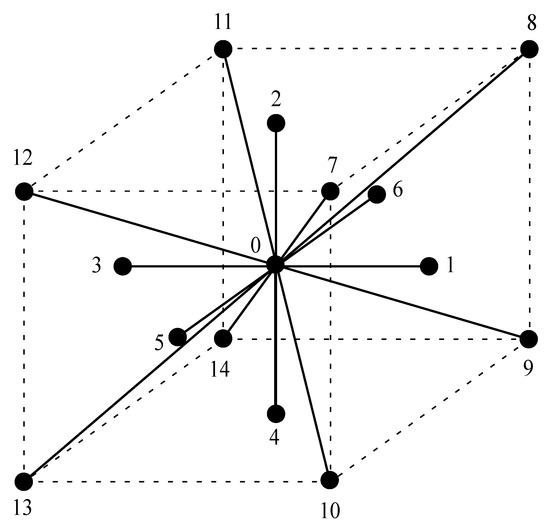
Figure 1.
Discrete velocity set of the D3Q15 model.

Table 1.
Velocity vectors for D3Q15.
Other than velocity vectors, the weighting factor for each direction is necessary for LBM calculation. For the D3Q15 model, the weighting factor is given as follows:
The Boltzmann distribution function is shown by , where f is the number of the collection of the molecules positioned between and with velocities between and at the time t. If the force acts on a molecule with unit mass, the velocity of the molecule changes from to and its position changes from to after undergoing that force. After a collision occurs between particles, f will change in the interval. The rate of change for the distribution function is known as the collision operator shown by (Mohammad [59]). The relationship between distribution functions before and after the collision is given by:
Solving the collision term is very complicated. The popular Bhatnagar, Gross, and Krook (BGK) method (Bhatnagar et al. [60]) for collision operator is used herein. The collision operator is defined as:
where is the relaxation factor and is the equilibrium distribution function. The general form of the equilibrium distribution function can be written as:
where is the macroscopic flow velocity vector, A, B, C, and D are constants and need to be determined based on the conservation principle (mass, momentum, and energy) and is velocity vectors for any of the distribution functions which is introduced in Table 1. The density factor, , is identical to the summation of distribution functions in all directions given by:
The Bhatnagar et al. [60] equilibrium distribution function for fluid can be written as:
in which c is the lattice speed, which is equivalent to the ratio between lattice spacing and lattice time step (x/t). In this research, c is considered equal to 1. Macroscopic properties of the fluid, velocity and pressure p, are calculated as follows:
where is the speed of sound on the lattice and equals to .
Adding an attractive force to the single-phase LBM model makes phase separation into a liquid and its vapor possible. In this study, the multiphase single-component Shan-Chen model [50] is used, which can simulate the behavior of water and air bubbles. No tracking of liquid-vapor interphase is needed in LBM. In the Shan-Chen model, the interaction strength between fluid particles is described by an interparticle potential function. The separation of the liquid and vapor phases occurs naturally in response to the attraction/repulsion force between different phases [61]. The Equation of State (EOS) allows the separation between phases. The Van der Waals EOS was used herein to describe the behavior observed in real gases as:
where P is the gas pressure, V is the gas volume, n is the number of moles, R is gas constant, T is temperature, a is a constant related to the average attraction force between particles, and b is the volume of one mole of particles. The second term on the right-hand side of Equation (9) is an attractive force between molecules. Since a is positive, this term reduces the pressure in comparison to that of a perfect gas. The term in the denominator accounts for the non-negligible volume of molecules. To simulate multiphase fluid and to consider the attraction force, long-range interactions between fluid particles are necessary. The interactions with nearest neighbor particle densities will be sufficient to simulate the basic phenomena of multiphase fluid interactions. For single component multiphase fluids, an attractive (cohesive) force, , between nearest-neighbor fluid particles is needed:
where G is interaction strength factor and is the interaction potential function. A negative G value smaller than −4 indicates an attractive force that separates the fluid into two phases with different densities, including the liquid and vapor [62]. Yuan and Schaefer [63] mentioned that in the coupling of the single component model with the EOS, G becomes unimportant as its effects are canceled out in calculating the force of interaction. In this study, G was set equal to −5.2. According to Shan and Chen [50], the interaction potential function must be monotonically increasing and bounded:
The formulations mentioned above incorporate the molecular attraction aspect of the Van der Waals gas model. For mimicking the attraction force between fluid molecules, should be considered in the BGK operator. The LBM scheme presented for multiphase problems should consider the attractive force such that:
The developed technique by Shan and Chen [50] is a popular method for modeling single-phase multi-component fluid behavior. Numerous studies that were conducted by utilizing Shan and Chen [50] method are in close agreement with analytical and experimental solutions. Some of the recent studies that were conducted by using Shan and Chen [50] method for simulating the behavior of multiphase fluid in porous media are Galindo-Torres et al. [46], Richefeu et al. [48] and Galindo-Torres et al. [47].
The interaction of the fluid and moving solid particles is considered by coupling DEM and LBM. The most simple and common technique for coupling the fluid and solid particles is the bounce-back technique (e.g., [47]). In this technique, particle surface has to be placed halfway between fluid and solid nodes. Even though the bounce-back method is of the first-order in error, lots of researchers are using this technique because of its simplicity. Galindo-Torres et al. [46,47] used the bounce-back boundary conditions for modeling multiphase LBM simulations in a porous medium. The forces and torques applied by the fluid on the solid grains are calculated based on the momentum the fluid exchanges with the solid particles. This method was originally used by Ladd [64] to calculate the forces on solid particles. Based on their study the fluid force is applied through each link connecting fluid node to solid node as:
where is the position of a solid node. The total fluid force (), applied on the particle is sum of the contribution of each link connecting a fluid node to a solid node:
The total torque (), applied on the particle is:
where is a vector connects the particle center to its boundary. The magnitude of the resultant forces is affected by the number of lattice units covered by the solid particle.
2.2. Discrete Element Method
The micro-scale particle displacements and rotations impact the macro-scale response of a granular packing. DEM is an efficient method to model the behavior of granular materials on a micro-scale. In DEM, granular material is modeled as a collection of individual grains (Cundall and Strack [39]). Using DEM makes it possible to trace the movement of every single particle. Contact forces and displacements can be calculated by tracing the movement of individual solid particles. DEM calculations alternate between particles where Newton’s second law is applied and contacts where force-displacement law is used. In this study, other than contact and body forces, fluid forces and torques are acting on every single particle. Newton’s second law determines the motion of every particle under the mentioned loads:
where m is particle mass, is particle position vector, I is particle moment of inertia, is rotational velocity vector, is gravitational acceleration vector, is the inter-particle force at each contact, and is a vector links particle center to the contact location. Momentum exchange between the solid particles and fluid is considered to calculate the applied force and torque. In DEM, solid particles are considered rigid; however, they can overlap. The relationship between relative displacement of two contacting particles and their contact force is generated by force-displacement law. The contact forces are acting in normal and shear directions:
in which and are normal and shear components of the force vector. The normal contact force is defined as:
where is the normal stiffness, and represents the overlap in the normal direction. The shear contact force is computed incrementally according to:
where is the shear stiffness at the contact, and is the shear component of the contact displacement increment vector.
2.3. Computational Scheme
The solution of the coupled response of solid and fluid phases was achieved using an explicit algorithm. The DEM analysis was conducted using the PFC3D software developed by ITASCA [65]. The multiphase fluid code was generated by the authors in C++ and linked to the PFC environment. For solving the coupled model, one time step must be set for each of the solid and the fluid phases. The DEM time step (DEM) corresponds with solid phases and the LBM time step (LBM) corresponds with fluid phases. In order to have a constant time step in DEM, DEM must be chosen to be smaller than the DEM critical time step. The DEM time step is defined to be smaller than the fluid time step LBM. Thus, the fluid time step LBM is equal to DEM, where N is an integer number.
By having this set of time steps, a subcycling time integration for the DEM part is necessary. For every fluid time step, the fluid code receives the location of each particle from the previous DEM time step. After completing the necessary calculations for LBM streaming and LBM collision steps, the hydrodynamic forces and torques are calculated. The DEM code obtains the forces and torques and applies them to the right-hand side of the equations of motion (Equations (16) and (17)). The obtained forces and torques remain constant throughout the subcycling. Finally, particle velocities and locations are obtained using an explicit central finite difference algorithm [65].
3. Model Verification
While there are several publications presenting the effects of desaturation on liquefaction mitigation through 1 g and geotechnical centrifuge experimental results (e.g., [18,19,20,66,67,68,69]), current computational power does not make it practical to have a one-to-one comparison with those experiments. Therefore, two series of verification simulations were performed before running the main model to ensure the LBM code and the coupled LBM-DEM code were without errors. The first series of simulations were modeled to find the relationship between surface tension () and the inverse of the bubble radius (). The second series of simulations were developed to capture the general form of the soil-water characteristic curve in a porous medium.
A spherical light fluid contained in a denser one, which forms a bubble, is affected by inward pressure and outward pressure. The inward pressure works to enlarge the bubble while the outward pressure squeezes it. The surface tension acts as a counterbalancing force to hold the bubble at a constant size. Based on Laplace law, the relationship between the inside and outside pressure difference () and () is a straight line with zero intercept, where the slope of the line represents surface tension. By simulating series of bubbles with different radius sizes, surface tension can be estimated. Figure 2a,b show bubbles with various sizes in the periodic domain. Three-dimensional models were generated in a 100× 100× 100 domain with periodic boundaries. In these models, denser fluid, which represents the surrounding phase, is 20 times heavier than the embraced fluid. Figure 3 presents the plot of vs. in dimensionless lattice units (lu), which is commonly done in LBM simulations (e.g., [46,47,48,61]). LBM lattice units could be transformed to physical units through dimensional analysis [46]. The relationship follows the linear relationship of vs. in Laplace law (Equation (21)) with a slope of 0.095 lu, which corresponds to the surface tension in analyzed fluids:

Figure 2.
Bubbles with different radius, (a) r = 25 and (b) r = 75 , in a 100 × 100 × 100 periodic domain. The yellow color represents the lighter fluid, and the blue color represents the denser fluid.
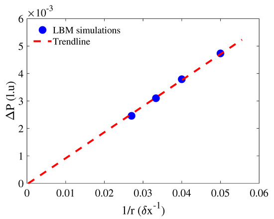
Figure 3.
Linear relation between the pressure difference and the inverse of radius for estimating the surface tension (l.u represents the lattice units).
The relationship between the Laplace pressure difference () and volumetric degree of saturation (S) is also referred to as the water retention curve or the soil-water characteristic curve. Laplace pressure difference (suction), which is defined in Equation (22), is the difference between mean vapor pressure () and mean liquid pressure (). In this paper, mean pressure of the lighter fluid is represented by , and the mean pressure of the denser fluid is shown by :
The soil-water characteristic curve follows a general form where declines in three stages. The first and last steps, where S decreases with lower slope, can be distinguished from the intermediate stage, where S declines rapidly as increases. The general shape of the soil-water characteristic curve was retrieved by the preformed LBM-DEM coupled simulations (Figure 4). A deposit with a smaller height than the one described in Section 4 was used in these simulations. The height of the deposit used herein is one fourth of the height of the deposit described in the next section. The density ratio between the two phases of fluids in the conducted simulations is 20. Here S was calculated as the ratio of the number of LBM nodes occupied by the denser phase to the number of LBM nodes occupied by both fluid phases in the voids.

Figure 4.
Degree of saturation vs. pressure difference between two phases for the analyzed deposit.
4. Simulations
Three granular deposits with different degrees of saturation were generated to study the behavior of unsaturated soils subjected to applied shaking. A one-dimensional basic dynamic excitation in the x-direction was applied to the deposition shown in Figure 5. To model an infinite system, periodic boundary conditions for both liquid and solid phases are established at the lateral boundaries (El Shamy and Abdelhamid [55]). The periodic boundary conditions allow to simulate the huge problem in a limited computational domain. The lower limit is simulated as the liquid tightness limit for both phases. In the solid phase, the base wall mimics the behavior of a solid wall that can move in a horizontal direction. In the liquid phase, the rebound boundary condition is used to simulate the behavior of the solid wall. The constant pressure boundary condition is used to mimic the fluid surface. A semi-infinite deposit was created by solid particles falling under the effect of gravity in a parallelepipedal region with periodic boundaries in the lateral directions. The granular deposit was generated using the underwater bottom density to account for the buoyancy effect on the granules.
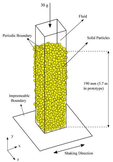
Figure 5.
3-D view of the particle deposit.
Initial sensitivity analysis simulations were performed to assess the spacing between the lattice grid. It was found that the diameter of the bubbles must be greater than 60 LBM nodes to keep the bubbles in a stable size. Considering the computational costs, the size of the generated bubbles are bigger than the solid particles (Figure 6). Essentially one bubble was generated at selected depth locations to yield the targeted degree of saturation (Figure 6). For creating the bubbles, some additional solid particles were generated between the deposit particles by PFC. The centers of the newly added solid particles were used to find the most suitable space between the deposit particles. For the bubbles, lighter fluid was introduced to the LBM model as spheres using the center of those particles. The diameter of these bubbles is covering 60 LBM nodes. After generating the bubbles, the newly added particles were deleted. Note that the location of the bubbles did not remain constant during the simulations. Additionally, the adhesive force between solid particles due to the presence of the fluids was not considered in conducted simulations since these forces tend to be negligible for the simulated range of degrees of saturation. Mei et al. [70] recommended using at least 10 lattice units across the particle diameter. In this study, the average particle diameter is covering 12.5 lattice units.

Figure 6.
2-D cross section showing generated air bubbles at different depth locations: (a) D = 0.6 m, (b) D = 2.7 m and (c) D = 4.8 m for 92% saturated soil deposit at the start of the simulation. The air bubble is represented by white color, solid particles are represented by the yellow color and the liquid is represented by the blue color.
To decrease the number of particles in DEM, the number of nodes in LBM and the duration of the applied shaking, a high gravitation acceleration was applied to the model. The applied high-g level mimics the small scale geotechnical models in centrifuge testing conditions. Table 2 shows the scaling laws utilized to convert different parameters from prototype to model units. In the employed high g-level technique, the scaling factor is only applied to macro-scale parameters, and micro-scale parameters including the average particle diameter are considered identical to the original size in the prototype. This method was found to be a useful technique in DEM simulations to decrease the computational domain to a manageable size in several applications (e.g., [71,72,73]). A summary of computational parameter details and proprieties for solid particles and fluids are listed in Table 3.
Table 2.
Scaling laws used for the conducted simulations.
Table 3.
Simulation details.
The initial permeability of the deposit was estimated by the Kozeny-Carman Equation [74]:
where is the fluid density, r is particle radius, g is the gravitational acceleration, and is the average deposit porosity which is 0.41. The deposit was saturated with a highly viscous fluid to compensate for the effects of the employed 30-g field and large particle sizes (an average diameter of about 6 mm) and comply with the scaling of permeability. For the prototype fluid viscosity of 0.166 Pa.s and the employed particle sizes, the initial permeability of the deposit was estimated to be 2.21 mm/s (same order of coarse sand permeability when saturated with water). The use of much higher viscosity than that of water (166 times higher) compensates for the employed large particle size that would not normally liquefy if it was saturated with water or lightly viscous fluid.
4.1. Computational Details
In the simulations carried out, a deposit of solid particles 190 mm high with lateral dimensions of 50 mm × 50 mm was generated. The pellets had an average diameter of 6 mm with a minimum diameter of 4.8 mm and a maximum diameter of 7.2 mm (Figure 5) and the average saturated density of the deposit was approximately 1967.4 kg/m. The high gravitational acceleration applied to the granular deposit was 30 g. Based on the centrifuge scaling laws (Table 2), the macroscopic length and time scales in the model were 30 times smaller than those in the prototype. As a result, the amplitude of acceleration and the frequency of movement in the model are 30 times higher than in the prototype. The model looks like a prototype where the depth of the granular deposit is 5.7 m.
The one-dimensional dynamic base excitation (in the x-direction) was applied as a velocity-time history to the solid base wall on which the particle deposit rested. The time history of the corresponding acceleration of the dynamic input excitation in the prototype shell is shown in Figure 7. The sinusoidal acceleration input signal is increased gradually until it reaches the maximum amplitude at 4.5 s. It then remained constant for 7.5 s and gradually decreased to zero after 13 s. To estimate the low-stress shear modulus, mean shear wave velocity, and natural frequency of the fully saturated deposit, a sinusoidal fundamental acceleration with an amplitude of 0.01 g and a frequency of 3 was applied to the deposit. Hz under a gravity of 30 g. The acceleration and shear-strain histories were obtained. Using these stories, the low-stress mean shear modulus was found to be about 70 MPa, which corresponds to a mean shear wave velocity of about 187 m/s. Therefore, the natural frequency of the deposit (defined as the shear wave velocity divided by four times the height of the deposit) was approximately 8.2 Hz.

Figure 7.
Applied shake to the base wall of the granular deposit.
The results of models with 100%, 92%, and 82% of the degree of saturation were analyzed. Several parameters were monitored at a time interval of 0.000016 s in the model (0.0048 s in prototype) during the simulations. These parameters include the vertical effective stress, excess pore-pressure ratio, coordination number, shear stress–strain time histories, and averaged particle acceleration. Results are presented in prototype units unless otherwise specified.
4.2. Simulation Results
Excess pore pressure ratio (ratio of fluid pore pressure increase to initial effective vertical stress) and effective stress-time histories were used to identify liquefaction from a large-scale perspective. The accumulation of an excessive pore pressure ratio was the key factor in identifying the initiation of liquefaction. In general, liquefaction has been defined as the moment when the pore pressure ratio reaches the value one. At this time, the contact forces between the particles have approached zero and therefore the effective stress has disappeared. The temporal evolutions of the pore pressure ratio at selected depth locations for models with different degrees of saturation are shown in Figure 8. The results show that the pore pressure ratio approached values between 0.8 and 1 in the upper 2.7 m of the fully saturated deposit. In the deepest parts of the fully saturated deposit, the pore pressure ratio remained around 0.8.

Figure 8.
Time histories of the excess pore pressure ratio at selected depth locations for soil deposits with different degrees of saturation.
Based on the simulations performed, liquefaction occurred at the fully saturated deposit. In the desaturated deposits, this ratio remained below 0.5 for all levels, despite the increase in the pore pressure ratio at shallow places (Figure 8). No liquefaction was observed at any depth in the 82% and 92% saturated deposit. It can also be concluded that the decrease in the degree of saturation from 100% to 92% has a significant impact on the decrease in the pore pressure ratio. However, further reducing the saturation level from 92% to 82% has less significant effects. This answer shows that a small percentage reduction in the degree of saturation has a significant effect on reducing the risk of liquefaction. The same behavior was observed in several experimental studies (e.g., [18,19,20]). It should be noted, however, that most of these experimental studies showed a considerable difference in behavior as the degree of saturation decreased say from ∼95% to ∼85%, which was not observed in current simulations. This could be attributed to the testing environment that imposes undrained conditions in the experiments while this condition is not enforced in the presented LBM-DEM model. On the other hand, the field study reported by [23] showed that no significant difference was observed regarding the increase in liquefaction resistance for the degrees of saturation of about 88∼94%. Similarly, the free-field results of the centrifuge experiments performed by [68] showed no significant difference between the response at the degrees of saturation of 93.5% and 79.5%. The results of the in situ testing and centrifuge experiments, which are in agreement with the results from performed simulations, highlight the importance of system level modeling as opposed to element level testing.
Liquefaction is also marked when the vertical effective stress of the soil decreases to zero. The vertical effective stress of the fully saturated deposit declined and approached zero at all depth locations. The reduction in the vertical effective stress was significantly lower in the desaturated deposits compared to the fully saturated one (Figure 9). There is not a significant distinction between the vertical effective stress time histories of the desaturated deposits as can be seen in Figure 9.

Figure 9.
Time histories of the vertical effective stress at selected depth locations for soil deposits with different degrees of saturation.
During liquefaction, the shear moduli of the granular soil approached zero as a result of the vanishing effective stress. The shear stress–strain loops for the deposits at selected depth locations are shown in Figure 10. The shear stress–strain loops show a stiffness degradation of shear moduli at different depths of the deposits with different degrees of saturation during shaking. The shear modulus of the fully saturated deposit approaches smaller values in comparison with the desaturated deposits. Shear modulus reduction curves for soil deposits with different degrees of saturation are shown in Figure 11. The reduction in shear modulus in the desaturated deposits is mainly due to the experienced large shear strains. However, the degradation of the shear modulus in the saturated deposit is due to the combined effect of pore pressure buildup and subsequent decrease in shear stress as well as the large shear strains experienced by the deposit.

Figure 10.
Shear stress–strain loops at selected depth locations for soil deposits with different degrees of saturation.

Figure 11.
Shear modulus reduction curve for soil deposits with different degrees of saturation at D = 2.7 m.
Figure 12 shows the settlement time histories in the conducted simulations. There is not a significant difference between the final settlements and settlement time histories of the deposits with various degrees of saturation. Even though the reduction in porosity causes the pore-pressure buildup and, consequently lead to liquefaction, there is not a significant difference between the settlement time histories of the liquefied and desaturated granular deposits. It can be concluded that the main reason for the settlement in the simulated deposits was the applied shaking and not liquefaction of the deposit.

Figure 12.
Settlement time histories for soil deposits with different degrees of saturation.
It was of importance to examine the averaged acceleration in the shaking direction of the solid particles at each depth location (Figure 13). The behavior of acceleration time history presents the resisting force to the motion of the solid particles during shaking. As the soil liquefies, particle contacts are lost and smaller acceleration amplitudes are transmitted throughout the liquefied portion of the deposit (Figure 13a). As with the other evaluated parameters, there is not an apparent difference between the acceleration time histories of the desaturated deposits (Figure 13b,c).

Figure 13.
Acceleration time histories at selected depth locations for soil deposits with different degrees of saturation (a) Fully saturated, (b) S = 92% and (c) S = 82%.
The degree of saturation variation during shaking at different depth locations of desaturated deposits is shown in Figure 14. In general, the degree of saturation was not constant with depth, and its local value changed with time as the bubbles moved up and down and were squeezed during shaking. The averaged degree of saturation variation of the deposits during the shaking is shown in Figure 15. There is a small increase in the degree of saturation for both desaturated deposits. This increase of the degree of saturation represents the volume reduction of the air bubbles during the cyclic loading. The air bubbles volume reduction is happening because they absorb the excess pore pressure generated during shaking. From the micro-scale point of view, liquefaction occurs at the locations where the coordination number of the solid particles (the average number of contacts per particle) reduces until they start floating. In order to have a stable pack of frictional spheres, the coordination number is required to remain 4 or above (Edwards [75]). Figure 16 shows the coordination number time histories of the deposits with different degrees of saturation. The top 0.6 m of the fully saturated soil deposit, coordination number dropped significantly to a value below 4. The 2.7 m and 4.8 m depth locations of the fully saturated deposit the coordination number was sustained above 3, but below the value of 4. This response shows that instability occurred in every depth locations of the fully saturated deposit. Figure 16 also shows that the coordination numbers in the 82% and 92% saturated deposits remained virtually constant. This behavior confirms that liquefaction was not observed at any depth location in the desaturated deposits. Coordination number time histories for both desaturated deposits were almost identical during the applied shaking. It can be concluded that the decrement of the degree of saturation from 92% to 82% does not have a significant effect on the coordination number time history. The coordination number time history is affected distinctly when the degree of saturation drops from 100% to 92%.

Figure 14.
Degree of saturation at different elevations for desaturated soil deposits during the shaking (a) S = 92% and (b) S = 82%.

Figure 15.
Degree of saturation change during the shaking for desaturated soil deposits (Dashed lines represent the initial degree of saturation of the deposits).

Figure 16.
Time histories of the coordination number at selected depth locations for soil deposits with different degrees of saturation.
5. Conclusions
This work investigates the potential of a three-dimensional pore model developed to analyze liquefaction in fully desaturated granular deposits under seismic excitation. The multiphase single-component lattice Boltzmann method was used to model the liquid phase at the pore scale, while the solid phase was idealized at the microscale using the discrete element method. The presented coupled LBM-DEM model considers the discrete behavior of granular particles, including the actual fluid flow in the pore space. The forces exerted on the solid particles by the fluid phase were calculated by considering the exchange of momentum between the solid particles and the fluid. The model was used to simulate the response of soil deposits with different degrees of saturation during seismic excitation. Three granular deposits subjected to dynamic excitation with saturation degrees of 100%, 92% and 82% were modeled.
Based on the results of the simulations carried out, liquefaction took place in the fully saturated granular deposit. For the same set of conditions applied for the fully saturated deposit, no liquefaction was observed at any depth location of the unsaturated deposits. It has also been noted that reducing the degree of saturation from 100% to 92% primarily affects behavior. At the depth near-surface location, the excess pore pressure ratio dropped from near 1 to less than 0.4. Furthermore, at the deepest points of the 92% saturated deposit, a significant drop in the pore pressure ratio in excess of the values observed in the fully saturated deposit was observed.
A significant behavior change was observed in the effective stress time histories after inducing the bubbles to the fully saturated deposit. Acceleration amplitude increased by desaturating the fully saturated deposit during shaking in all depth locations. Shear modulus approached higher values in the 92% saturated deposit in comparison to the fully saturated one for a specific shear strain. Further reduction in the degree of saturation from 92% to 82% did not have a significant effect on the computed parameters. Similar behavior was observed for the time history of the coordination number. Coordination number time history was affected significantly by an 8% decrease of the degree of saturation in the fully saturated deposit. However, it remained close to the value of 4 in both 82% and 92% saturated deposits. No significant difference was observed between the settlement time history and the final settlement of the granular deposits with different degrees of saturation. The volume reduction due to the dynamic excitation was the leading cause of the settlement and not liquefaction.
Because of the high cost of the computational scheme, simulating the practical size of the solid particles and air bubbles was not feasible herein. However, with the current increasing trend of high performance computing platforms that utilizes parallel computing, there is high potential for the presented technique to model systems of actual particle and bubble sizes.
Author Contributions
A.N.: Software, Formal analysis, Data curation, Visualization, Writing—Original draft preparation. U.E.S.: Conceptualization, Methodology, Investigation, Supervision, Writing—Editing. All authors have read and agreed to the published version of the manuscript.
Funding
There was no external funding for this project.
Informed Consent Statement
The software employed in this study is the commercial software PFC3D [65]. The code for modeling LBM and coupling with DEM was written in C++ and compiled with PFC3D.
Data Availability Statement
Input and output data for conducted simulations is available upon reasonable request to the corresponding author.
Conflicts of Interest
The authors declare that they have no known competing financial interests or personal relationships that could have appeared to influence the work reported in this paper.
References
- Lukas, R.G. Dynamic Compaction for Highway Construction; US Department of Transportation, Federal Highway Administration: Washington, DC, USA, 1986. [Google Scholar]
- Dise, K.; Stevens, M.G.; Von Thun, J.L. Dynamic compaction to remediate liquefiable embankment foundation soils. In In-Situ Deep Soil Improvement; ASCE: Reston, VA, USA, 1994; pp. 1–25. [Google Scholar]
- Lukas, R. Geotechnical Engineering Circular No. 1-Dynamic Compaction; Technical Report; United States Federal Highway Administration: Washington, DC, USA, 1995. [Google Scholar]
- Andrus, R.D.; Chung, R.M. Ground Improvement Techniques for Liquefaction Remediation Near Existing Lifelines; US National Institute of Standards and Technology: Gaithersburg, MD, USA, 1995. [Google Scholar]
- Mitchell, J.K.; Christopher, D.P.B.; Munson, T.C. Performance of improved ground during earthquakes. In Soil Improvement for Earthquake Hazard Mitigation; ASCE: Reston, VA, USA, 1995; pp. 1–36. [Google Scholar]
- Boulanger, R.W.; Hayden, R.F. Aspects of compaction grouting of liquefiable soil. J. Geotech. Eng. 1995, 121, 844–855. [Google Scholar] [CrossRef]
- Martin, J.R.; Olgun, C.G.; Mitchell, J.K.; Durgunoglu, H.T. High-modulus columns for liquefaction mitigation. J. Geotech. Geoenviron. Eng. 2004, 130, 561–571. [Google Scholar] [CrossRef]
- Gallagher, P.M.; Conlee, C.T.; Rollins, K.M. Full-scale field testing of colloidal silica grouting for mitigation of liquefaction risk. J. Geotech. Geoenviron. Eng. 2007, 133, 186–196. [Google Scholar] [CrossRef]
- El Mohtar, C.S.; Bobet, A.; Santagata, M.C.; Drnevich, V.P.; Johnston, C.T. Liquefaction mitigation using bentonite suspensions. J. Geotech. Geoenviron. Eng. 2012, 139, 1369–1380. [Google Scholar] [CrossRef]
- O’rourke, T.D.; Goh, S.H. Reduction of liquefaction hazards by deep soil mixing. In Post-Earthquake Reconstruction Strategies: NCEER-INCEDE Center-to-Center Project; National Science Foundation: Alexandria, VA, USA, 1997; pp. 87–105. [Google Scholar]
- Holm, G. Keynote lecture: Applications of dry mix methods for deep soil stabilization. In Dry Mix Methods for Deep Soil Stabilization; Routledge: London, UK, 1999; pp. 13–15. [Google Scholar]
- Porbaha, A.; Zen, K.; Kobayashi, M. Deep mixing technology for liquefaction mitigation. J. Infrastruct. Syst. 1999, 5, 21–34. [Google Scholar] [CrossRef]
- Seed, H.B.; Booker, J.R. Stabilization of potentially liquefiable sand deposits using gravel drains. J. Geotech. Geoenviron. Eng. 1977, 103, 13050. [Google Scholar] [CrossRef]
- Ishihara, K.; Yamazaki, F. Cyclic simple shear tests on saturated sand in multi-directional loading. Soils Found. 1980, 20, 45–59. [Google Scholar] [CrossRef]
- Tokimatsu, K.; Yoshimi, Y. Effects of vertical drains on the bearing capacity of saturated sand during earthquakes. In Proceedings of the Engineering for Protection from Natural Disasters, Bangkok, Thailand, 7–9 January 1980. [Google Scholar]
- Boulanger, R.W.; Idriss, I.M.; Stewart, D.P.; Hashash, Y.; Schmidt, B. Drainage capacity of stone columns or gravel drains for mitigating liquefaction. In Drainage Capacity of Stone Columns or Gravel Drains for Mitigating Liquefaction; American Society of Civil Engineers: Reston, VA, USA, 1998; pp. 678–690. [Google Scholar]
- DeJong, J.T.; Fritzges, M.B.; Nüsslein, K. Microbially induced cementation to control sand response to undrained shear. J. Geotech. Geoenviron. Eng. 2006, 132, 1381–1392. [Google Scholar] [CrossRef]
- Martin, G.R.; Finn, W.D.L.; Seed, H.B. Fundementals of liquefaction under cyclic loading. J. Geotech. Geoenviron. Eng. 1975, 101, 11231. [Google Scholar]
- Chaney, R.C. Saturation effects on the cyclic strength of sands. In Proceedings of the ASCE Geotechnical Engineering Division Specialty Conference, Pasadena, CA, USA, 19–21 June 1978. [Google Scholar]
- Yoshimi, Y.; Tanaka, K.; Tokimatsu, K. Liquefaction resistance of a partially saturated sand. Soils Found. 1989, 29, 157–162. [Google Scholar] [CrossRef]
- Okamura, M.; Ishihara, M.; Tamura, K. Degree of saturation and liquefaction resistances of sand improved with sand compaction pile. J. Geotech. Geoenviron. Eng. 2006, 132, 258–264. [Google Scholar] [CrossRef]
- Yegian, M.K.; Eseller-Bayat, E.; Alshawabkeh, A.; Ali, S. Induced-partial saturation for liquefaction mitigation: Experimental investigation. J. Geotech. Geoenviron. Eng. 2007, 133, 372–380. [Google Scholar] [CrossRef]
- Okamura, M.; Takebayashi, M.; Nishida, K.; Fujii, N.; Jinguji, M.; Imasato, T.; Yasuhara, H.; Nakagawa, E. In-situ desaturation test by air injection and its evaluation through field monitoring and multiphase flow simulation. J. Geotech. Geoenviron. Eng. 2011, 137, 643–652. [Google Scholar] [CrossRef]
- Eseller-Bayat, E.; Yegian, M.K.; Alshawabkeh, A.; Gokyer, S. Liquefaction response of partially saturated sands. i: Experimental results. J. Geotech. Geoenviron. Eng. 2012, 139, 863–871. [Google Scholar] [CrossRef]
- Dafalias, Y. Bounding surface formulation of soil plasticity. In Soil Mechanics-Transient and Cyclic Loads; Wiley: New York, NJ, USA, 1982; pp. 253–282. [Google Scholar]
- Desai, C.S.; Siriwardane, H.J. Constitutive Laws for Engineering Materials with Emphasis on Geologic Materials; Prentice-Hall: Hoboken, NJ, USA, 1984. [Google Scholar]
- Wood, D.M. Soil Behaviour and Critical State Soil Mechanics; Cambridge University Press: Cambridge, UK, 1990. [Google Scholar]
- Madabhushi, S.P.G.; Zeng, X. Seismic response of gravity quay walls. ii: Numerical modeling. J. Geotech. Geoenviron. Eng. 1998, 124, 418–427. [Google Scholar] [CrossRef]
- Borja, R.I.; Chao, H.-Y.; Montáns, F.J.; Lin, C.-H. Ssi effects on ground motion at lotung lsst site. J. Geotech. Geoenviron. Eng. 1999, 125, 760–770. [Google Scholar] [CrossRef]
- Regueiro, R.A.; Borja, R.I. A finite element model of localized deformation in frictional materials taking a strong discontinuity approach. Finite Elem. Anal. Des. 1999, 33, 283–315. [Google Scholar] [CrossRef]
- Seid-Karbasi, M.; Byrne, P.M. Seismic liquefaction, lateral spreading, and flow slides: A numerical investigation into void redistribution. Can. Geotech. J. 2007, 44, 873–890. [Google Scholar] [CrossRef]
- Andrade, J. A predictive framework for liquefaction instability. Géotechnique 2009, 59, 673–682. [Google Scholar] [CrossRef]
- Bian, H.; Shahrour, I. Numerical model for unsaturated sandy soils under cyclic loading: Application to liquefaction. Soil Dyn. Earthq. Eng. 2009, 29, 237–244. [Google Scholar] [CrossRef]
- Buscarnera, G.; Di Prisco, C. Soil stability and flow slides in unsaturated shallow slopes: Can saturation events trigger liquefaction processes. Géotechnique 2013, 63, 801–817. [Google Scholar] [CrossRef]
- Liu, C.; Muraleetharan, K.K. Numerical study on effects of initial state on liquefaction of unsaturated soils. In Proceedings of the GeoCongress 2012: State of the Art and Practice in Geotechnical Engineering, Oakland, CA, USA, 25–29 March 2012; pp. 2432–2441. [Google Scholar]
- Zhang, B.; Muraleetharan, K.K. Implementation of a hydromechanical elastoplastic constitutive model for fully coupled dynamic analysis of unsaturated soils and its validation using centrifuge test results. Acta Geotech. 2019, 14, 327–360. [Google Scholar] [CrossRef]
- Vecchia, G.D.; Cremonesi, M.; Pisanò, F. On the rheological characterisation of liquefied sands through the dam-breaking test. Int. J. Numer. Anal. Methods Geomech. 2019, 43, 1410–1425. [Google Scholar] [CrossRef]
- Cundall, P.A. A computer model for simulating progressive large scale movements in blocky rock systems. In Proceedings of the Symposium of the International Society of Rock Mechanics, Nancy, France, 4–6 October 1971; Volume 1, pp. 1671–1676. [Google Scholar]
- Cundall, P.A.; Strack, O. A discrete numerical model for granular assemblies. Ge´otechnique 1979, 29, 47–65. [Google Scholar] [CrossRef]
- Schenkengel, K.-U.; Vrettos, C. Simulation of liquefied sand by the lattice boltzmann method. Geotechnik 2014, 37, 96–104. [Google Scholar] [CrossRef]
- Buckles, J.J.; Hazlett, R.D.; Chen, S.; Eggert, K.G.; Grunau, D.W.; Soll, W.E. Toward improved prediction of reservoir flow performance. Los Alamos Sci. 1994, 22, 112–121. [Google Scholar]
- Shan, H.; Chen, X. Lattice boltzmann model for simulating flows with multiple phases and components. Phys. Rev. E 1993, 47, 1815. [Google Scholar] [CrossRef]
- Shan, X.; Doolen, G. Multicomponent lattice-boltzmann model with interparticle interaction. J. Stat. Phys. 1995, 81, 379–393. [Google Scholar] [CrossRef]
- Martys, N.S.; Chen, H. Simulation of multicomponent fluids in complex three-dimensional geometries by the lattice boltzmann method. Phys. Rev. E 1996, 53, 743. [Google Scholar] [CrossRef]
- Sukop, M.C.; Huang, H.; Lin, C.L.; Deo, M.D.; Oh, K.; Miller, J.D. Distribution of multiphase fluids in porous media: Comparison between lattice boltzmann modeling and micro-x-ray tomography. Phys. Rev. E 2008, 77, 026710. [Google Scholar] [CrossRef]
- Galindo-Torres, S.A.; Scheuermann, A.; Li, L.; Pedroso, D.M.; Williams, D.J. A lattice boltzmann model for studying transient effects during imbibition–drainage cycles in unsaturated soils. Comput. Phys. Commun. 2013, 184, 1086–1093. [Google Scholar] [CrossRef]
- Galindo-Torres, S.A.; Scheuermann, A.; Li, L. Boundary effects on the soil water characteristic curves obtained from lattice boltzmann simulations. Comput. Geotech. 2016, 71, 136–146. [Google Scholar] [CrossRef]
- Richefeu, V.; Radjai, F.; Delenne, J.Y. Lattice boltzmann modelling of liquid distribution in unsaturated granular media. Comput. Geotech. 2016, 80, 353–359. [Google Scholar] [CrossRef]
- Grunau, D.; Chen, S.; Eggert, K. A lattice boltzmann model for multiphase fluid flows. Phys. Fluids A Fluid Dyn. 1993, 5, 2557–2562. [Google Scholar] [CrossRef]
- Shan, X.; Chen, H. Simulation of nonideal gases and liquid-gas phase transitions by the lattice boltzmann equation. Phys. Rev. E 1994, 49, 2941. [Google Scholar] [CrossRef]
- Huang, H.; Li, Z.; Liu, S.; Lu, X.-Y. Shan-and-chen-type multiphase lattice boltzmann study of viscous coupling effects for two-phase flow in porous media. Int. J. Numer. Methods Fluids 2009, 61, 341–354. [Google Scholar] [CrossRef]
- Eshghinejadfard, A.; Daróczy, L.; Janiga, G.; Thévenin, D. Calculation of the permeability in porous media using the lattice boltzmann method. Int. J. Heat Fluid Flow 2016, 62, 93–103. [Google Scholar] [CrossRef]
- Han, Y.; Cundall, P.A. Lbm–dem modeling of fluid–solid interaction in porous media. Int. J. Numer. Anal. Methods Geomech. 2013, 37, 1391–1407. [Google Scholar] [CrossRef]
- Abdelhamid, Y.; El Shamy, U. Pore-scale modeling of surface erosion in a particle bed. Int. J. Numer. Anal. Methods Geomech. 2014, 38, 142–166. [Google Scholar] [CrossRef]
- El Shamy, U.; Abdelhamid, Y. Modeling granular soils liquefaction using coupled lattice boltzmann method and discrete element method. Soil Dyn. Earthq. Eng. 2014, 67, 119–132. [Google Scholar] [CrossRef]
- Abdelhamid, Y.; El Shamy, U. Pore-scale modeling of fine-particle migration in granular filters. Int. J. Geomech. 2015, 16, 04015086. [Google Scholar] [CrossRef]
- Qiu, L. A coupling model of dem and lbm for fluid flow through porous media. Procedia Eng. 2015, 102, 1520–1525. [Google Scholar] [CrossRef]
- El Shamy, U.; Abdelhamid, Y. Some aspects of the impact of multidirectional shaking on liquefaction of level and sloping granular deposits. J. Eng. Mech. 2016, 143, C4016003. [Google Scholar] [CrossRef]
- Mohammad, A.A. Lattice Boltzmann Method Fundamentals and Engineering Applications with Computer Codes; Springer: Berlin/Heidelberg, Germany, 2011; Volume 1. [Google Scholar]
- Bhatnagar, P.L.; Gross, E.P.; Krook, M. A model for collision processes in gases. i. small amplitude processes in charged and neutral one-component systems. Phys. Rev. 1954, 94, 511. [Google Scholar] [CrossRef]
- Peng, C.; Tian, S.; Li, G.; Sukop, M.C. Simulation of multiple cavitation bubbles interaction with single-component multiphase lattice boltzmann method. Int. J. Heat Mass Transf. 2019, 137, 301–317. [Google Scholar] [CrossRef]
- Baakeem, S.S.; Bawazeer, S.A.; Mohamad, A.A. Comparison and evaluation of shan–chen model and most commonly used equations of state in multiphase lattice boltzmann method. Int. J. Multiph. Flow 2020, 128, 103290. [Google Scholar] [CrossRef]
- Yuan, P.; Schaefer, L. Equations of state in a lattice boltzmann model. Phys. Fluids 2006, 18, 042101. [Google Scholar] [CrossRef]
- Ladd, A.J.C. Numerical simulations of particulate suspensions via a discretized boltzmann equation. Part 1. Theoretical foundation. J. Fluid Mech. 1994, 271, 285–309. [Google Scholar] [CrossRef]
- ITASCA. PFC3D: Particle Flow Code in 3 Dimensions Version 4.0; US Minneapolis-Itasca Consulting Group, Inc.: Minneapolis, MN, USA, 2008. [Google Scholar]
- Ghayoomi, M.; McCartney, J.; Ko, H.-Y. Centrifuge test to assess the seismic compression of partially saturated sand layers. Geotech. Test. J. 2011, 34, 321–331. [Google Scholar]
- Ravichandran, N.; Krishnapillai, S.H.; Machmer, B. A novel procedure for physical modeling of unsaturated soil-pile system using geotechnical centrifuge. J. Earth Sci. Geotech. Eng. 2013, 3, 119–134. [Google Scholar]
- Zeybek, A.; Madabhushi, S.P.G. Centrifuge testing to evaluate the liquefaction response of air-injected partially saturated soils beneath shallow foundations. Bull. Earthq. Eng. 2017, 15, 339–356. [Google Scholar] [CrossRef]
- Mirshekari, M.; Ghayoomi, M. Centrifuge tests to assess seismic site response of partially saturated sand layers. Soil Dyn. Earthq. Eng. 2017, 94, 254–265. [Google Scholar] [CrossRef]
- Mei, R.; Yu, D.; Shyy, W.; Luo, L.-S. Force evaluation in the lattice boltzmann method involving curved geometry. Phys. Rev. E 2002, 65, 041203. [Google Scholar] [CrossRef]
- El Shamy, U. A Coupled Continuum-Discrete Fluid-Particle Model for Granular Soil Liquefaction. Ph.D. Thesis, Rensselaer Polytechnic Institute, Troy, NY, USA, 2004. [Google Scholar]
- El Shamy, U.; Zeghal, M.; Dobry, R.; Thevanayagam, S.; Elgamal, A.; Abdoun, T.; Medina, C.; Bethapudi, R.; Bennett, V. Micromechanical aspects of liquefaction-induced lateral spreading. Int. J. Geomech. 2010, 10, 190–201. [Google Scholar] [CrossRef]
- El Shamy, U.; Aydin, F. Multiscale modeling of flood-induced piping in river levees. J. Geotech. Geoenviron. Eng. 2008, 134, 1385–1398. [Google Scholar] [CrossRef]
- Carman, P.C. Fluid flow through granular beds. Trans. Inst. Chem. Eng. 1937, 15, 150–166. [Google Scholar] [CrossRef]
- Edwards, S.F. The equations of stress in a granular material. Phys. A Stat. Mech. Its Appl. 1998, 249, 226–231. [Google Scholar] [CrossRef]


Disclaimer/Publisher’s Note: The statements, opinions and data contained in all publications are solely those of the individual author(s) and contributor(s) and not of MDPI and/or the editor(s). MDPI and/or the editor(s) disclaim responsibility for any injury to people or property resulting from any ideas, methods, instructions or products referred to in the content. |
© 2022 by the authors. Licensee MDPI, Basel, Switzerland. This article is an open access article distributed under the terms and conditions of the Creative Commons Attribution (CC BY) license (https://creativecommons.org/licenses/by/4.0/).