Article

Dynamic Modeling of Inland Flooding and Storm Surge on Coastal Cities under Climate Change Scenarios: Transportation Infrastructure Impacts in Norfolk, Virginia USA as a Case Study

1
Department of Engineering Systems and Environment, University of Virginia, Olsson Hall, Charlottesville, VA 22904, USA
2
Department of Civil and Environmental Engineering, Old Dominion University, Norfolk, VA 23529, USA
3
Irrigation and Hydraulics Engineering Department, Faculty of Engineering, Cairo University, Giza 12614, Egypt
4
BTM WBM Pty Ltd., Level 8, 200 Creek Street, Brisbane 4000, Australia
*
Author to whom correspondence should be addressed.
Geosciences 2022, 12(6), 224; https://doi.org/10.3390/geosciences12060224
Submission received: 20 March 2022 / Revised: 10 May 2022 / Accepted: 23 May 2022 / Published: 25 May 2022
(This article belongs to the Special Issue Flood Hazard and Risk in Urban Areas)

Abstract

:
Low-lying coastal cities across the world are vulnerable to the combined impact of rainfall and storm tide. However, existing approaches lack the ability to model the combined effect of these flood mechanisms, especially under climate change and sea level rise (SLR). Thus, to increase flood resilience of coastal cities, modeling techniques to improve the understanding and prediction of the combined effect of these flood hazards are critical. To address this need, this study presents a modeling system for assessing the combined flood impact on coastal cities under selected future climate scenarios that leverages ocean modeling with land surface modeling capable of resolving urban drainage infrastructure within the city. The modeling approach is demonstrated in quantifying the impact of possible future climate scenarios on transportation infrastructure within Norfolk, Virginia, USA. A series of combined storm events are modeled for current (2020) and projected future (2070) climate scenarios. The results show that pluvial flooding causes a larger interruption to the transportation network compared to tidal flooding under current climate conditions. By 2070, however, tidal flooding will be the dominant flooding mechanism with even nuisance flooding expected to happen daily due to SLR. In 2070, nuisance flooding is expected to cause a 4.6% total link close time (TLC), which is more than two times that of a 50-year storm surge (1.8% TLC) in 2020. The coupled flood model was compared with a widely used but physically simplistic bathtub method to assess the difference resulting from the more complex modeling presented in this study. The results show that the bathtub method overestimated the flooded area near the shoreline by 9.5% and 3.1% for a 10-year storm surge event in 2020 and 2070, respectively, but underestimated the flooded area in the inland region by 9.0% and 4.0% for the same events. The findings demonstrate the benefit of sophisticated modeling methods compared to more simplistic bathtub approaches, in climate adaptive planning and policy in coastal communities.

1. Introduction

Coastal cities are increasingly vulnerable to flooding exposure owing to the growing population, urbanization, climate change, and relative sea level rise (SLR) [1,2,3,4,5]. Flooding can be destructive in these low-lying, densely populated, and highly developed regions [6,7]. For example, Hurricanes Katrina (2005), Sandy (2012), Harvey (2017), and Florence (2019) caused significant loss of life and damage on the U.S. Gulf and Atlantic Coasts. According to Hanson et al. (2010) [1], about 40 million people were exposed to a 100-year coastal flood event in the 136 largest port cities in the world in 2005. By the 2070s, the population exposed to such an event could increase threefold. Hallegatte et al. [2] estimated flood losses in a single year by 2050 to be more than 10 times those in 2005. Despite facing these hazards, protection measures in coastal cities have often been inadequate [8], primarily due to short-term economic decisions and the uncertainty of future risk [3]. Therefore, to help inform policy decisions, it is necessary to enhance the understanding and modeling capacities for assessing flood hazards in coastal cities under a changing climate.
Individual flood mechanisms, such as pluvial flooding and tidal flooding, can cause widespread impacts in coastal cities [9]. However, if multiple mechanisms occur concurrently, flood severity can be greatly exacerbated [10,11,12,13]. Prior studies have demonstrated the statistical dependence of rainfall and storm tide in coastal regions [11,12,14]. Batten et al. [12] analyzed the temporal dependence of rainfall and storm tide in Virginia Beach, Virginia, and found that the correlation coefficients between rainfall and storm tide vary between 0.336 and 0.452 across different data sources. Meanwhile, they indicated that over half of the rainfall events occurred while the tide level was higher than the average high tide. Wahl et al. [11] estimated the likelihood of a joint occurrence of rainfall and storm tide across the contiguous United States (US) Coast and concluded that the possibility of a compound storm is higher on the Atlantic/Gulf Coast than on the Pacific Coast. Meanwhile, they found that the frequency of compound storms has significantly increased in the past century, and this trend is expected to continue due to climate change. Xu et al. [14] estimated the bivariate return periods of compound rainfall and storm tide based on copula functions and failure probability and showed significant correlation between rainfall and storm tide.
Given the correlation between storm tide and rainfall, considerable efforts have been made to develop methodologies for modeling the combined impact from these flood mechanisms. In prior works, the proposed modeling systems are normally the coupling of a one-dimensional (1D: [7,15,16]) or two-dimensional (2D: [17,18,19]) overland model with a 2D or three-dimensional (3D) storm surge model (e.g., ADCRIC, MIKE21, and Delft3D). Yin [17] proposed a coastal inundation model by coupling a storm surge model (ADCIRC) with an urban flood model (FloodMap). At the city scale, the coupled model demonstrates improved results over ADCIRC modeling alone for both flood extent and depth. In Silva-Araya et al. (2018) [18], a 2D hydrologic model was coupled with a 2D storm surge model for Puerto Rico. In an execution, the storm surge model will run first to prepare a tidal boundary for the hydrologic model. The results show that the interaction between pluvial flooding and tidal flooding caused increased flooding compared to a storm surge alone. Coastal regions are often located in low-relief terrain without a large amount of storage potential. Furthermore, the topography complexity increases significantly in urban environments due to the surface and subsurface infrastructure. Routing water in such environments requires high-resolution 2D hydrodynamic formulation to model the complex street-level overland flooding ([7,13]). In urban environments, subsurface drainage systems play a key role in managing urban flooding, and their capacity can be significantly influenced by downstream tidal boundary conditions. However, in prior work, subsurface drainage systems are often not explicitly included in modeling combined coastal flooding ([17,18]). This is primarily due to the difficulty in obtaining a large-scale drainage system database in order to parameterize the model. Without explicitly including subsurface drainage systems, flood models may inaccurately estimate the effect of not only pluvial flooding, but also tidal flooding due to the backing up of ocean water into the city through storm drainage pipes during storm surge events. Therefore, to increase the accuracy of coastal city flooding, this study used an overland flood model consisting of a large-scale 1D subsurface drainage network and a 2D surface overland hydrodynamic model. This model system is capable of simulating the dynamics of surface runoff and pipe flow, as well as the interaction between them. The model was then coupled with a physics-based storm surge model built in [20] to obtain ocean boundary conditions. This coupled modeling system provides a powerful tool to explore the impact of flooding on a complex physical system under both current climate conditions and future climate scenarios. Model outputs with a high spatial-temporal resolution can be applied to investigate the flood impact at a street-scale, which is needed for flood mitigation and engineering design under climate change.
Methodologies with varying complexities have been developed in prior works to estimate the flood impact on critical infrastructure systems such as transportation infrastructure under climate change and SLR [17,21,22,23,24]. One simplified approach, the so called “bathtub” method, assumes that the water surface is level so that flood inundation can be easily estimated by using a digital elevation model (DEM). Because of its algorithmic simplicity and computational efficiency, the bathtub method is commonly applied to evaluate the impact of SLR and/or a storm surge in coastal environments. Sadler et al. [23], for example, used the bathtub method and traffic information to identify critical roadways in Norfolk and Virginia Beach, Virginia exposed to future flood hazards. A similar method was adopted by [25] to assess the increasing vulnerability of roadways to nuisance flooding on the U.S. east coast. While the bathtub method is convenient, past studies suggest that it tends to overestimate flood depths and extents because of its physical oversimplification of flood routing [26,27].
The objective of this study, therefore, is to advance methods for modeling the combined impact of rainfall and storm tide in coastal cities under selected future climate scenarios. As a demonstration, the method was applied to a portion of Norfolk, Virginia to assess the flood impact on the transportation network for a series of storm scenarios under the current climate conditions and possible future climate scenarios. The results are compared to the widely used bathtub approach to quantify the advantage of complex dynamic flood models in coastal urban environments. The main contribution of this study, therefore, is to advance the method for dynamically modeling the combined impact of rainfall and storm tide in coastal cities and demonstrate the application of this method in assessing flooding impact under both the current climate condition and possible future climate scenarios. The scope of the current study is to demonstrate the capability of dynamic modeling of combined flooding in coastal cities under possible future scenarios. The methodology can be applied to support efforts by coastal communities to improve future resiliency through testing alternative climate and infrastructure investment scenarios. In future studies, with sufficient computational resources, the proposed methodology could be further applied to estimate future flood risk by simulating a large number of combined storms and climate change scenarios to quantify flooding probabilities. The research also contributes (1) an investigation of the flood hazard to the transportation network in the case study region; (2) a quantification of improvements over more simplified bathtub modeling approaches; and (3) new approaches to evaluate high-resolution, city-scale flood model using drone footage.

2. Materials and Methods
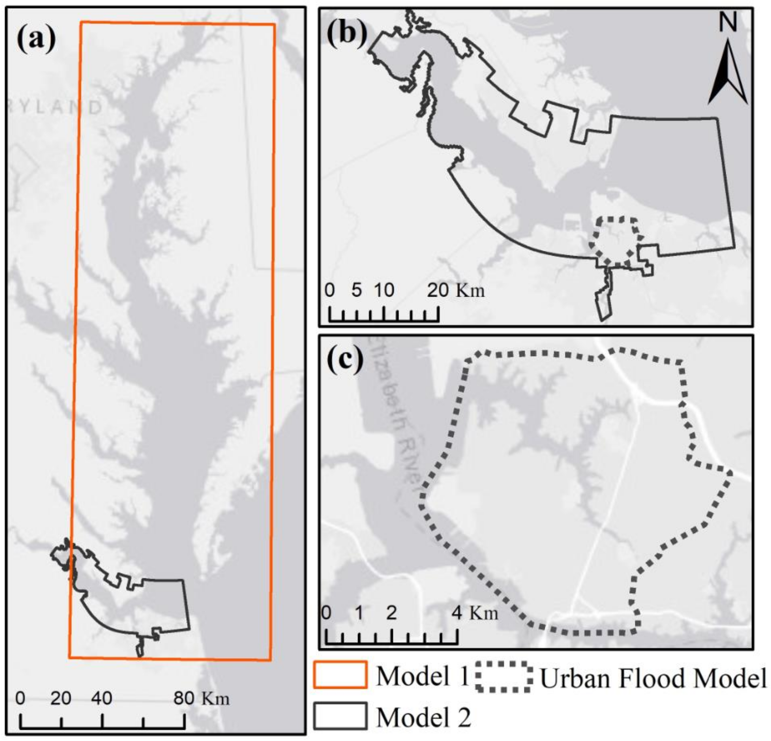
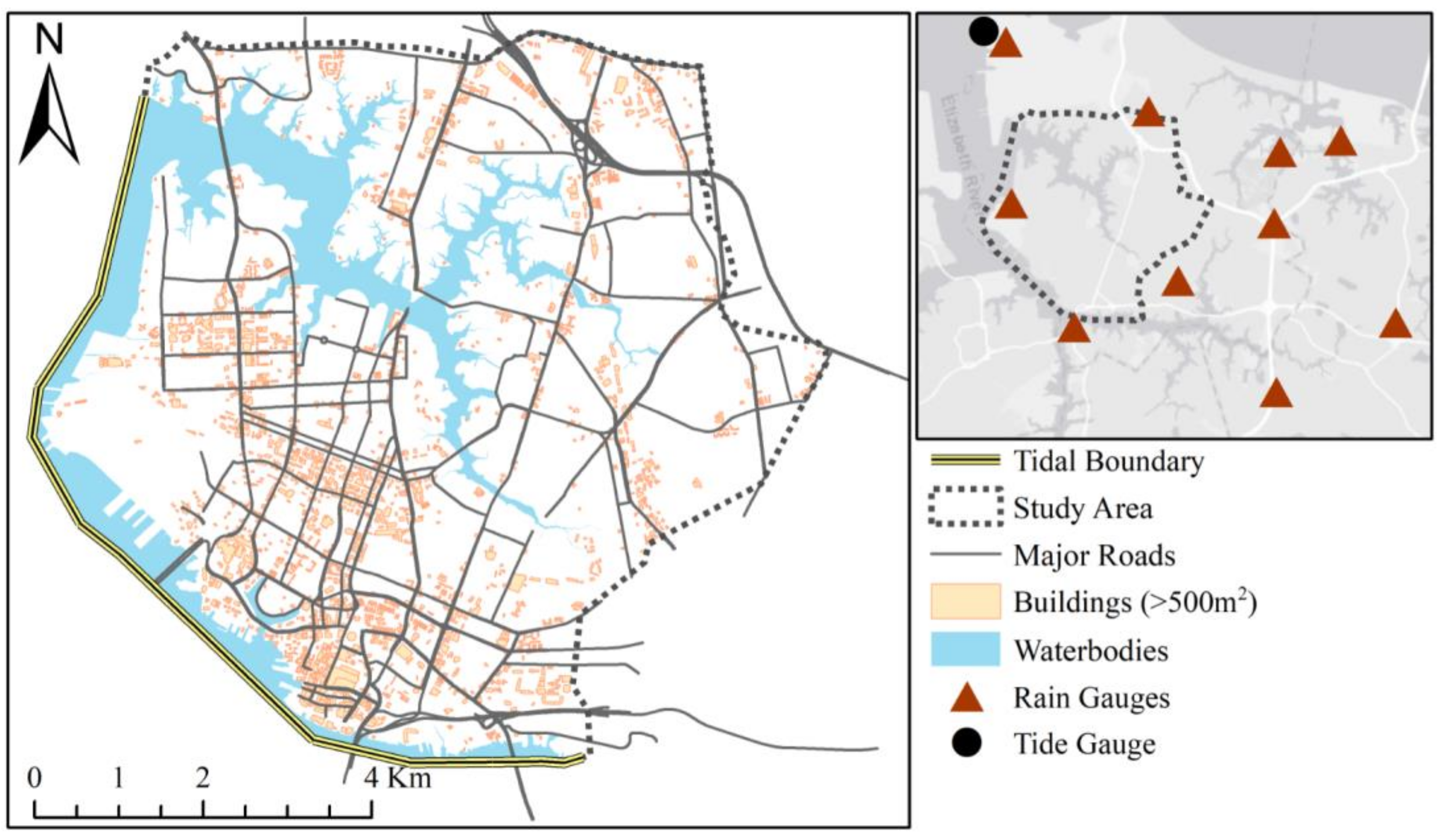
2.1. Study Area

The proposed methods are demonstrated in a portion of the City of Norfolk, Virginia, USA. Norfolk is in the heart of the Hampton Roads metropolitan area in southeast Virginia, and it is the home of the world’s largest naval base. This highly urbanized and low-lying city is located at the confluence of the James River, Elizabeth River, and Chesapeake Bay. Norfolk faces a series of natural hazard challenges, including flooding and other impacts of climate change, SLR, and subsidence [28,29]. This region is experiencing the highest rate of relative sea level rise (RSLR) on the US Atlantic Coast [28,30]. Studies have shown that flood frequency in this region has significantly increased due to SLR in the past decades, and this trend is expected to continue in coming decades [31,32,33]. Burgos et al. [32] indicates that nuisance flooding has increased 325% in Norfolk since 1960. More frequent major storm surge events have been observed in Norfolk over the past two decades and 17 major storm surge events have occurred in the past 85 years in Norfolk, but more than half of these events occurred in the past 15 years [34]. Meanwhile, because of climate change, the intensity of a 24-h duration rainfall with a greater than 1-year return period is expected to increase in Norfolk [35]. Studies have shown that rainfall intensity in Norfolk is projected to increase 30% to 40% by 2075 compared to 2000 levels under the high emission scenario [35].

2.2. Storm Surge Model

The coupled hydrodynamic and wave model developed by [20] was adopted to simulate storm tide under the current and future projected sea level conditions. The model is built on the Delft3D modeling suite (https://oss.deltares.nl/web/delft3d (accessed on 19 January 2018)). Because a storm surge is a shallow water process and the flow can be assumed well-mixed in the vertical direction, the model is applied in a 2D or depth-averaged mode with a single vertical layer.
Considering the computational cost of the storm surge simulation, models are normally designed to have a relatively coarser resolution at open sea and a higher resolution near shorelines, especially near critical regions. However, the computational efficiency is likely low when using a single grid crossing a large geographic region. Because the simulation time step is determined by the smallest cells in the grid, one approach to reduce the computational time is to set up the storm surge model in a nested structure. Tahvildari and Castrucci [20] nested the storm surge model at two levels, where low-resolution Model 1 covered most of the Chesapeake Bay, the Eastern Shore, and areas immediately offshore the Chesapeake Bay in the Atlantic Ocean, and the high-resolution Model 2 covered most of the urban areas at the south of the Chesapeake Bay. Model 1 used an equidistant grid with cell size 125 m × 200 m while Model 2 used a curvilinear grid with resolution of 10 m near critical infrastructures and 30–90 m away from these spots. Figure 1 shows the domains of the storm surge model and its location relative to the urban flood model introduced in the Section 2.3. During simulation, the velocity and water level estimates from Model 1 are transferred to Model 2 as boundary conditions.
The publicly available topography and bathymetry data from the National Oceanographic and Atmospheric Administration (NOAA) were used to build the model. The bathymetry and topography used in Models 1 and 2 were obtained from the Coastal Relief Model (CRM; 90 m horizontal resolution) and a regional dataset (10 m to 30 m horizontal resolution). The open boundary condition of Model 1 uses TPXO8 global tide model [36].

2.3. Urban Flood Model

The urban flood model that includes a 1D subsurface drainage network and a 2D surface domain was built for the southwest portion of Norfolk, as showed in Figure 2. The model domain has a total area of 56.4   km 2 , of which 8.7   km 2 . is open water. The study domain is a highly urbanized area with many artificial structures, including commercial and residential buildings, transportation networks, and stormwater infrastructure. The low-lying topography along with these structures create complex flow patterns and paths on both the land surface and in underground pipe networks. To accurately simulate street-level urban flooding, a 1D pipe/2D overland hydrodynamic flood model was built using the Two-dimensional Unsteady Flow (TUFLOW) model [37]. TUFLOW was adopted because it is capable of simulating both surface flow on a 2D domain and pipe flow via its 1D functionality along with a dynamic link between the two domains. TUFLOW is also capable of leveraging Graphical Processing Units (GPUs) in parallel, which can significantly speed up the model simulations. In [13], an urban flood model was built for the Hague Community located near downtown Norfolk. The spatial datasets, pipeline network, and parameter settings from [13] were adopted to build the urban flood model for the larger study domain in this study.
In this study, tide level observations were collected from the Sewells Point station (Station ID: 8638610) located along the northwest coast of Norfolk. The Sewells Point station, established in 1927, represents the longest tide record in Virginia. Rainfall observations were collected from two rain gauges maintained by the U.S. National Weather Service (NWS) and two rain gauges maintained by the Hampton Roads Sanitation District (HRSD). The locations of these gauges are shown in Figure 2.
The accuracy of topography representation is one of the most sensitive factors in the urban flood model. In this study, digital elevation model (DEM) representing the topography was built from a LiDAR-derived DEM dataset provided through the Virginia Geographic Information Network (VGIN) with 0.76 m × 0.76 m horizontal resolution [38]. This dataset, acquired in 2013, has a vertical accuracy of ±0.066 m. Buildings are another major factor describing the landscape in urban environments. Building footprint and height information were also gathered from VGIN. In the study domain, there are more than 29,000 commercial and residential buildings. To reduce the complexity and increase numerical stability of the model, only buildings with areas greater than 500   m 2 . were represented in the model. It was assumed that water will not enter the buildings, thus 3D building structures were added to the bare surface DEM.
The study domain has a complex drainage system. There are 9087 pipe sections with a total length of about 222 km. In this drainage system, more than half of the pipes were installed before 1950, and about 2000 pipes were installed before 1920. Given the age and complexity of the system, it is challenging for the city to survey the entire pipeline system and missing and inconsistent information may exist in the available surveyed data. We suspect this is a common challenge for other older cities as well. To reduce the complexity of the model, pipes with diameters smaller than 15 inches were excluded. Pipes inside buildings, underpasses, and tunnels were also excluded. Major pipes with missing information were retained, and it was assumed that their missing properties were consistent with their upstream and downstream pipes. For example, a pipe with a missing invert elevation is assumed to have the same bed slope as its upstream and downstream pipes. Then, the upstream and downstream invert elevations of the pipe are calculated by interpolating the inverse distance weighting (IDW). Smaller pipes with missing information were excluded from the model. After these data cleaning steps, 6213 pipe sections were retained with the total length of about 179 km.
TUFLOW solves the full 2D depth averaged momentum and continuity equations for shallow water free surface flow and incorporates the full functionality of the ESTRY one-dimensional (1D) hydrodynamic network model [37]. The same technique and parameter settings for coupling the 2D land surface domain and the 1D pipe network used by [13] were adopted by the current study. Please reference [13] for details. The study domain has an average imperviousness ratio of 41% and a shallow groundwater level, which can reach the surface during storm events that cause flooding. Thus, infiltration is expected to not have a significant influence on significant flood events, and therefore, it was not parameterized in the urban flood model. This presumes saturated conditions for the non-impervious surfaces in the urbanized watershed at the start of the model simulation period. Lastly, a detailed simulation of bridges, underpasses, and tunnels were excluded in the model to focus on other regions within the study domain. Future work can add additional complexity to the model to include these additional processes and features of the landscape.

2.4. Model Coupling

The storm surge model and the urban flood model were linked through the tidal boundary portion of the study domain, as shown in Figure 2. The total length of the tidal boundary is 12.5 km. The tidal boundary was split into nine sections approximately parallel to the regional coastlines with no sharp change in orientation. The length of these sections varies from 950 m to 2000 m. In a simulation, the storm surge model was executed first, separately from the urban flood model. Then, time series of tide level from the simulation were extracted and averaged across each section in the flood model using an automatic post-processing procedure. This step prepared the boundary condition of water stage versus time for each tidal boundary section. In the urban flood model, the initial tide level was set as the averaged low tide level in the past four decades, which is about −0.9 m (NAVD88) at Sewells Point station. Then, the tide level boundary conditions and rainfall inputs were fed into the urban flood model to generate high-resolution flood simulations.
The simulated tide flow velocity from the storm surge model was not used by the urban flood model because of the inability to specify velocity boundary conditions in the version of TUFLOW used in this study. This simplification may cause underestimation of direct storm tide inundation, but we do not suspect this underestimation to be significant. Nonetheless, in an effort to compensate for potential underestimation, a post-processing procedure was applied to modify the inundation extent for each time step and the maximum inundation maps. First, simulations from the storm surge model were extracted within the urban flood model domain. Second, these storm surge simulations were resampled to the mesh of the urban flood model. Third, these resampled storm surge simulations were compared with the urban flood model simulations in each cell, and the maximum values were selected as the final result. This procedure was then repeated for each simulation time step. The procedure resulted in the combined results that can be thought of as the worst-case situation from the two models, which are valuable for flood hazard mitigation purposes.

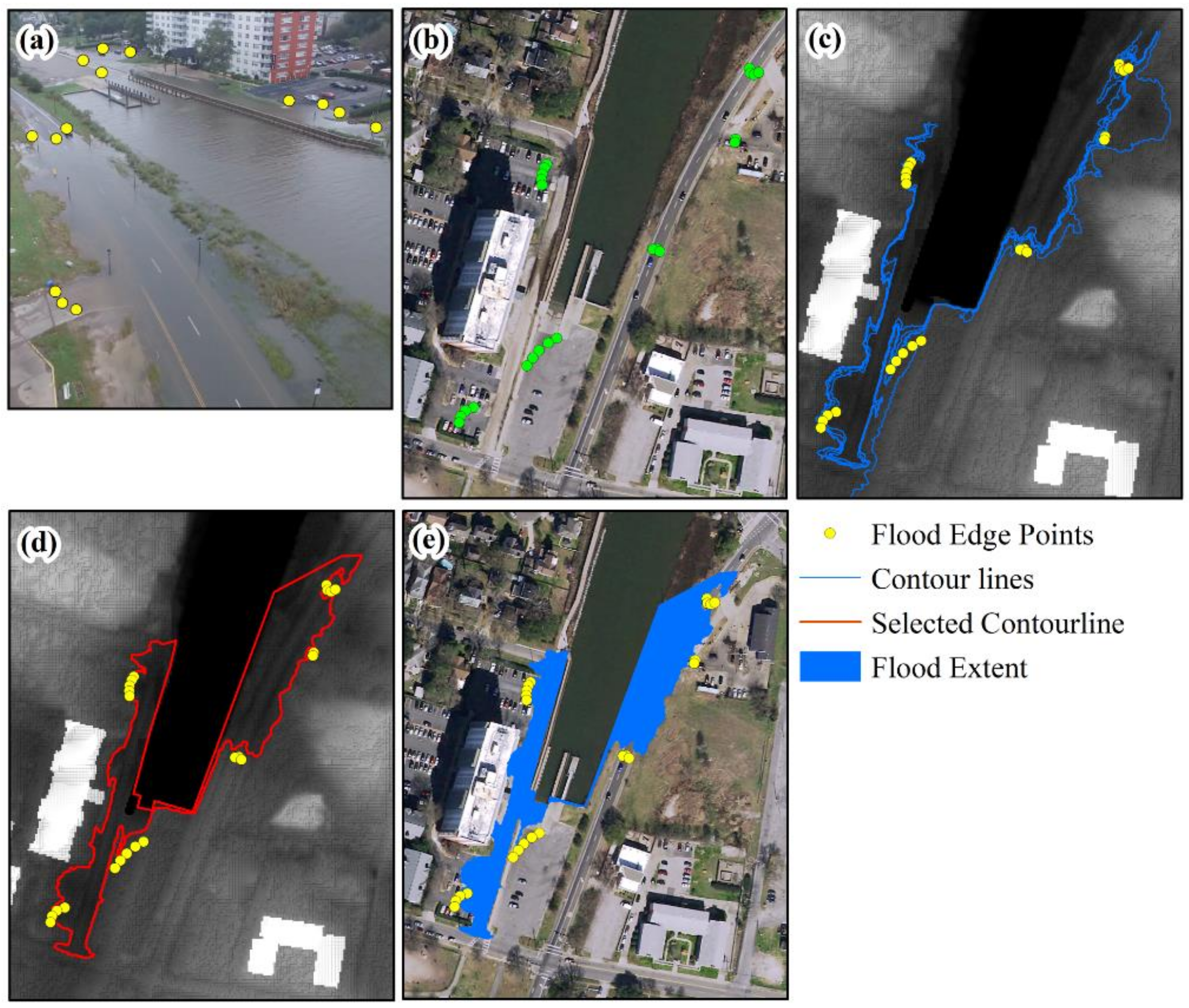
2.5. Model Evaluation

Direct flood observations in urban areas are rare; however, they are essential for urban flood model evaluation and calibration [39]. A USGS gauge (latitude: 36.8588°, longitude: −76.2986°) was installed in the Hague Community near downtown Norfolk during Hurricane Irene (2011). Records from this gauge were used to assess the model performance at that location near the shoreline.
Spatially distributed flood observations, for example flood extent, have unique values for evaluating the performance of 2D models. Crowdsourced data, such as photos or camera footage of flooded areas, newspaper reports, personal interviews, and flooding information shared by users on social media, can be converted to inundation information ([39,40,41,42]). The inundation information is valuable for evaluating 2D urban flood models. In this study, imagery data were adopted as an additional innovative data source to evaluate the coupled flood model. On 10 October 2016, the day after the peak of Hurricane Matthew in Norfolk, drone footage was captured by the Norfolk Department of Emergency Management and is available online (https://www.youtube.com/watch?v=R8ZYxubUo-w (accessed on 23 May 2019)). In the drone footage, three scenes were captured inside the current study domain. Because the flight information, such as flight height, orientation, camera angle, and precise geolocation, is missing from the record, the footage cannot be directly georeferenced. Therefore, we created a method to extract flood extent by manual flood edge identification and GIS processing.
As a demonstration, Figure 3 shows the procedure of the proposed method for extracting flood extent. The first step was to identify flood edges from multiple frames captured in the same scene. For example, in Figure 3a, the flood edge intersected with several features in the surrounding area, such as streetlamps, street curbs, and parking space lines. Flood edge points close to these features were manually selected and geolocated (Figure 3b). The following step was to generate elevation contour lines crossing each flood edge points by using the high-resolution LiDAR dataset (Figure 3c). The next step was to separately calculate the total distance of each contour line to all flood edge points. Among all the contour lines, the one with the minimum total distance was selected as the inundation edge (Figure 3d). Finally, the areas lower than the contour line elevation were assumed to be flooded at that time. Using the same procedure, the flood extents in all three scenes were extracted. One assumption of the procedure was that the water surface is level or nearly level, which is plausible for this case because the footages were captured one day after the storm peak.

2.6. Combined Storm Scenarios

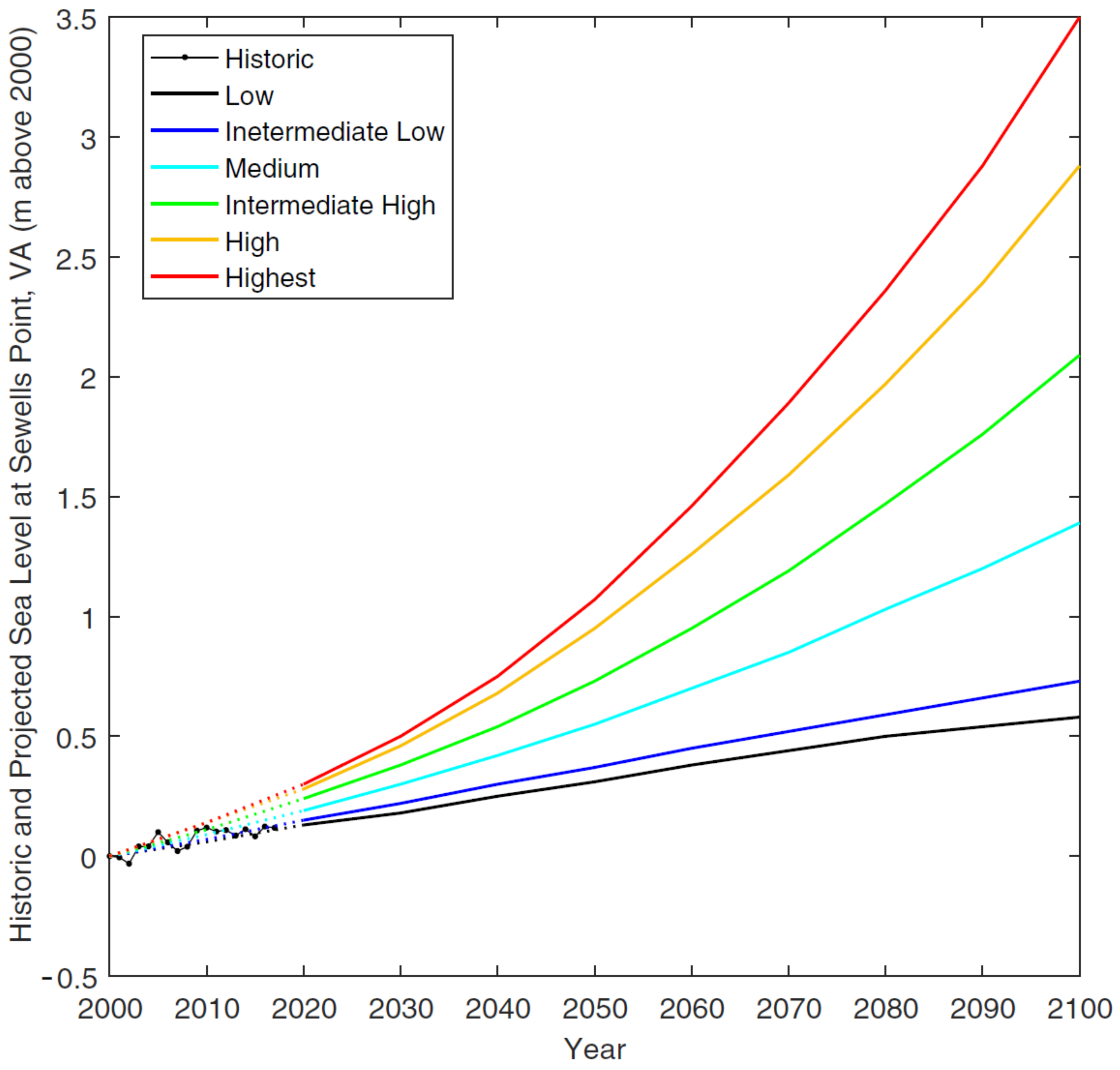
2.6.1. Relative Sea Level Rise Scenarios

Virginia’s coast is a hot spot of RSLR due to climatic and non-climatic (e.g., subsidence) processes. The primary non-climatic component is vertical land movement (VLM; subsidence or uplift), but it also includes sea surface height changes associated with glacial isostatic adjustment [29]. In this study, the RSLR scenarios were obtained from [29]. RSLR is equal to the sum of global mean sea level (GMSL) change and local relative sea level (RSL) change as follows:
R S L R x , t = Δ G M S L t + Δ R S L x , t
where R S L R x , t is the total RSLR estimated for spatial location x and time t, Δ G M S L t is the GMSL rise at time t, and Δ R S L x , t is the total RSL change relative to RSL at the reference time (t0). From [28], the RSL change that occurs in each GMSL rise scenario consists of contributions from climate-related processes and non-climatic background RSL changes. The total RSL change is defined as
Δ R S L x , t = C l i m a t i c   Δ R S L x , t + B a c k g r o u n d   R S L   R a t e x t t 0
where Climatic Δ R S L x , t is the RSL change affected by climate-related processes at spatial location x and time t, and B a c k g r o u n d   R S L   R a t e x is the non-climatic component of RSL change, which is assumed to be linear in time.
We adopted the RSLR scenarios from [29], which revised the upper and lower bounds of SLR scenarios from the most up-to-date scientific literature. Sweet et al. [29] recommends six GMSL rise scenarios from 0.3 m to 2.5 m by the year 2100. These six GMSL rise scenarios are Low, Intermediate-Low, Intermediate, Intermediate-High, High, and Extreme, which correspond to GMSL rises of 0.3 m, 0.5 m, 1.0 m, 1.5 m, 2.0 m, and 2.5 m, respectively. Based on [29], Tahvildari and Castrucci [20] calculated the RSLR scenarios at the Sewells Point tide gauge with the mean background RSL rate of 2.47 mm/y. In this study, we adopted these RSLR projections, as shown in Figure 4. Note that these RSLR projections are referenced to zero at 2000.
In this study, 10 and 50-year storm surge events, based on water level observation at the Sewells Point tide gauge, were chosen to represent a moderate and a high storm surge, respectively. The storm surge elevations for the 10-year (1.55 m NAVD88) and 50-year (2.07 m NAVD88) recurrence intervals were obtained from the FEMA Flood Insurance Study for Norfolk [43]. The strongest hurricane that affected the region in the past century was the Chesapeake–Potomac hurricane (1.95 m NAVD 88 at peak) in 1933, which caused a storm surge slightly lower than a 50-year water level. The peak of Hurricane Irene (1.81 m, 2011) falled between the 10-year and 50-year tide levels under the current climate condition. The track and central pressure information of Hurricane Irene (2011), obtained from the NOAA National Hurricane Center [44], were used to generate the pressure and wind field over the storm surge domain. Then, the wind intensity was adjusted to produce the 10 and 50-year water levels. For further details, please refer to [20]. We selected the high RSLR scenarios The track and central pressure information for a conservative scenario. The high GMSL rise projection corresponds to a 2.0 m rise by 2100 with the probability of exceedance at 0.1% (RCP2.6) and 0.3% (RCP8.5). We selected 2070 as the targeted year to compare with the current climate condition. Table 1 summarizes the storm surge and RSLR scenarios investigated in this study. Note that the current climate condition refers to water level and climate conditions in year 2020.

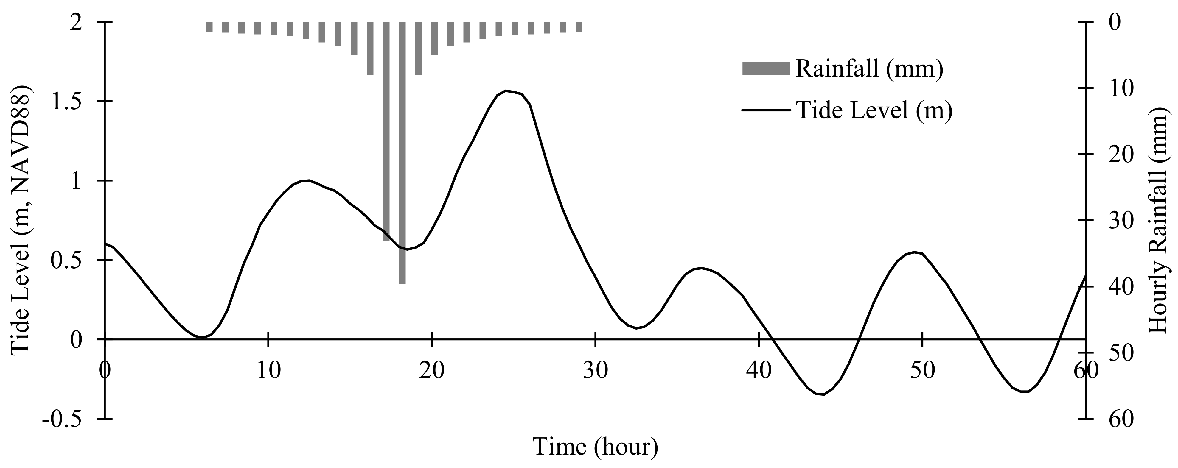
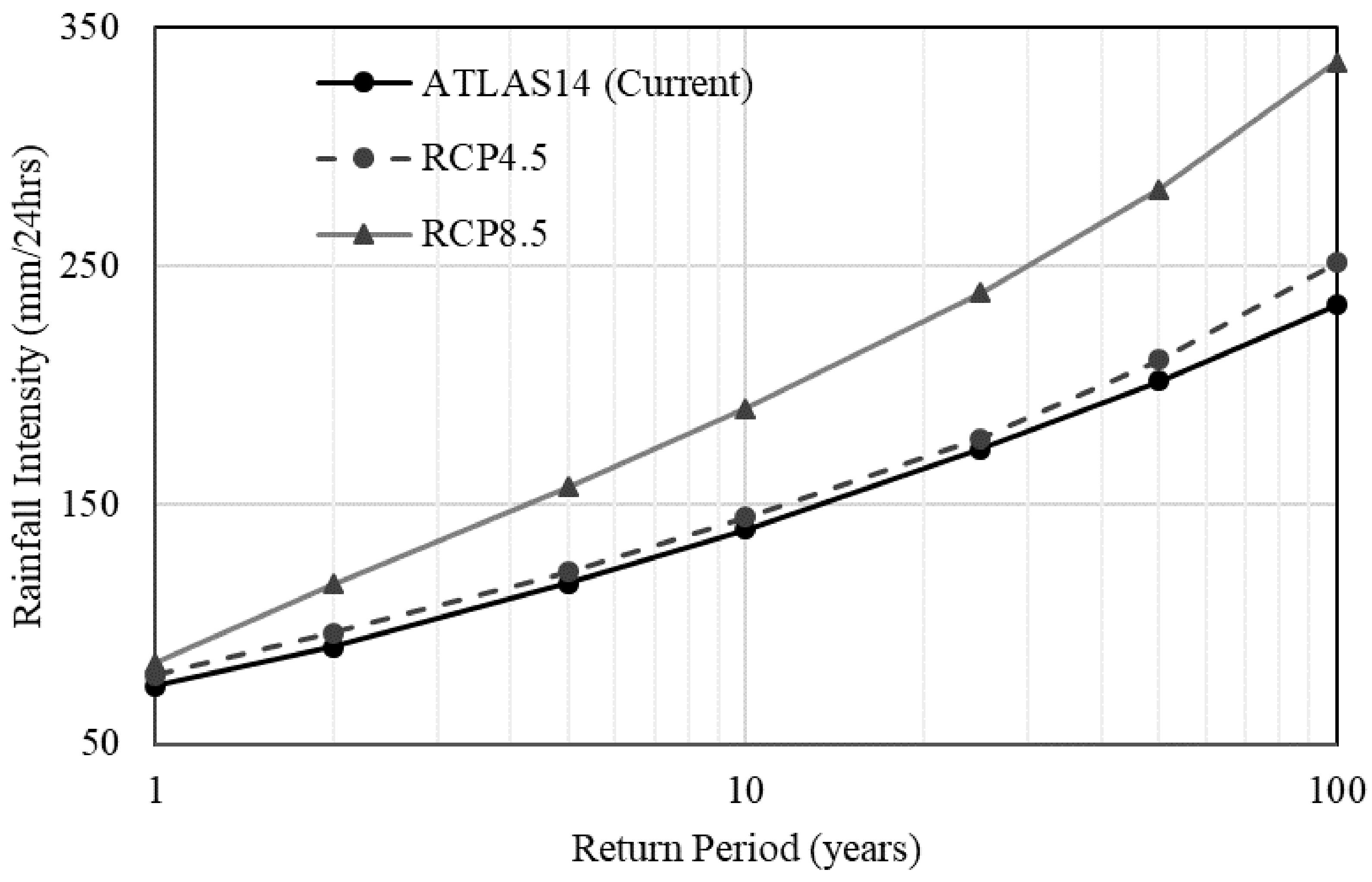
2.6.2. Rainfall under Climate Change Scenarios

The impact from the change in rainfall intensity due to climate change is demonstrated by one climate change scenario. Changes in rainfall intensity are one of the primary impacts of climate change in urban areas [45]. Changes in other factors, for example, temperature and wind speed, were not simulated in this study. Following the example of [35], the changes in rainfall intensity in Virginia were estimated under multiple climate change scenarios. Generally, the future rainfall frequency for the study area was estimated by analyzing future rainfall projections. Then, rainfall scenarios were generated based on rainfall frequency and assumed rainfall distribution.
Rainfall projections from global climate models (GCMs) or regional climate models (RCMs) are commonly used to estimate the impacts of climate change. The spatial resolutions of GCMs are generally coarse, i.e., greater than 100 km [45]. The spatial resolutions of RCMs are typically in between 12 km to 50 km [22,45]. In this study, the rainfall projections were collected from the Coordinated Regional Climate Downscaling Experiment [46], which is a global repository of RCM simulations covering all continents of the globe. In CORDEX, climate projections are downscaled using dynamic RCMs for 14 domains with the IPCC 5th GCMs outputs as the boundary condition. The CORDEX products in North America are available for the Representation Concentration Pathway (RCP) 4.5 and RCP 8.5 climate scenarios. The spatial resolutions of these products vary from 22 km to 44 km. In the current study, the daily rainfall projections for the period of 1950 to 2100 were extracted at the Norfolk International Airport. Then, the rainfall projections were bias corrected using historical observations from 1950 to 2005 by using the modified Empirical Quantile Mapping (EQM) method proposed by Themeßl et al. (2011). In the EQM method, the historical observation and hindcast simulation from 1950 to 2005 were used to build a quantile–quantile mappings (QQMs). Next, the QQMs were applied to correct the bias in the precipitation projections.
The bias corrected rainfall projections were then used to estimate rainfall frequency. Because future rainfall is non-stationary under a changing climate, rainfall frequency is not fixed. However, an assumption in this study was that rainfall frequency is fixed for the periods of interest, for example, from 2056 to 2085. The same statistical methods and probability distribution, Generalized Extreme Value (GEV), used to construct the NOAA Atlas 14 IDF curves [47], were chosen to construct the rainfall frequency used in this study. Shen et al. [13] summarized and analyzed the rainfall durations of large storm events observed at the Norfolk International Airport. This study found that the majority of these large storms had rainfall durations of about 24 h. Thus, the current study focused on the 24-h rainfall event to represent large storm events. The rainfall intensities for a 24-h duration storm event with return periods varying from 1 to 100 years were estimated under RCP4.5 and RCP8.5 scenarios for the period 2056–2085 (simply stated as the 2070 Rainfall Frequency in the remainder of this paper). Figure 5 shows the comparison between the 2070 rainfall frequency and the current rainfall frequency obtained from NOAA Atlas 14 (https://hdsc.nws.noaa.gov/hdsc/pfds/pfds_map_cont.html (accessed on 10 May 2019)).
According to Merkel et al. [48], the study domain is located in the region of NOAA Type-C rainfall distribution zone. Therefore, we adopted the NOAA Type-C rainfall distribution for creating synthetic rainfall hyetographs for the 24-h rainfall scenarios. We used the 10-year and 50-year rainfall scenarios to model flooding because they represent significant, but not catastrophic, flood impacts to the study area. We chose the RCP8.5 scenarios to demonstrate the potential impact of these more significant climate change scenarios on flooding.
To explore the combined impact of rainfall and storm tide under both the current climate condition and selected future climate scenarios, the designed storm tide and rainfall scenarios were combined into a series of storms for the coupled flood model. Shen et al. [13] investigated the time lag between storm surge and rainfall and showed how it would significantly influence the impact of flooding in the study region. Different time lags were not explored in this study. Instead, the time lag was set to be the same as what was observed for Hurricane Irene (2011) where the rainfall peak was 8 h ahead of the tide level peak. An example model inputs for a 10-year rainfall and a 10-year storm surge event in 2020 is provided in Figure A1 of Appendix A.

2.7. Assessing Transportation Impacts

Flood simulations outputs were used to estimate impacts on the transportation network within the study area. In this study, the impact on roads is described as road closures and the criterion for closing a road was assumed to be a flood depth of 0.3 m or more on the roadway, as predicted by the flood model. This flood depth is a conservative road closure criterion because it is the height of the air inlets of most vehicles [17].
The transportation network was obtained from the City of Norfolk (https://www.norfolk.gov/1596/Geographic-Information-Systems (accessed on 15 July 2019) and the traffic data of major roads were gathered from the Virginia Department of Transportation (VDOT: https://www.virginiadot.org/info/ct-TrafficCounts.asp (accessed on 15 July 2019). The study domain contains 6983 road links and 450 major road links, as shown in Figure 6. The annual average daily traffic (AADT) of the major roads varies from 60 to 151,000. About 60% of the major road links AADTs are greater than 10,000.

3. Results and Discussion

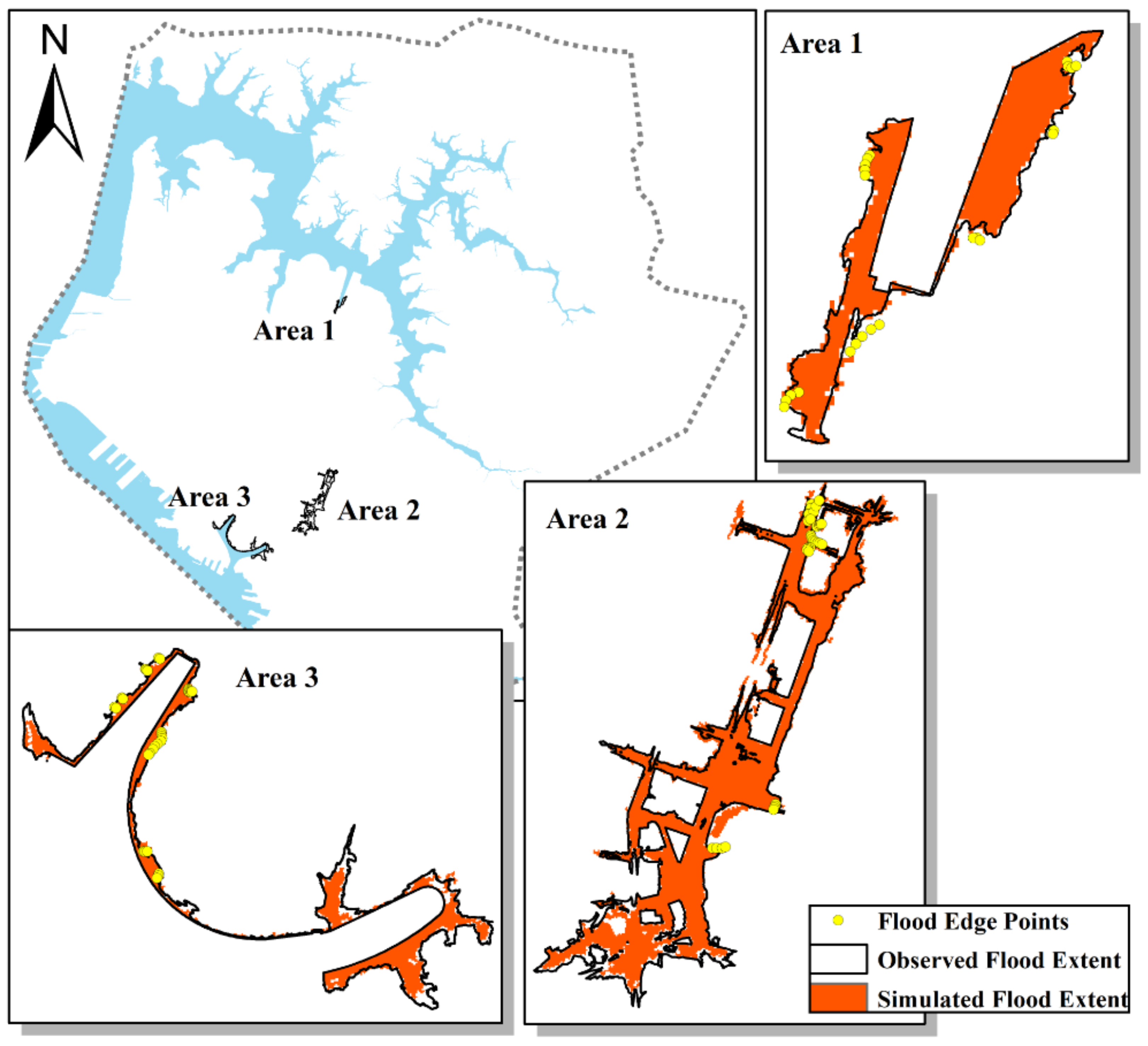
3.1. Model Evaluation

The storm surge model was built to assess the impact of sea level rise in Norfolk. The storm surge model was validated at two NOAA gauges (Chesapeake Bay Bridge and Tunnel and the Sewells Point tide gauge) during Hurricane Irene (2011) in [20]. The comparison showed a good match between the storm surge simulation and observations with a root-mean-square-error (RMSE) equal to 0.137 m and 0.138 m at these two gauges, respectively [20]. For detailed information about the storm surge model validation, please refer to the study [20]. Here we focus on evaluating the performance of the coupled flood model, rather than just the storm surge or urban flood model in isolation.
A USGS gauge (latitude: 36.8588, longitude: −76.2986) was temporarily deployed in the Hague Community for the Hurricane Irene (2011) storm event at the location shown in Figure 7a. A comparison between the water level observations at this USGS gauge and the output from the coupled model is provided in Figure 7b. Overall, the simulation showed a close match with the observation in both phase position and magnitude. The coupled model slightly underestimated the peak water level (by 0.02 m) and had a positive phase shift (of about 30 min) compared to observations. Given that this study focused more on the peak flood impact than the timing of these impacts, these results were deemed acceptable based on this evaluation.
Given that 2D flood models provide flood inundation map outputs, we also evaluated the flood model using areal imagery data. As shown in Figure 8, flood extents were extracted from drone footage at three locations inside the study domain for the Hurricane Matthew flood event, as described in the Section 2. Area 1 is directly connected to the tidally influenced Lafayette River, and flooding is therefore controlled by the downstream tidal boundary condition. Area 2 is about 700 m away from the shoreline and is under the combined impact of tidal flooding and pluvial flooding, as shown in [13]. Area 3 is located at the shoreline and exposed to direct tidal flooding. Therefore, even though flood extents are available only at three local regions, they represent areas where tidal, pluvial, or tidal and pluvial flooding are at play and can serve as valuable evaluations of the overall model system.
Precision, recall, and F1-score [49] were adopted as accuracy metrics to evaluate the performance of the coupled flood model. Precision and recall are commonly used metrics to compare the relevance between model predictions and ground truth for image classification. Recall represents the proportion of flood extent that was correctly identified by the model compared to the ground truth flood extent, taken from the imagery, and is defined as
Recall = True   flood   extent   simulation Total   true   flood   extent
Precision represents the proportion of flood extent that was correctly identified by the model compared to the total flood extent produced by the model, and is defined as
Precision = True   flood   extent   simulation Total   flood   extent   simulation
The flood extent precision, recall, and F1-score in each evaluation area are summarized in Table 2. Based on Figure 8 and Table 2, the spatial distribution of the simulated flood extents match well with the flood extents extracted from the drone images. The overall F1-scores across these three areas vary from 0.68 to 0.88. Within these three areas, the model shows the best performance in Area 1 with a precision and recall of 0.92 and 0.84, respectively. In Area 2, the topography and mechanisms of flooding are more complex than in the other two areas. Figure 8 illustrates that most of the underestimated flood extent in Area 2 was in the southwest of that area, which includes the parking lot of the Virginia Opera and intersections of three major roads. The model shows the lowest precision and recall in Area 3, which faces direct tidal flooding. The underestimation is most pronounced in the eastern portion of Area 3. There is no direct observation or footage available for this portion of the study region, so the flood extent had to be estimated from GIS analysis using digital terrain data. Further investigation is needed to better understand flooding in this area and whether the model is underestimating flooding in this region. Despite these challenges and opportunities for improvement, the model shows good performance overall across the three evaluation areas as judged by precision, recall, and F1-score.

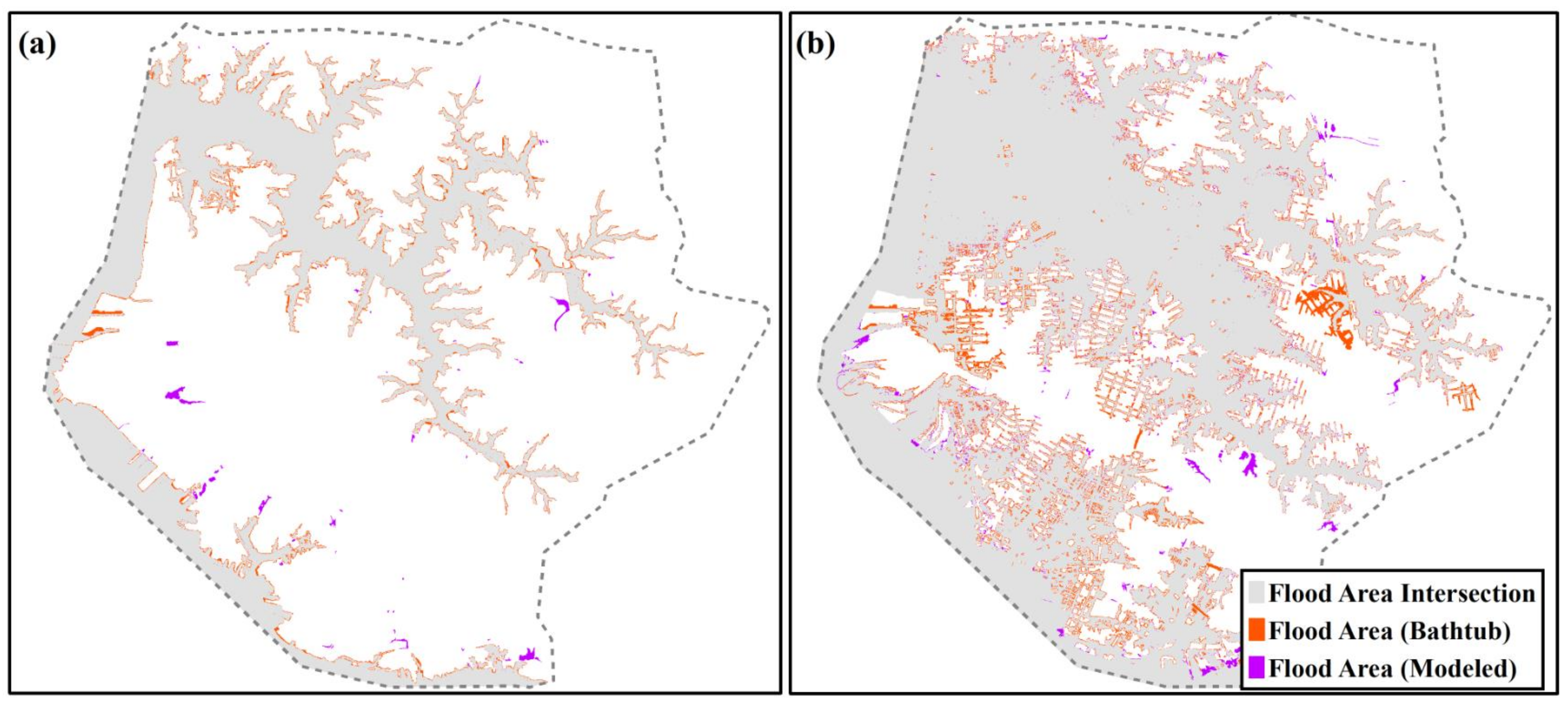
3.2. Comparison with the Bathtub Method
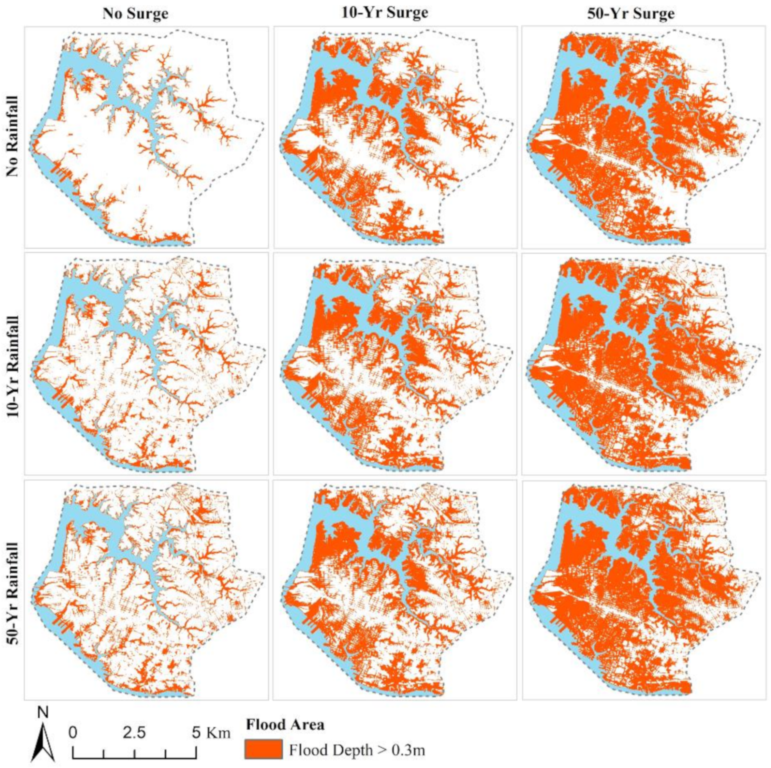
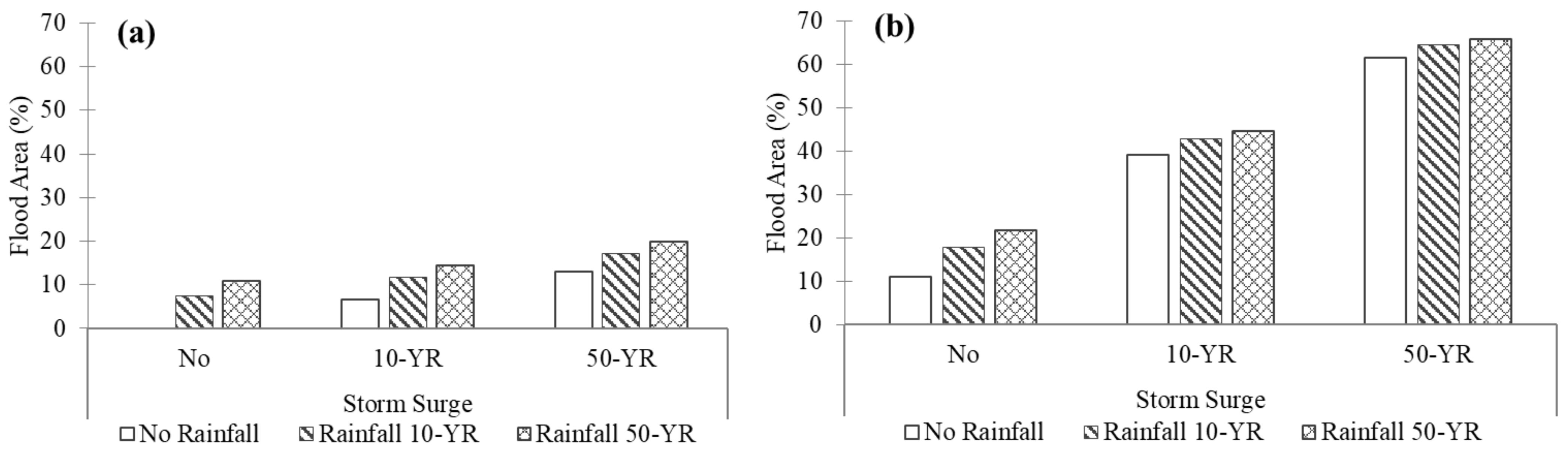
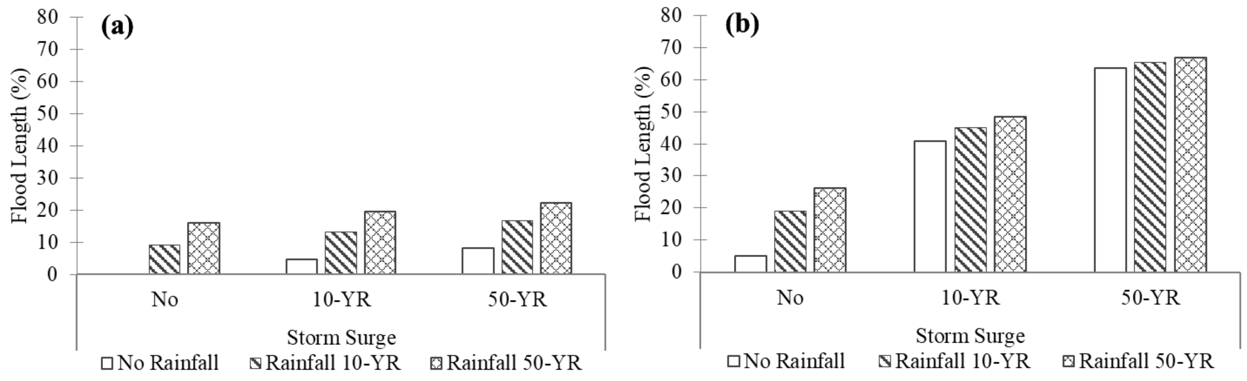
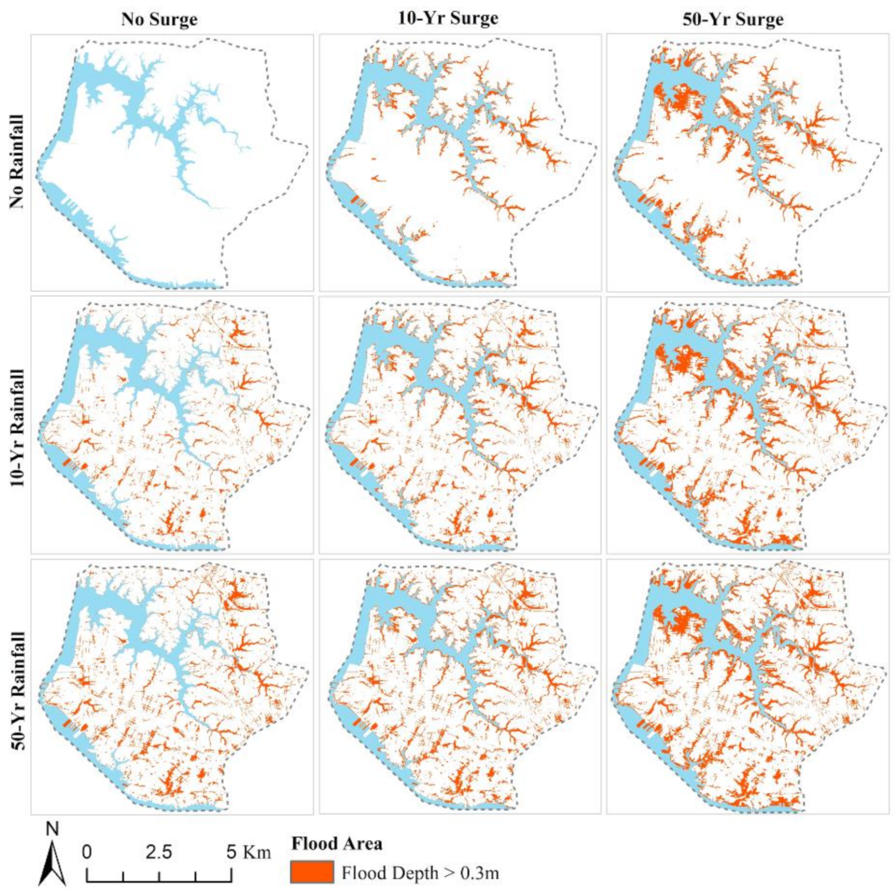
This section presents results of the comparison between the coupled flood model and the bathtub method for assessing the impact of SLR and storm tide in coastal regions. Results from the 10-year storm tide events in current (2020) and future (2070) sea level conditions were taken as a demonstration (Figure 9). Similar to results shown by [27], we found that the bathtub method estimated greater flood extent for regions topographically and hydraulically connected to open water. The flood extent comparison is qualified by the following function.
Diff = Flood   Area bathtub Flood   Area modeled Flood   Area bathtub × 100 %
In Figure 9, the bathtub method estimated greater flood extent near the shoreline by 9.5% and 3.1% in 2020 and 2070, respectively. However, due to the existence of underground drainage systems in the coupled flood model, several inland local depression areas were simulated by the model to be flooded by backward pipe flow from high tide level but not by the bathtub method. Compared to the bathtub method, the flood model estimated 9.0% and 4.0% more flood extent in the inland region in 2020 and 2070, respectively. This is because the bathtub method does not account for rainfall-driven flooding, which in combination with the backwater pipe flow, is responsible for this inland flooding.
The coupled flood model and bathtub method were also compared for other storm tide scenarios under the 2020 and 2070 sea level conditions. From Figure 10, we can draw the following insights. First, the greater flood extent estimation of the bathtub method increases as the storm return period increases. Second, when the tide peak level is lower than a certain level, for example in the “no storm surge” 2070 scenario in Figure 10, the total flood area from the coupled flood model can be greater than the bathtub method.

3.3. Flood Areas

The flood maps for all combined storm events under both the 2020 and 2070 climate conditions are presented in Figure 11 and Figure 12. As expected, tidal flooding primarily occurs near coastline and tidal rivers with low-lying topography. In Figure 11, under the no rainfall condition, several inland areas are flooded by the 10-year and 50-year storm tide. Flooding in the local depression areas seems to be caused by backward pipe flow because these stormwater pipelines in this region lack a tide gate or flap gate to prevent backward flow. Figure 11 shows how pluvial flooding is distributed across the inland region, specifically gathering in areas that lack effective drainage infrastructure. In the analyzed rainfall scenarios from Figure 12, the flood extents are estimated to increase dramatically due to the increase of rainfall intensity and SLR in 2070. Under the no storm surge condition in 2070, a large portion of the coastline region is estimated to be flooded due to the increase of the base tide level alone. When affected by storm tide on top of SLR, the majority portion of the study domain is expected to be flooded.
Figure 13 shows the percentage of the total flooded area for all analyzed combined storm scenarios. Under the 2020 condition, the combined storm events are estimated to flood 7% to 20% of the land area, depending on the storms return period. Under the projected 2070 conditions, the combined storms would flood 18% to 66% of the land area under these same return period storms. From Figure 13a,b, the so called “sunny-day flood” scenario (just high tide with no rainfall or storm tide) in 2070 is still estimated to flood 11% of the land area. This flood extent is nearly equivalent to a 50-year (13%) storm tide in 2020. From 2020 to 2070, the flood extent increase by about 11% on average for both the 10-year and 50-year rainfall scenarios under the no storm tide condition. That increase is primarily caused by the combined effect of rainfall intensity increases and RSLR, causing backwater pipeline flooding and a reduced pipeline capacity. Over the same time span, even with no rainfall and only storm tide, the flooded extent increase by 32% and 49% for the 10-year and 50-year storm tides compared to the no storm surge scenario, respectively. Taking the 50-year storm tide in 2070 as an example, storm tide alone will flood 62% of the land area. Combined with a 50-year rainfall event, the storm tide is estimated to flood 66% of the land area, which means that only 4% of the total flooding in this scenario is attributed to rainfall. Therefore, tidal flooding has a greater impact on flooding compared to pluvial flooding in the study domain, under projected RSLR scenarios.

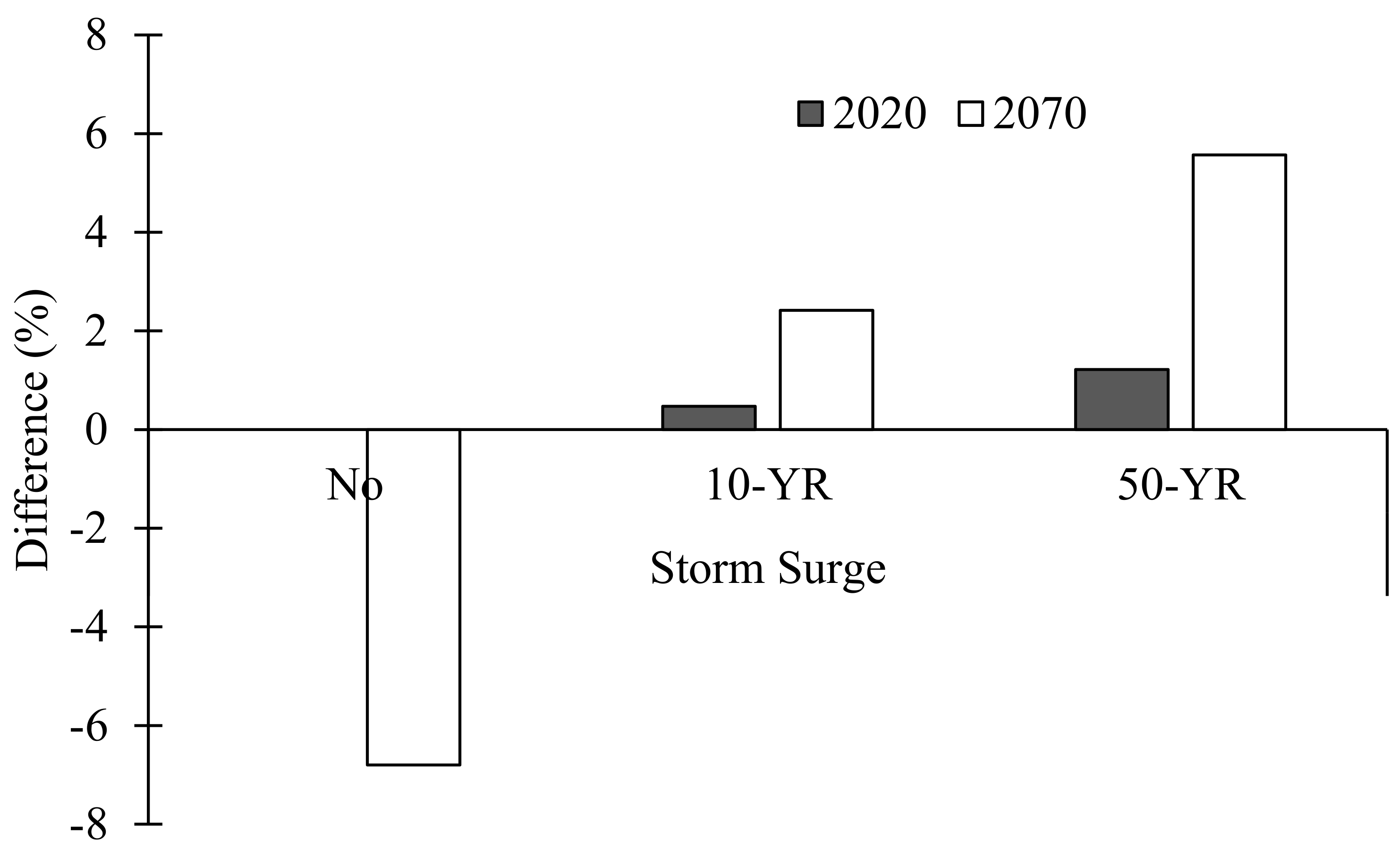
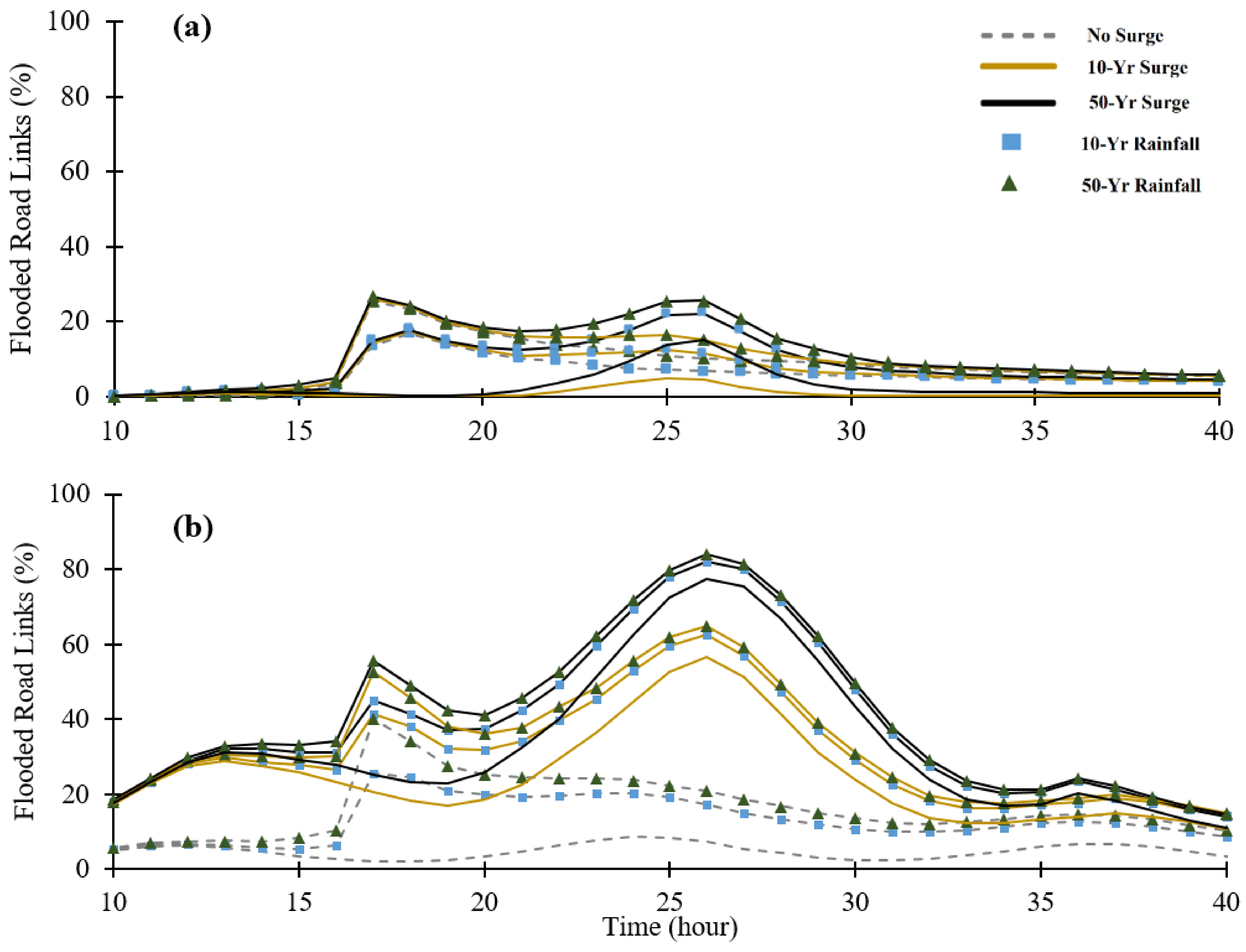
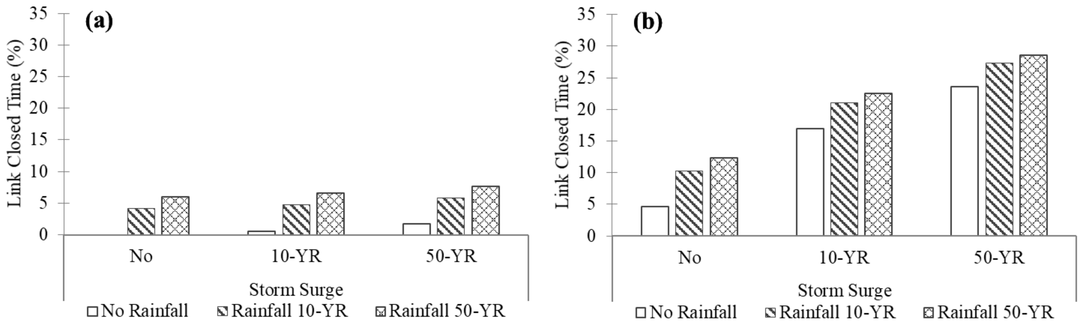
3.4. Flood Impact on the Transportation Network

The coupled flood model provides a method for estimating flood impact on critical urban infrastructure systems. As a demonstration, the flood model was applied to assess the flood impact to transportation networks under a set of storm scenarios.
The impact to the transportation network was quantified as a percentage of flooded road length to total road length in the study region (Figure 14). Under 2020 conditions, the analyzed storm events would flood between 4.6% (10-year storm surge alone) to 22.3% (50-year storm surge and 50-year rainfall) of roadways. In 2070, the flooded roadways are estimated to vary from 19.0% (10-year rainfall alone) to 66.9% (50-year storm surge and 50-year rainfall). Meanwhile, in a sunny day scenario (high tide alone with no rainfall or storm surge) in 2070, 5.2% of the road length would be flooded. This sunny day or nuisance flooding projected for 2070 is similar to the impacts of a 10-year storm tide in 2020.
One major advantage of a dynamic flood model, compared to static methods such as the Bathtub method, is its ability to simulate the duration of flooding rather than just the peak flooding impacts. Figure 15 shows the percentage of roadway links flooding during the storm scenarios. The rainfall peak is 8 h ahead of the tide level peak in these scenarios, as explained in the Section 2, resulting in two peaks for roadway flooding impacts. Under 2020 conditions (Figure 15a), storms with both significant rainfall and storm tide result in similar impacts during the starting (rainfall dominate) and ending (storm tide dominate) portions of the storm event. However, under 2070 conditions (Figure 15b), the storm tide becomes a more impactful flooding mechanism. In this scenario, a storm with both significant rainfall and storm tide would suffer the most impact during the portion of the storm where storm tide was the dominant flooding mechanism. Looking at the impact from storm scenarios with only rainfall-driven flooding, the maximum number of flooded road links is projected to increase by 8.7% and 14.8% under the impact of 10-year and 50-year rainfall events, respectively, from 2020 to 2070. For a tidal-driven flooding scenario with no rainfall, the maximum percentage of flooded road links will increase by 51.7% and 62.4% for 10-year and 50-year storm tide events, respectively. This suggests the impact of flooding on the transportation network will be most affected by tidal-driven flooding compared to rainfall-driven flooding under the projected RLSR and climate change scenarios.
To summarize the spatial-temporal impact on the transportation network, a metric named the total link closed time (TLCT), is introduced. TLCT is defined as
T L C T = i N T c l o s e d ,   i T t o t a l × N × 100 %
where, N is the total number of road links, T c l o s e d ,   i is the total closed (due to flooding) time of link i during a storm event, and T t o t a l is the total length of the simulation period. The TLCT for the road links in the study domain was computed for all storm scenarios, and the results are shown in Figure 16. The TLCT is sensitive to the increase of both rainfall intensity and storm surge under the 2020 conditions, as illustrated in Figure 16a. Under these conditions, a 10-year rainfall would result in a TLCT of 4.2%, but a 50-year storm surge would cause a TLCT of only 1.8%. This is because the duration of pluvial flooding is longer than tidal flooding in the study region under current conditions. However, these conditions are expected to change by 2070. As shown in Figure 16b, the 10-year and 50-year storm tide events will result in TLCTs of 16.9% and 23.6%, respectively. Interestingly, adding the impact of rainfall to these scenarios increases the TLCT by only 1.3% to 4.1%. Therefore, storm tide events are expected to be the dominant factor interrupting the transportation network in 2070. Finally, sunny day or nuisance flooding is expected to cause a TLCT of 4.6%, which is more than two times that of a 50-year storm surge in 2020. Considering the duration of flooding and its impact on transportation systems, nuisance flooding in 2070 is likely to be a serious challenge for transportation management unless efforts are made to prevent tidal flooding impacts, such as preventing the backflow of tidal water through subsurface drainage networks.

4. Conclusions

The overarching objective of this study is to advance methods for assessing the combined impact of rainfall and storm tide on coastal cities under selected future climate scenarios. As an example application of the methodology, a coupled flood model consisting of a 1D stormwater pipe/2D overland flood model and a 2D storm surge model was built for a large portion of Norfolk, VA. The coupled flood model can simulate the hydrodynamic and wave processes of a storm tide in the ocean and its progression on land, as well as pluvial flooding due to excess rainfall and resulting runoff. Simulating the complex stormwater drainage infrastructure system in the model makes the coupled flood model especially suited to analyzing flooding in an urban environment. This detailed numerical model can generate simulations with high spatial-temporal resolution to support flood hazard assessment and management. We made use of available point observations and imagery data to evaluate the model performance and created an approach to extract flood extent from drone imagery to evaluate the model. The model was compared to the more commonly used bathtub method for flood hazard assessment and the utility of the model is demonstrated by quantifying flooding impacts on the transportation network within the region.
Both the storm surge model and the overland flood model were built using hydrodynamic models, which are known to have significant computational demands [50]. Given the practical limitations imposed by simulation runtime, the number of climate change and RSLR scenarios analyzed in the case study were limited. The scope of the current study is, therefore, to demonstrate the capability of dynamic modeling of combined flooding in coastal cities under selected future scenarios. In future studies, with sufficient computational resources or methods for speeding up the runtime of the current modeling system, the proposed methodology can be further applied to estimate current and future flood risk by simulating a large number of combined storms and climate change scenarios.
Comparison of the detailed flood model with the simpler bathtub method show that the bathtub method overestimated the flooding extent near shorelines by 9.5% and 3.1% for a 10-year storm tide event in 2020 and 2070, respectively. It, however, underestimated the flooding extent for inland areas by 9.0% and 4.0%, respectively, for the same events. As described in previous work, the error in the bathtub method can be attributed to neglecting several important physical processes of coastal flooding: (1) the effect of landscape roughness; (2) short-term dynamics of flows; (3) conservation of mass for flows; and (4) existing drainage infrastructure [20,26]. The bathtub method uses high water levels at tidal gauges, which are generally located in deeper water and their measurements can differ in both amplitude and phase from the water level at shorelines or overland. Additionally, the bathtub method assumes that maximum tide levels are maintained for an indefinite duration. As a result, this study adds to the literature suggesting that the bathtub method consistently overestimates flood extent near the shoreline [20,26]. This work further contributes to existing literature showing how urban stormwater drainage networks function within coastal flooding and that simpler hazard assessments, such as the bathtub method, can underestimate flooding within inland areas by not including this infrastructure. Seawater can backflow through drainage pipes and cause ‘sunny day’ flooding in inland areas. Furthermore, rainfall-driven flooding can flood inland areas and, because of drainage infrastructure backflow, cause increased flooding.
This work also demonstrates the value of time-dependent flood information possible from a dynamic coupled flood model as opposed to static, time-independent approaches. By capturing the temporal dynamics of flooding, this work shows how pluvial flooding can result in a longer flood duration than tidal flooding for storms with the same recurrence interval due to the time required to drain rainfall from the system. Therefore, pluvial flooding can cause a larger interruption to the transportation network than tidal flooding under current conditions when the time duration for flooding is taken into account. This illustrates how dynamic flood models can be insightful for understanding flood hazards to critical urban infrastructure systems. As another example, we used a metric called total link close time (TLCT) to assess the impact on the transportation network within the study region. Based on this analysis and based on model projections, we found that sunny day or nuisance flooding in 2070 will cause a 4.6% TLCT. For context, this is more than two times the impact a 50-year storm tide would cause under current conditions (1.8% TLCT). Comparing the magnitude of flood extent and duration, we found that while rainfall and tidal flooding have similar impacts today, by 2070, storm tide will be the more dominant mechanism for causing flood impacts due to SLR impacts, outpacing increased rainfall impacts. By 2070, the model projects that a 50-year storm surge event on top of the high SLR scenario is projected to flood 62% of the study domain.
The coupled flood model used in this study was built with many assumptions that could be tested and advanced in future work. These assumptions are mentioned in the Section 2, but a few are highlighted here as those we consider to be the highest priority. First, the model assumed saturated soil conditions due to the large portion of impervious surfaces, a high groundwater table, and a focus on more significant storm events (e.g., 10-year and great return periods). Including the infiltration and groundwater components in the coupled model could help to test this assumption and would make the model more applicable to less intense, more frequently reoccurring storm events. Second, the model has a relatively simple technique for coupling the ocean and overland models where, essentially, the ocean model provides a tide water level boundary condition for the overland model. In future work, tide and velocity could be transferred between these two models to improve the physics of the coupling or, more ambitiously, a full two-way coupling between these models could be explored. The model runtimes and spatiotemporal mismatch between these two models, however, will make a full coupling extremely challenging. Lastly, the model assessment made use of limited data including a tide gauge and imagery data collected for one storm event using a drone. While this is a fairly standard approach for model evaluation, ideally much more data including both point observations and imagery would be available and used to more fully evaluate and calibrate the model across a variety of storm events.

Author Contributions

Conceptualization, Y.S. and J.L.G.; methodology, Y.S., J.L.G., M.M.M., N.T. and C.H.; validation, J.L.G.; data curation, Y.S.; writing, Y.S.; review-editing, J.L.G., M.M.M., N.T. and T.D.C.; supervision, J.L.G.; project administration, J.L.G.; funding acquisition, J.L.G. and T.D.C. All authors have read and agreed to the published version of the manuscript.

Funding

This work was supported by the National Science Foundation under the award number 1735587 and 1951745.

Acknowledgments

The authors wish to acknowledge the BMT for the TUFLOW HPC license and kind help on model building and problem solving. We also would like to thank Marlene McGraw for her help and advice on editing the manuscript.

Conflicts of Interest

The authors declare no conflict of interest.

Appendix A

Figure A1. Designed combined storm scenario consists of a 10-year rainfall and a 10-year storm surge events. Note that the tide level is at the Sewells Point tide gauge in Norfolk, VA.
Geosciences 12 00224 g0a1

References

  1. Hanson, S.; Nicholls, R.; Ranger, N.; Hallegatte, S.; Corfee-Morlot, J.; Herweijer, C.; Chateau, J. A global ranking of port cities with high exposure to climate extremes. Clim. Chang. 2010, 104, 89–111. [Google Scholar] [CrossRef] [Green Version]
  2. Hallegatte, S.; Green, C.; Nicholls, R.J.; Corfee-Morlot, J. Future flood losses in major coastal cities. Nat. Clim. Chang. 2013, 3, 802–806. [Google Scholar] [CrossRef]
  3. Aerts, J.C.J.H.; Botzen, W.J.W.; Emanuel, K.; Lin, N.; de Moel, H.; Michel-Kerjan, E.O. Evaluating Flood Resilience Strategies for Coastal Megacities. Science 2014, 344, 473–475. [Google Scholar] [CrossRef]
  4. Neumann, J.E.; Price, J.; Chinowsky, P.; Wright, L.; Ludwig, L.; Streeter, R.; Jones, R.; Smith, J.B.; Perkins, W.; Jantarasami, L.; et al. Climate change risks to US infrastructure: Impacts on roads, bridges, coastal development, and urban drainage. Clim. Chang. 2015, 131, 97–109. [Google Scholar] [CrossRef] [Green Version]
  5. Dawson, D.; Shaw, J.; Gehrels, W.R. Sea-level rise impacts on transport infrastructure: The notorious case of the coastal railway line at Dawlish, England. J. Transp. Geogr. 2016, 51, 97–109. [Google Scholar] [CrossRef] [Green Version]
  6. Gallien, T.; Sanders, B.; Flick, R. Urban coastal flood prediction: Integrating wave overtopping, flood defenses and drainage. Coast. Eng. 2014, 91, 18–28. [Google Scholar] [CrossRef]
  7. Karamouz, M.; Razmi, A.; Nazif, S.; Zahmatkesh, Z. Integration of inland and coastal storms for flood hazard assessment using a distributed hydrologic model. Environ. Earth Sci. 2017, 76, 395. [Google Scholar] [CrossRef]
  8. Nicholls, R.J.; Hanson, S.M.H.; Herweijer, C.; Patmore, N.; Hallegatte, S.; Corfee-Morlot, J.; Château, J.; Muir-Wood, R. Ranking Port Cities with High Exposure and Vulnerability to Climate Extremes; OECD: Paris, France, 2007; p. 10. [Google Scholar] [CrossRef]
  9. Mignot, E.; Li, X.; Dewals, B. Experimental modelling of urban flooding: A review. J. Hydrol. 2019, 568, 334–342. [Google Scholar] [CrossRef] [Green Version]
  10. Xu, K.; Ma, C.; Lian, J.; Bin, L. Joint Probability Analysis of Extreme Precipitation and Storm Tide in a Coastal City under Changing Environment. PLoS ONE 2014, 9, e109341. [Google Scholar] [CrossRef]
  11. Wahl, T.; Jain, S.; Bender, J.; Meyers, S.; Luther, M.E. Increasing risk of compound flooding from storm surge and rainfall for major US cities. Nat. Clim. Chang. 2015, 5, 1093–1097. [Google Scholar] [CrossRef]
  12. Batten, B.; Rosenberg, S.; Sreetharan, M. Joint Occurrence and Probabilities of Tides and Rainfall. City of Virginia Beach. 2017. Available online: https://www.vbgov.com/government/departments/public-works/comp-sea-level-rise/Documents/joint-occ-prob-of-tidesrainfall-4-24-18.pdf (accessed on 19 March 2022).
  13. Shen, Y.; Morsy, M.M.; Huxley, C.; Tahvildari, N.; Goodall, J.L. Flood risk assessment and increased resilience for coastal urban watersheds under the combined impact of storm tide and heavy rainfall. J. Hydrol. 2019, 579, 124159. [Google Scholar] [CrossRef]
  14. Xu, H.; Xu, K.; Lian, J.; Ma, C. Compound effects of rainfall and storm tides on coastal flooding risk. Stoch. Environ. Risk Assess. 2019, 33, 1249–1261. [Google Scholar] [CrossRef]
  15. Ray, T.; Stepinski, E.; Sebastian, A.; Bedient, P.B. Dynamic Modeling of Storm Surge and Inland Flooding in a Texas Coastal Floodplain. J. Hydraul. Eng. 2011, 137, 1103–1110. [Google Scholar] [CrossRef]
  16. Bacopoulos, P.; Tang, Y.; Wang, D.; Hagen, S.C. Integrated Hydrologic-Hydrodynamic Modeling of Estuarine-Riverine Flooding: 2008 Tropical Storm Fay. J. Hydrol. Eng. 2017, 22, 04017022. [Google Scholar] [CrossRef]
  17. Yin, J.; Yu, D.; Yin, Z.; Liu, M.; He, Q. Evaluating the impact and risk of pluvial flash flood on intra-urban road network: A case study in the city center of Shanghai, China. J. Hydrol. 2016, 537, 138–145. [Google Scholar] [CrossRef] [Green Version]
  18. Silva-Araya, W.F.; Santiago-Collazo, F.L.; Gonzalez-Lopez, J.; Maldonado-Maldonado, J. Dynamic Modeling of Surface Runoff and Storm Surge during Hurricane and Tropical Storm Events. Hydrology 2018, 5, 13. [Google Scholar] [CrossRef] [Green Version]
  19. Tahvildari, N.; Abi Aad, M.; Sahu, A.; Shen, Y.; Morsy, M.; Murray-Tuite, P.; Goodall, J.L.; Heaslip, K.; Cetin, M. Quantification of Compound Flooding during Extreme Events for Planning Emergency Operations. ASCE-Nat. Hazard Rev. 2022, 23, 04021067. [Google Scholar] [CrossRef]
  20. Tahvildari, N.; Castrucci, L. Relative Sea Level Rise Impacts on Storm Surge Flooding of Transportation Infrastructure. Nat. Hazards Rev. 2020, 22, 04020045. [Google Scholar] [CrossRef]
  21. Suarez, P.; Anderson, W.; Mahal, V.; Lakshmanan, T. Impacts of flooding and climate change on urban transportation: A systemwide performance assessment of the Boston Metro Area. Transp. Res. Part D Transp. Environ. 2005, 10, 231–244. [Google Scholar] [CrossRef]
  22. Arnbjerg-Nielsen, K.; Willems, P.; Olsson, J.; Beecham, S.; Pathirana, A.; Gregersen, I.B.; Madsen, H.; Nguyen, V.-T.-V. Impacts of climate change on rainfall extremes and urban drainage systems: A review. Water Sci. Technol. 2013, 68, 16–28. [Google Scholar] [CrossRef]
  23. Sadler, J.M.; Haselden, N.; Mellon, K.; Hackel, A.; Son, V.; Mayfield, J.; Blase, A.; Goodall, J.L. Impact of Sea-Level Rise on Roadway Flooding in the Hampton Roads Region, Virginia. J. Infrastruct. Syst. 2017, 23, 05017006. [Google Scholar] [CrossRef] [Green Version]
  24. Yin, J.; Yu, D.; Lin, N.; Wilby, R.L. Evaluating the cascading impacts of sea level rise and coastal flooding on emergency response spatial accessibility in Lower Manhattan, New York City. J. Hydrol. 2017, 555, 648–658. [Google Scholar] [CrossRef] [Green Version]
  25. Jacobs, J.M.; Cattaneo, L.R.; Sweet, W.; Mansfield, T. Recent and Future Outlooks for Nuisance Flooding Impacts on Roadways on the U.S. East Coast. Transp. Res. Rec. J. Transp. Res. Board 2018, 2672, 1–10. [Google Scholar] [CrossRef]
  26. Ramirez, J.A.; Lichter, M.; Coulthard, T.J.; Skinner, C. Hyper-resolution mapping of regional storm surge and tide flooding: Comparison of static and dynamic models. Nat. Hazards 2016, 82, 571–590. [Google Scholar] [CrossRef]
  27. Castrucci, L.; Tahvildari, N. Modeling the Impacts of Sea Level Rise on Storm Surge Inundation in Flood-Prone Urban Areas of Hampton Roads, Virginia. Mar. Technol. Soc. J. 2018, 52, 92–105. [Google Scholar] [CrossRef] [Green Version]
  28. Boon, J.D. Evidence of Sea Level Acceleration at U.S. and Canadian Tide Stations, Atlantic Coast, North America. J. Coast. Res. 2012, 285, 1437–1445. [Google Scholar] [CrossRef] [Green Version]
  29. Sweet, W.V.; Kopp, R.E.; Weaver, C.P.; Obeysekera, J.; Horton, R.M.; Thieler, E.R.; Zervas, C. Global and Regional Sea Level Rise Scenarios for the United States. Technical Report NOAA Technical Report NOS CO-OPS 083. 2017. Available online: https://tidesandcurrents.noaa.gov/publications/techrpt83_Global_and_Regional_SLR_Scenarios_for_the_US_final.pdf (accessed on 19 March 2022).
  30. Kopp, R.E. Does the mid-Atlantic United States sea level acceleration hot spot reflect ocean dynamic variability? Geophys. Res. Lett. 2013, 40, 3981–3985. [Google Scholar] [CrossRef]
  31. Moftakhari, H.R.; AghaKouchak, A.; Sanders, B.F.; Feldman, D.L.; Sweet, W.; Matthew, R.A.; Luke, A. Increased nuisance flooding along the coasts of the United States due to sea level rise: Past and future. Geophys. Res. Lett. 2015, 42, 9846–9852. [Google Scholar] [CrossRef] [Green Version]
  32. Sweet, W.V.; Marra, J.J. State of U.S. Nuisance Tidal Flooding. Supplement to State of the Climate: National Overview for May 2016, Published Online June 2016. 2015. Available online: http://www.ncdc.noaa.gov/monitoring-content/sotc/national/2016/may/sweet-marra-nuisance-flooding-2015.pdf (accessed on 19 March 2022).
  33. Burgos, A.G.; Hamlington, B.D.; Thompson, P.R.; Ray, R.D. Future Nuisance Flooding in Norfolk, VA, From Astronomical Tides and Annual to Decadal Internal Climate Variability. Geophys. Res. Lett. 2018, 45, 12432–12439. [Google Scholar] [CrossRef] [Green Version]
  34. Ezer, T.; Atkinson, L.P. Accelerated flooding along the U.S. East Coast: On the impact of sea-level rise, tides, storms, the Gulf Stream, and the North Atlantic Oscillations. Earth’s Future 2014, 2, 362–382. [Google Scholar] [CrossRef]
  35. Morsy, M.M.; Shen, Y.; Sadler, J.M.; Chen, A.B.; Zahura, F.T.; Goodall, J.L. Incorporating Potential Climate Change Impacts in Bridge and Culvert Design. Charlottesville, VA. 2019. Available online: http://www.virginiadot.org/vtrc/main/online_reports/pdf/20-r13.pdf (accessed on 19 March 2022).
  36. Egbert, G.D.; Erofeeva, S.Y. Efficient inverse modeling of Barotropic Ocean tides. J. Atmos. Ocean. Technol. 2002, 19, 183–204. [Google Scholar] [CrossRef] [Green Version]
  37. Syme, W.J. TUFLOW—Two & One-Dimensional Unsteady FLOW Software for Rivers, Estuaries and Coastal Waters. In Proceedings of the IEAust Water Panel Seminar and Workshop on 2nd Flood Modelling, IEAust 2D Seminar, Sydney, Australia, February 2001; pp. 2–9. [Google Scholar]
  38. Dewberry. USGS Norfolk, VA LiDAR: Report Produced for U.S.; Geological Survey: Norfolk, VA, USA, 2014.
  39. Smith, R.A.; Bates, P.; Hayes, C. Evaluation of a coastal flood inundation model using hard and soft data. Environ. Model. Softw. 2012, 30, 35–46. [Google Scholar] [CrossRef]
  40. Middleton, S.E.; Middleton, L.; Modafferi, S. Real-Time Crisis Mapping of Natural Disasters Using Social Media. IEEE Intell. Syst. 2014, 29, 9–17. [Google Scholar] [CrossRef] [Green Version]
  41. Fohringer, J.; Dransch, D.; Kreibich, H.; Schröter, K. Social media as an information source for rapid flood inundation mapping. Nat. Hazards Earth Syst. Sci. 2015, 15, 2725–2738. [Google Scholar] [CrossRef] [Green Version]
  42. Loftis, J.D.; Wang, H.; Forrest, D.; Rhee, S.; Nguyen, C. Emerging flood model validation frameworks for street-level inundation modeling with StormSense. In Proceedings of the 2nd International Workshop on Science of Smart City Operations and Platforms Engineering, Pittsburgh, PA, USA, 18–21 April 2017; pp. 13–18. [Google Scholar] [CrossRef] [Green Version]
  43. Federal Emergency Management Agency (FEMA). 2017; Flood Insurance Study for City of Norfolk, Virginia. Available online: https://msc.fema.gov/portal/downloadProduct?filepath=/51/S/PDF/510104V000C.pdf&productTypeID=FINAL_PRODUCT&productSubTypeID=FIS_REPORT&productID=510104V000C (accessed on 19 March 2022).
  44. Avila, L.A.; Cangialosi, J. Tropical Cyclone Report: Hurricane Irene; National Hurricane Center: Miami, FL, USA, 2011.
  45. Bi, E.G.; Gachon, P.; Vrac, M.; Monette, F. Which downscaled rainfall data for climate change impact studies in urban areas? Review of current approaches and trends. Theor. Appl. Climatol. 2017, 127, 685–699. [Google Scholar] [CrossRef]
  46. CORDEX. CORDEX Climate Data Archive. 2019. Available online: http://cordex.org/ (accessed on 19 March 2019).
  47. Bonnin, G.M.; Martin, D.; Lin, B.; Parzybok, T.; Yekta, M.; Riley, D. NOAA Atlas 14 Precipitation-Frequency Atlas of the United States. Silver Spring, Maryland. 2006. Available online: http://www.nws.noaa.gov/oh/hdsc/PF_documents/Atlas14_Volume2.pdf (accessed on 19 March 2022).
  48. Merkel, W.H.; Moody, H.F.; Quan, Q.D. Design Rainfall Distributions Based on NOAA Atlas 14 Rainfall Depths and Durations. Beltsville, MD. 2015. Available online: https://www.wcc.nrcs.usda.gov/ftpref/wntsc/H&H/rainDist/FIHMC_2015_Rainfall_Distribution_NOAA_14_Merkel.pdf (accessed on 19 March 2022).
  49. Powers, D.M.W. Evaluation: From precision, recall and F-measure to ROC, informedness, markedness and correlation. arXiv 2011, arXiv:2010.16061. [Google Scholar]
  50. Morsy, M.M.; Goodall, J.L.; O’Neil, G.L.; Sadler, J.M.; Voce, D.; Hassan, G.; Huxley, C. A cloud-based flood warning system for forecasting impacts to transportation infrastructure systems. Environ. Model. Softw. 2018, 107, 231–244. [Google Scholar] [CrossRef]
Figure 1. Storm surge model and urban flood model domains: (a) Model 1, (b) Model 2, and (c) urban flood model.
Geosciences 12 00224 g001
Figure 2. Urban flood model and locations of tide and rain gauges.
Geosciences 12 00224 g002
Figure 3. Procedure to extract flood extent from drone footages: (a) identify clear flood edge points; (b) manually geo-locate flood edge points on a world coordinate system; (c) generate elevation contour lines crossing each flood edge point; (d) select the contour line with the minimum total distance to all flood edge points; and (e) determine the flood extent.
Geosciences 12 00224 g003
Figure 4. Historical and projected relative sea level at the Sewells Point tide gauge in Norfolk, VA [20].
Geosciences 12 00224 g004
Figure 5. Rainfall frequency for a 24-h duration storm from Atlas 14, representing the current period, and for 2070 estimated under both the RCP 4.5 and RCP 8.5 scenarios.
Geosciences 12 00224 g005
Figure 6. Transportation network inside the study domain.
Geosciences 12 00224 g006
Figure 7. Evaluating the coupled flood model with a temporary USGS gauge deployed during Hurricane Irene (2011). (a) Location of the USGS gauge; (b) Comparison between observed and simulated water levels.
Geosciences 12 00224 g007
Figure 8. Flood extents extracted from drone footages.
Geosciences 12 00224 g008
Figure 9. Demonstration of flood area estimation using the bathtub method and the coupled modeling system in two scenarios: (a) 10-year storm surge under the 2020 climate conditions and (b) 10-year storm surge under the 2070 high RSLR scenario.
Geosciences 12 00224 g009
Figure 10. Comparison between flood area estimates from the bathtub method and the coupled flood model under the 10-year and 50-year storm surge events in 2020 and 2070 (no rain).
Geosciences 12 00224 g010
Figure 11. Flood maps for different combined storm scenarios under current climate and sea level conditions.
Geosciences 12 00224 g011
Figure 12. Flood maps for different combined storm scenarios under 2070 climate and sea level conditions.
Geosciences 12 00224 g012
Figure 13. Percentage of total flood extent (flood depth > 0.3 m) for (a) 2020 and (b) 2070 under a high SLR scenario and RCP8.5 climate change scenario.
Geosciences 12 00224 g013
Figure 14. Percentage of flooded road length under the tested storm scenarios: (a) 2020 conditions and (b) 2070 conditions under high SLR and RCP8.5 scenarios.
Geosciences 12 00224 g014
Figure 15. Percentage of flooded road links in time series during the simulation periods of all the tested combined storm scenarios: (a) current climate conditions and (b) 2070 high SLR scenario and RCP8.5 climate change scenario.
Geosciences 12 00224 g015
Figure 16. Total links closed time (TLCT) for all road links in the study domain under the analyzed storm scenarios: (a) 2020 conditions and (b) 2070 conditions with high SLR and RCP8.5 climate change scenarios.
Geosciences 12 00224 g016
Table 1. Relative sea level rise and storm surge scenarios (NAVD88) prepared for the storm surge model from [20]. Water levels are at the Sewells Point tide gauge in Norfolk, VA.
YearStorm Surge Return Period (Year)RSLR Scenario
202010 (1.55 m), 50 (2.07 m)No RSLR
207010 (1.55 m), 50 (2.07 m)High (1.471 m)
Table 2. Flood extent precision, recall, and F1-score in the three evaluation areas.
PrecisionRecallF1-Score
Area 10.920.840.88
Area 20.880.740.80
Area 30.710.660.68
Publisher’s Note: MDPI stays neutral with regard to jurisdictional claims in published maps and institutional affiliations.

