Article

Application of Electron Backscatter Diffraction to Calcite-Twinning Paleopiezometry

1
Rock Deformation Lab, Department of Earth and Environmental Sciences, University of Manchester, Manchester M13 9PL, UK
2
School of Earth and Environmental Sciences, University of Leeds, Leeds LS2 1JT, UK
*
Author to whom correspondence should be addressed.
Current address: Department of Earth Sciences, University of Cambridge, Cambridge CB2 3EQ, UK.
Geosciences 2022, 12(6), 222; https://doi.org/10.3390/geosciences12060222
Submission received: 28 January 2022 / Revised: 6 May 2022 / Accepted: 16 May 2022 / Published: 25 May 2022

Abstract

:
Electron backscatter diffraction (EBSD) was used to determine the orientation of mechanically twinned grains in Carrara marble experimentally deformed to a small strain (≤4%) at room temperature and at a moderate confining pressure (225 MPa). The thicknesses of deformation twins were mostly too small to permit determination of their orientation by EBSD but it proved possible to measure their orientations by calculating possible twin orientations from host grain orientation, then comparing calculated traces to the observed twin traces. The validity of the Turner & Weiss method for principal stress orientations was confirmed, particularly when based on calculation of resolved shear stress. Methods of paleopiezometry based on twinned volume fraction were rejected but a practical approach is explored based on twin density. However, although twin density correlates positively with resolved shear stress, there is intrinsic variability due to unconstrained variables such as non-uniform availability of twin nucleation sites around grain boundaries that imposes a limit on the achievable accuracy of this approach.

1. Introduction

Most experimental investigations of deformation by mechanical lamellar twinning in calcite aggregates have used optical methods for microstructural studies e.g., [1,2,3,4,5,6,7,8,9]. Such studies have aimed at using calcite twins as a means to determine orientations and magnitudes of principal stresses, and the amount of strain averaged over the whole aggregate produced through twinning. Lacombe et al. [10] provide a comprehensive review of the use of calcite twinning in paleotectonic and other studies.
In recent years, electron backscatter diffraction (EBSD) in the scanning electron microscope has emerged as a key technique for microstructural characterization, presenting potential for new directions in the study of calcite twinning e.g., [11,12,13,14]. In particular, the capability efficiently to determine the crystallographic orientations of host grains provides an opportunity to investigate the dependence of twinning on resolved shear stress rather than bulk differential stress. Such analysis should be explored for potential to reduce scatter in the piezometric calibration data and thereby improve the precision of estimates of stress magnitudes in the crust. In this study we employed EBSD to determine the orientation of host grains and twin lamellae. Evenson [13] observed that mechanically-induced twins in calcite could be so thin (<1 μm) that a very small sampling step size would be required to detect such twins and measure their orientation. Whilst EBSD is capable of making such measurements, it can be prohibitively time consuming to collect such detailed maps over the areas required for statistically robust analysis of twins in coarse-grained rocks. We have overcome this problem using trace analysis, coupled with the determination of the crystallographic orientation of the host grains, to be able to detect and orient all the twins in the sample without the need to employ an extremely small step size. Thus the slip vector and resolved shear stress (assuming homogenous stress) can be determined for every twin in the aggregate.
We have deformed in compression a sample of Carrara marble machined to produce a known variation of differential stress along its length, and used EBSD analysis to study twin development and its relationship to the orientation of principal stresses, and to the variation of differential stress along the length of the sample. Deformation was carried out at room temperature and to a small strain (<4%) to avoid temperature-dependent twin boundary migration and to inhibit the tendency for the development of crystallographic internal rotations and heterogenous strains from grain to grain, which can develop rapidly when twinning is active as a deformation mechanism [4]. A confining pressure of 225 MPa was used to inhibit significant dilatation due to the opening of grain boundaries during deformation [5].

2. Experimental Methods and Results

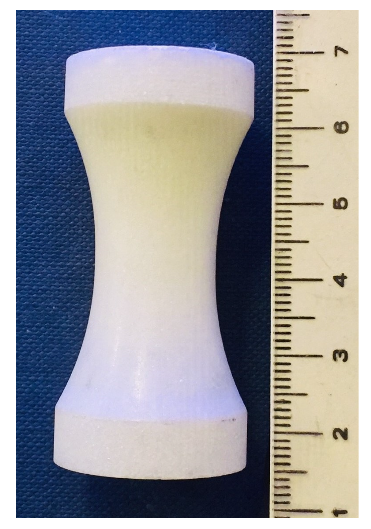
2.1. Rock Sample Used and Its Petrographic Characterization

The rock sample was cored to 25.1 mm diameter and 52.5 mm long from a large block of ‘Lorano Bianco’ statuary quality white Carrara marble in the direction designated a. The Carrara marble was measured by X-ray diffraction and found to be >99 wt% calcite. The porosity was measured by gravimetry to be less than 1%. The sample was ground into a ‘dog-bone’ shape (Figure 1) using a grinding wheel of 42 mm radius, so that the central diameter was 16.0 mm. The reduced section extends over a distance of 37.8 mm of the central part of the sample. This means that at the end of the deformation the differential stress was at a maximum in the centre of the specimen and decreased towards each end.
One of the outputs of post-deformation EBSD in the petrofabric analysis described below is the surface area of each of the 320 grains measured in a contiguous planar swath along the centre line of the specimen. Grain shapes were close to equant but with angular boundary shapes characteristic of grain growth under hydrostatic load. The areas were converted into Feret diameters [15]. These are the diameters of circles of the same area as each grain, and are widely used to represent planar grain size. Figure 2a shows the planar grain size distribution. The arithmetic mean grain size is 99 µm but the distribution is skewed to the coarser grain sizes. The range of grain sizes is 5 µm to 370 µm, with rather few grains represented above 250 µm. Planar distributions of grain sizes produced by normal grain growth tend to be close to Gaussian when plotted as square root grain diameter on the abscissa [16,17,18], and that is true of this case (Figure 2a). Mean square root grain size is 9.30 µm0.5 and standard deviation is 3.51 µm0.5. All of the grain size information reported here is the planar grain size; no stereological corrections for the effect of the two dimensional cut have been applied e.g., [8].
For this type of study it is important there be no significant crystallographic preferred orientation within the sample. The EBSD measurements made after deformation allowed the total crystallographic preferred orientation (CPO) of each grain within the external reference frame to be determined. There is one unique reference direction in the external frame, this is the orientation of the specimen axis that becomes the direction of the maximum compressive stress. Figure 2b shows the orientation of the specimen axis within the crystallographic reference frame of calcite (Inverse Pole Figure, IPF). Despite these measurements having been made after the specimen had been shortened by amounts varying up to 4% (see below, Section 2.2), this is not sufficient strain to produce a significant CPO. Except for some apparent clearing of grains from around the periphery of the projection, the distribution of points appears typical of a random sample from a uniform distribution, hence the specimen is expected to be approximately mechanically isotropic at the onset of deformation.

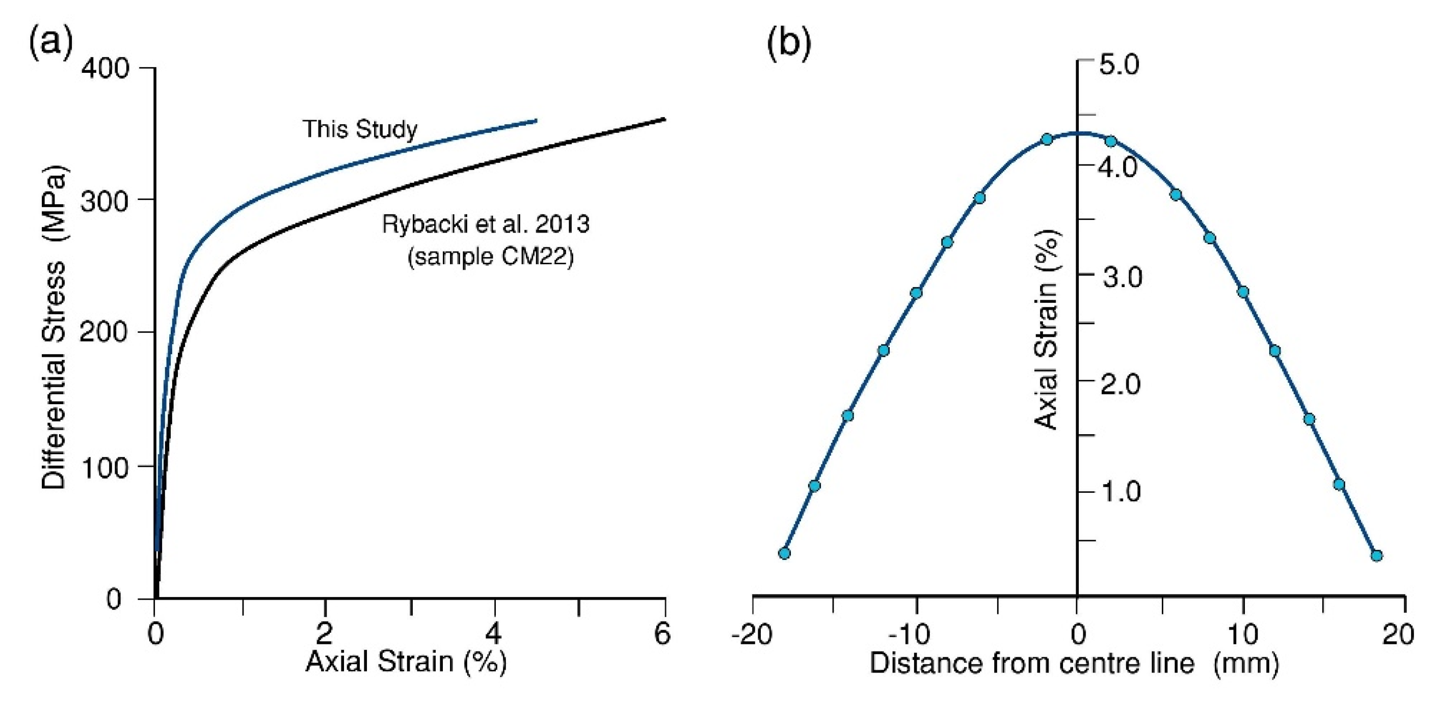
2.2. Sample Strength Characterization

The rock sample was deformed at 20 °C under axisymmetric compressive (irrotational strain) loading in a standard ‘triaxial’ rock deformation apparatus at a constant confining pressure of 225 MPa, applied by hydraulic oil. A heat-shrink rubber jacket was used to exclude oil from the pores of the rock. The nominal axial strain rate relative to the overall length of the specimen was 4.0 × 10⁻⁵ s−1.
The total nominal axial strain was 0.9%, but owing to the variable diameter of the rock cylinder, this is not uniformly distributed along the specimen length, but will be higher in the central portion, and lower towards the ends. The local axial strain is equal to the area strain, assuming homogeneous deformation at constant volume. This distribution of strain was calculated from measurements of the local cross-sectional diameter, and these were used to calculate the distribution of strain at the end of the test. The apparent axial stress/strain curve is shown in Figure 3a, with the differential stress calculated as for the final central diameter of 16.37 mm (local strain = 4.35%). Rybacki et al. [8] reported deformation experiments on Carrara marble from the same source. Their sample CM22 was deformed under the same conditions as this one, except that the confining pressure was higher, at 300 MPa. Their stress/strain curve is also shown on Figure 3a for comparison.
The principal stresses along the axis of the specimen are expected to be parallel and perpendicular to the specimen axis, whereas at the periphery of the sample, where the confining pressure acts normal to the free surface, they are expected to be parallel and perpendicular to that surface. Thus the stress trajectory pattern will be curved, as illustrated in Figure 4a, and the ( σ 2 = σ 3 ) surfaces will form a series of spherical caps. At all cross-sections through the specimen the axial force will be the same, thus the stress across all such spheroidal segments will be the force/cap area. The force in the middle of the specimen is the final stress (372 MPa) × the local area (210.3 mm2) = 78.2 kN. Differential stresses reported are estimated to be accurate to ± 1.5 MPa.
The area A of each spherical cap is given by A = 2 π R 2 ( 1 cos θ ) ,   where   R   and   θ are as defined in Figure 4a, and from which the distribution of axial stress along the centre line of the specimen at the end of the experiment can be calculated (Figure 4b).

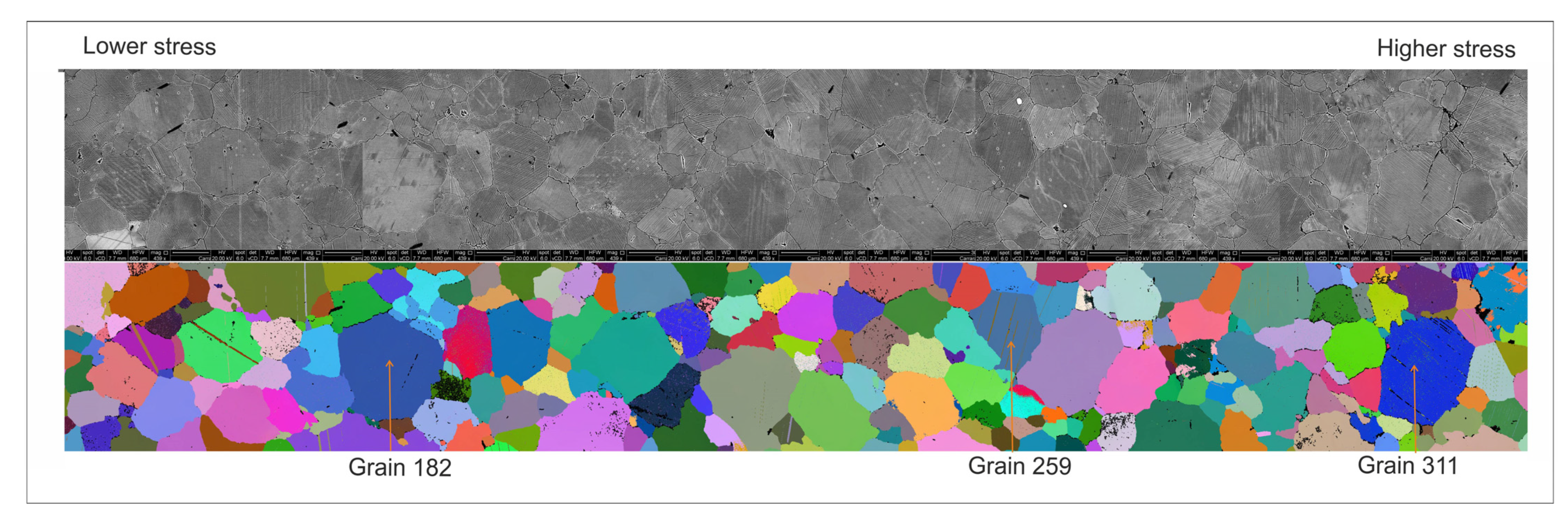
2.3. Electron Backscatter Diffraction (EBSD) Analysis

The deformed specimen was cut in half longitudinally and one half was polished with progressively finer diamond grits and finished with colloidal silica. This final polish removes near-surface defects from the sample material. EBSD data were collected on an FEI Quanta 650 field-emission gun scanning electron microscope equipped with Oxford Instrument’s HKL Channel 5 EBSD acquisition software and Nordlys Nano detector. An EBSD map was collected in a swath along the centre line of the specimen and consists of 10,514 × 600 measurements at a step size of 1 µm. Data were postprocessed by removing misindexed pixels that differ in orientation by >10° from all of their neighbours and then iteratively filling nonindexed pixels with >6 neighbours within the same grain. The resulting dataset has 99.12% of the points indexed as calcite, constituting over 6.2 million measurements. The width of the map is sufficient to encompass 2 or 3 of the larger diameter grains (Figure 5). Grains were numbered for identification, and a total of 320 grains were sampled without truncation.
Several different unit cell definitions can be used for calcite and these give rise to different crystallographic indices for a given crystallographic form. To avoid confusion it has become common to refer to crystallographic forms and axes using lower case letters. Some of these are shown (as crystallographic axes or poles to planes) on the pole figure in Figure 2b and Figure 6. c represents the unique crystal axis of trigonal symmetry, ±a1, a2, and a3 are the three crystallographic axes normal to c, ± m1, m2 and m3 are the planes of the trigonal prism, r1, r2 and r3 are the three cleavage rhombs, and f1, f2 and f3 are the three planes of the steep (dogtooth spar) form. The e form defines the poles to the three common twin planes in calcite, and is cozonal with two of the cleavage rhomb planes. Important angles are c^e = 26.25°, c^r = 44.5°, c^f = 63° [2]. Calcite belongs to the holosymmetric trigonal class, but the directions of the mutually orthogonal a2 and c crystallographic axes and the pole to the trigonal prism are convenient reference axis choices.
Crystallographic orientations of individual grains were recorded as three Euler angles E1, E2 and E3, using the Bunge convention [19,20]. These angles relate the crystallite orientation to the external reference frame. The external reference frame is defined by the specimen axis X, which is the direction of maximum applied stress, the Y axis which is normal to X and lies in the plane of the polished sample, and the Z axis which is normal to the polished sample surface. To define the rotations, initially the crystallographic m pole is set parallel to X, the crystallographic + a2 axis is set parallel to Y and crystallographic c axis is set parallel to Z (Figure 6b). In this position all Euler angles are initially zero. The labels X, Y and Z of the external reference frame also correspond to 1, 2 and 3 respectively commonly used in the subscript notation (unprimed axes), and in this case the mutually orthogonal m, a2 and c directions of the calcite crystal would be labelled 1′, 2′ and 3′ (primed axes) in the subscript notation. The use of only three Euler angles to represent crystallite orientation requires the order of the successive angular rotations to link the crystallographic and external reference frames to be specified [20]. The operation of the sequence of rotations yields the angular relationship as Euler angles linking the reference frame (unprimed axes) to the crystallographic orientation (primed axes) of each grain. Starting with the unprimed and primed axes in coincidence, the Euler angles specify the successive rotations by angles E1, E2 and E3 about the primed axes 3′–1′– 3′ successively, that are necessary to bring the grain into its observed orientation with respect the external reference frame.
Whilst graphical plotting and other mathematical operations can be carried out directly from Euler angles, it can be easier to work with direction cosine arrays (aij, where i, j = 1, 2, 3). Each of the direction angles (cos−1 aij) links a pair of unprimed and primed axes. The first subscript refers to one of the unprimed axes, and the second to one of the primed axes, thus there are nine direction cosines in total. The elements of the direction cosine array are related to the Euler angles by the expressions [19]
[ a 11 a 12 a 13 ] = [ cos ( E 3 ) cos ( E 1 ) cos ( E 2 ) sin ( E 1 ) sin ( E 3 ) cos ( E 3 ) sin ( E 1 ) + cos ( E 2 ) cos ( E 1 ) sin ( E 3 ) sin ( E 3 ) sin ( E 2 ) ] [ a 21 a 22 a 23 ] = [ sin ( E 3 ) cos ( E 1 ) cos ( E 2 ) sin ( E 1 ) cos ( E 3 ) sin ( E 3 ) sin ( E 1 ) + cos ( E 2 ) cos ( E 1 ) cos ( E 3 ) cos ( E 3 ) sin ( E 2 ) ]   and [ a 31 a 32 a 33 ] = [ sin ( E 2 ) sin ( E 1 ) sin ( E 2 ) cos ( E 1 ) cos ( E 2 ) ]
From the direction cosine array for each grain the orientation of the three potential twin planes in that grain can be calculated, together with the resolved shear stress factors and slip sense on each twin system, and the orientation of the trace of twin and other planes on the polished surface and its inclination with respect to that surface.
Whilst the EBSD data clearly allow the identification of the size, shape and orientation of the host grains, they also show twin lamellae when they are wide enough to be picked up by the 1 μm grid sample spacing (e.g., Figure 5). However, only 19 grains possessed twins wide enough to be detected in this way. The majority of twins induced in the deformation experiment were not detected by EBSD because they were generally thinner than the sampling step distance and/or thinner than the interaction volume of the electron beam. In contrast, the traces of twins were clearly visible in the electron-channelling orientation contrast images. These images, with examples presented in Figure 5 and Figure 7, were collected using a standard backscattered-electron detector at a short working distance of 7.7 mm to enhance orientation contrast through the electron-channeling effect. Twins appear as stripes that are either brighter or darker than the host grain due to differences in crystallographic orientation.
Having related the orientation of each host crystal to the three possible twin plane orientations, the expected orientations of the twin traces on the polished surfaces of the grains can be calculated, and used to test the observed linear traces. This procedure was performed for all host grains. The correspondence between observed and calculated twin traces would usually be within ±2°. In this way it was possible to determine twin plane orientations without requiring a direct EBSD measurement of the twinned crystal within the twin lamella. Figure 7 shows this analysis using the example of grain #259. In this case, calculated twin plane trace e3 corresponds with a single well-developed twin set.
The inclination of each of the possible twin plane(s) to the specimen surface was also calculated. The total number of observed twin traces across the width of each grain was counted manually, and the true spacing between the twins was calculated from the twin plane inclination and the apparent spacing between the twins on the specimen surface. In this way it was possible to determine the twinning activity in each grain, i.e., how many twin sets are present, the number of twins and their true spacing. To our knowledge this approach has not previously been employed in the analysis of twinning activity and twin orientations. It allows, for example, the calculation of the resolved shear stress and shear sense on all twin planes and allows discrimination between twins and traces of other planar features that might be seen, such as cleavage or slip surface traces.
The supplementary data file DFT.csv provides, for all of the measured grains, the identifying grain number, the EBSD-measured orientation data as Euler angles for host grain orientation and twin lamellae measured by EBSD, the X and Y coordinates of the position of each grain centroid, the X distance along the specimen axis to each grain centroid, the grain area, the Feret diameter and the differential stress on each grain. Additionally are tabulated; the crystallographic orientation as Euler angles of each twin lamella calculated from trace analysis, the inclination of each twin pole to the specimen surface, the apparent twin density (number of twins per mm) and the true twin density after correction for the twin plane orientation, Schmid factor information (with sign) for each twin, resolved shear stress on each twin, and the twin density data from Rowe and Rutter [6].

3. Analysis of Experimental Results

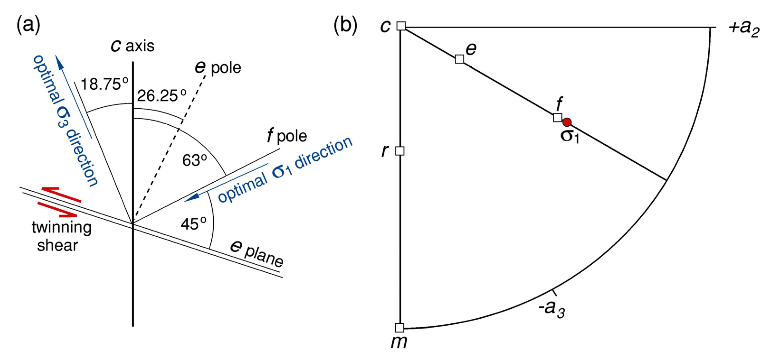
3.1. Turner/Weiss Analysis for Principal Stress Orientations

Turner [1] and Turner and Weiss [21] showed that the orientations of principal stresses could be determined from the relative orientations of twin lamellae and the c crystallographic axes of the host grains. This is a technique that has been widely and successfully applied e.g., [6,22,23,24,25,26,27]. The orientation of the displacement vector from deformation twinning is parallel to the zone axis containing an r plane and the e plane (Figure 6a), with the shear sense such as to displace the upper layers of the crystal towards the c-axis (defined as the positive sense of shear). The resolved shear stress τ acting along the twinning vector and in the twin plane is determined by the magnitude of the maximum differential stress ( σ 1 σ 3 ) , the angle λ between the maximum stress and the pole to e, and angle between the maximum stress direction and the slip vector, and is given by
τ = ( σ 1 σ 3 )   cos   λ   cos  
The product m = cos   λ   cos is called the Schmid factor and ranges between 0.0 and 0.5 [10]. The twinning transformation can only be produced with a positive sense of shear (Figure 6a). For each twinned grain the orientation of σ 1   and σ 3   can be estimated assuming the Schmid factor on that twin system is 0.5, in which case σ 3   lies 19° beyond c along the great circle ec, and σ 1   lies 45° beyond e along the great circle ce. When there are two, or even three, sets of twin lamellae, two or three predictions can be made for that grain.
The most accurate predictor of the principal stress orientations should be those grains for which the true Schmid factor is close to 0.5. Of the present sample of 320 grains in Carrara marble, 183 contained twin lamellae containing one or more twin sets with a positive sense of resolved shear stress, on the assumption that the principal stress orientations are the same in every grain. This includes the 19 grains bearing twin lamellae wide enough to be measured by EBSD, leaving 164 grains with thin twins, the orientations of which were obtained by the trace analysis method outlined above. These two groups of twins were analyzed separately (Figure 8), given that it was possible that the wider twins may have been produced by an earlier, natural loading event. The analysis of the 19 wide twin lamellae is shown in Figure 8a. Bearing in mind the small number of data available for the wide twins, the observed deviation of the best estimate of σ 1   orientation from the specimen axis is probably not sufficient evidence alone to conclude reliably that these twins probably formed from a previous deformation event.
The analysis of the narrow twin lamellae is shown in Figure 8b as the calculated optimal orientations of σ 1 required to produce the observed twins, assuming homogeneous stress from grain to grain. Data are contoured for the value of the Schmid factor for each twin plane. The best-fit calculated orientation of σ 1 is shown. In the plane orthogonal to σ 1   ,   σ 2   = σ 3   . The calculated orientation of σ 1 corresponds well with the long axis of the sample and also corresponds to the cluster of the highest values of Schmid factor. This correspondence also supports the presumption made for the Turner and Weiss [21] analysis that stress refraction from grain to grain is minor, as also demonstrated by [4]. Spiers [4] also showed that grains with a high Schmid factor on a twin system were preferentially more strained than grains with a small Schmid factor, with the former therefore taking up a larger fraction of the strain applied to the specimen as a whole. Therefore when twinning is active, stress is relatively homogeneous from grain to grain, but strains are markedly heterogeneous. In contrast at high temperatures, when mechanical weakness results in stresses too low to activate twinning [4,18], strains are homogeneous from grain to grain whilst stress orientations are markedly heterogenous. This leads to a transition in deformation-induced crystallographic preferred orientation (CPO) type when calcite rocks are deformed at temperatures too high to generate sufficient differential stress to activate twinning [4,18,28].
A further indication that grain-to-grain stresses are near-homogeneous is indicated by Figure 9. This is an inverse pole figure (equal angle upper hemisphere projection) showing the orientation of the axis of the test piece (the applied σ 1 direction) with respect to crystallographic directions of each grain in the specimen. Predicted combinations of positive sense Schmid factor on zero, one, two or three planes occupy areas on the projection separated by segments of great circles. Symbols representing grains are indicated according to the number of twin sets displayed. The distribution of these grains accords moderately well with the positions of boundaries calculated on the assumption of homogeneous stress.

3.2. Relations among Twinning Activity, Strain and Differential Stress Magnitude

3.2.1. Strain from Twinning and Use of Twin Volume Fraction to Infer Stress

Various microstructural characteristics of deformation twinning in calcite rocks have been used to make inferences about magnitude of plastic strain and differential stress. Groshong [3,9] devised a technique for estimating strains due to twinning in calcite aggregates by measuring the shear strain in individual, differently oriented grains from the aggregate total of twin widths and the characteristic angular shear associated with twinning. From those measurements the average strain attributable to twinning over the whole rock was calculated. The technique relies on being able to measure the widths of individual twins, and could not be applied to our sample experimentally deformed at 20 °C because virtually all of the twins were too thin to measure. Whilst even at low temperatures calcite twins tend to widen with strain [29], widening is inhibited when twins must emerge onto grain boundaries because they must generate dilatation in the grain boundaries, and this is resisted by elevated confining pressure. This effect leads to twin lamellae increasing in number to accommodate more strain.
It is well known that with increasing temperature calcite twins tend to become thicker within the grains [22]. To illustrate this effect, from a separate study Figure 10a shows such thick twins, widened after annealing at 600 °C, 200 MPa confining pressure, and pinched at the grain boundaries, thus avoiding steps appearing at the grain boundaries. Twin boundaries therefore become curved and irrational. Figure 10b shows the initially polished surface of a calcite grain in Carrara marble deformed at 700 °C, 200 MPa confining pressure [30], with a 10 µm grid impressed on the surface to reveal strain heterogeneities. Two twin lamellae show shear of the grid in the centre of the twin, but also strain-free twin-boundary migration away from the sheared lamellae, inferred to be driven by dislocation density developed in the host crystal volume [8]. To use the twin width to estimate shear strain in this case would lead to erroneous results.
As one of three techniques to use microstructural measurements of twins to infer differential stress, Rowe and Rutter [6] proposed a method based on the measurement of volume-percent of twins in experiments at elevated temperatures. The later observations of twin boundary migration without strain reported by Rutter [30] effectively negate that approach. Further, given the difficulty of measuring volume fraction of twins from thin twins produced in low bulk-strain experiments at low temperature, we conclude that paleostress measurement based on such measurements are probably impractical.

3.2.2. Twinning Incidence
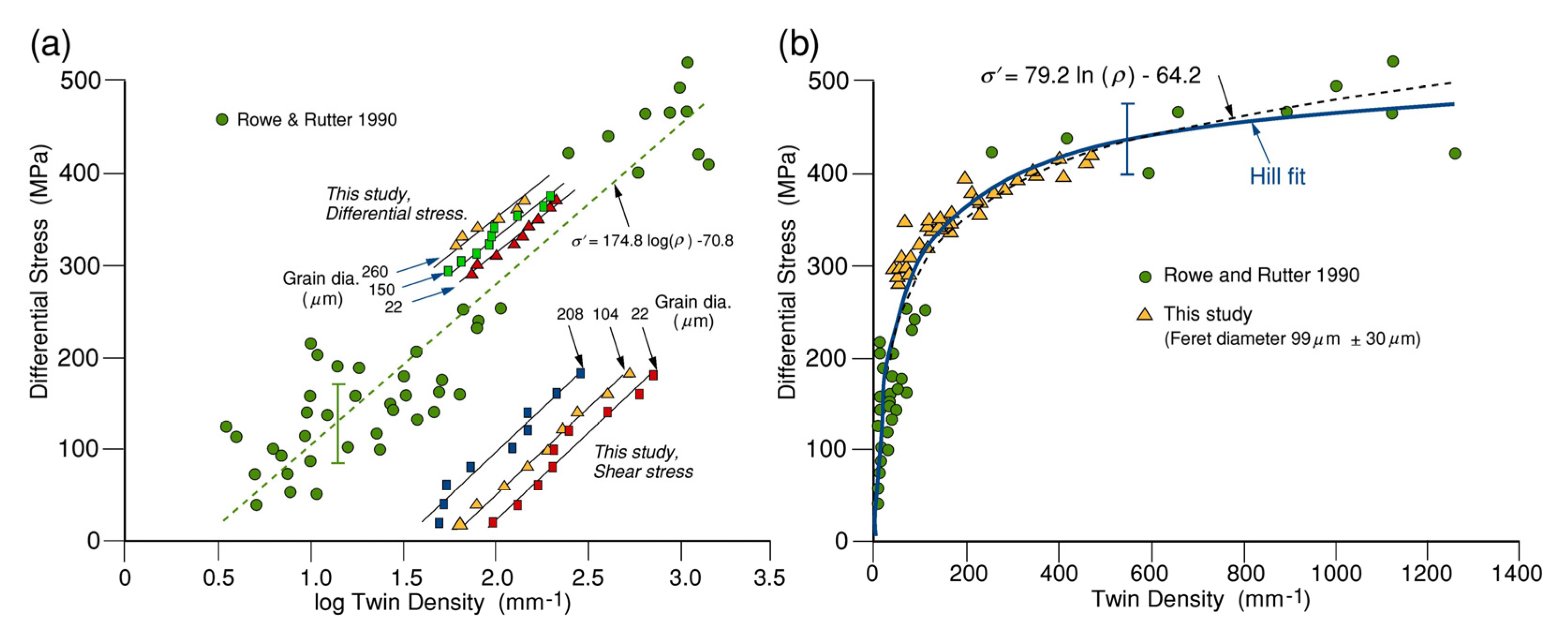
Rowe and Rutter [6] proposed two further approaches to twin paleopiezometry. One was based on the observation of twin incidence, that is the count of the fraction of grains that display twins within a particular grain size interval. From experiments carried out on three low porosity calcite rocks (Solnhofen limestone, Carrara marble and Taiwan marble), each with greatly different mean grain sizes, and covering a wide range of temperature and strain rate, it was clear that the threshold differential stress for the formation of twins observable in thin section was greater for finer-grained rocks and was almost independent of temperature and strain rate.
Similar observations have been made for twin incidence in austenitic steels (grain size dependence: [31,32]) and in iron, copper, zirconium and silver (temperature and rate insensitivity: review by Meyers et al. [33]).
The data acquired in the present study do not allow further evaluation of this approach for low temperatures and low strains, but from our dataset it is possible to observe the differential stress and the resolved shear stress necessary to produce the fraction of twinned grains developed in a particular grain size interval. A major deficiency of the measurements of Rowe and Rutter [6] was that the crystallographic orientation of each grain was not taken into account, but the twin incidence variation with differential stress and grain size for the whole population of grains could still be seen. In the present study, a substantial number of grains could be sampled only at and around the mean grain size of the population, and only for a low twin incidence. Figure 11 shows the differential stress and grain size ranges corresponding to a twin incidence of 20%, and these data are compared with those of Rowe and Rutter [6]. The uncertainties in these two datasets overlap and it can be seen that for grain sizes in the range 75–130 µm (mean grain size ±30 μm) the differential stress to produce twins in 20% of the grains is approximately 300 MPa.
The approaches to paleopiezometry tested by Rowe and Rutter [6] did not make any presumptions about a critical resolved shear stress for twinning, because it was clear that the differential stress necessary to produce twinning was dependent upon grain size. However, other approaches have been built around the concept of a critical resolved shear stress for twinning on the order of 10 MPa, usually based upon measurements of twinning initiation in large single crystals of calcite [2,7,34,35,36]. Inevitably these measurements led to the inference of low differential stress levels for twinning. De Bresser and Spiers [34] have criticised the adoption of a single CRSS value for twinning as a basis of paleopiezometry. In progressively finer-grained rocks of low porosity it is clear that twins do not form until high differential stresses have been applied; on the order of hundreds of megapascals for grain sizes smaller than 100 µm [6,8,10,37]. Propagating twin lamellae are geometrically like cracks, and will therefore be expected to produce long-range self-stress fields around their tips, and hence may be expected to be repelled by the proximity of grain boundaries in fine-grained polycrystals. Thus a consideration of effects of grain size must be implicit in any reliable paleopiezometry scheme.
It is also to be expected that ease of twinning will be affected by porosity, for twins can be nucleated at the stress concentrations that exist around pores. Experimental data on coarse-grained and porous rocks are therefore expected to result in high incidences of twins [7]. Confining pressure is also to be expected to affect behaviour. If dilatation of grain boundaries is facilitated by low effective pressures it will be easier for twin lamellae to penetrate such boundaries. Conversely, high effective hydrostatic pressures applied to porous rocks are likely to initiate twinning from the pores. For these reasons in the present study and others [8,38] a fairly high confining pressure in a low porosity rock was used to minimise complications from opening of grain boundaries.

3.2.3. Twin Density

The experimental data acquired in this study allow the relationships between twin density in each grain (number of twins per millimetre in each twin-bearing grain, measured normal to the twin plane) to be related to the resolved shear stress on each active twin system, total differential stress, and grain size. Almost half of the grains measured contain no twins at all. Figure 12a shows resolved shear stress, calculated from local differential stress multiplied by Schmid factor for each grain, for grains of Feret diameters lying in the range 73–150 µm, thus centred on the mean grain size. These are plotted against log twin density.
If we make the assumption that all of the thin twins observed have approximately the same thickness, the observed twin density in a grain is a measure of the shear strain in that grain. We might expect that for a limited range of grain sizes and applied stress, the shear strain would vary systematically with Schmid factor m. Figure 12b shows Schmid factor plotted against log twin density for two of the three possible twin sets at near constant stress and over a range of grain sizes ranging ±50 μm about the mean. There is a clear positive correlation, thus a higher Schmid factor and therefore a higher resolved shear stress along the twin displacement vector leads to higher intragranular strains due to twinning. Bear in mind that a logarithmic plot of twin density is used, and thus that the strains at high resolved shear stress are more than ten times greater than at low resolved shear stresses. Although the trend is approximately linear there is a wide scatter, as seen also in Figure 12a, and which is much greater than the estimated measurement accuracy of individual data points.
Inferred resolved shear stresses in this study cover a large range of magnitude, take into account the precise orientations of individual grains and involve data taken over only a small range of grain sizes. Therefore it was expected that this approach to twinning analysis would result in a strong correlation between twin density and stress with only small deviations with respect to a monotonic trend. Figure 12 shows that there is a linear trend but that it is accompanied by a large standard error in stress. This variability cannot be attributed to random errors of measurement. The mechanical data yield differential stresses measured to an estimated ±1.5 MPa, and the EBSD data yield orientations of twin planes and slip vector to within an estimated ±2°. The twin densities measured depend on counting all the twin lamellae intersecting the area within the observed grain diameter, then using the twin plane orientation to calculate the number of twins per millimetre counted normal to the that orientation. It is assumed that the twin density is uniform throughout the whole volume of a grain. Depending on grain size and orientation, for twin-bearing grains, counted numbers of twins typically lie in the range 1 to 40. Mis-counts of 2 or 3 might occur in heavily twinned grains, leading to an uncertainty of the order of perhaps 10%. Missing one twin amongst 5 would represent an error of 20% in less-twinned grains. Some twins did not completely traverse a grain, but were each counted as one twin. The global deviations about the best fit line are therefore far larger than the estimated uncertainty on individual data points (Figure 12), hence the scatter represents real departures from a unique relationship between twin density and shear stress. Note that as Schmid factors approach zero, resolved shear stresses must also approach zero, hence the reliability of shear stress measurement must decrease in such cases. This is particularly evident if the data are plotted on log/log axes.
Whilst there is a possible contribution from stress heterogeneity from grain to grain (already argued to be small), variabilities in twin densities might arise from random variations in the occurrence of nucleation points of twins on grain boundaries, and stress concentration effects arising from chance differences in orientation and hence relative hardness between adjacent grains. It is also possible that some twins that do not wholly traverse a grain might not intersect the surface of observation. Covey-Crump et al. [37] have pointed out that observed twins may nucleate over a range of magnitude of differential stress through progressive yield and the onset of strain hardening, thus there may be no unique relationship between twin occurrence and differential stress. The achievable accuracy of estimation of paleostresses based on twin density measurements may therefore be fundamentally limited by uncontrollable physical variables. Rybacki et al. [8] assembled a large amount of data on shear stress versus twin density from their own observations and from the literature that support the point made above.
To explore further the potential of using twin density as a basis for paleopiezometry, whilst accepting its evident limitations, graphical plots were prepared respectively showing
(a)
resolved shear stress versus Feret grain diameter, contoured for constant values of twin density, and of
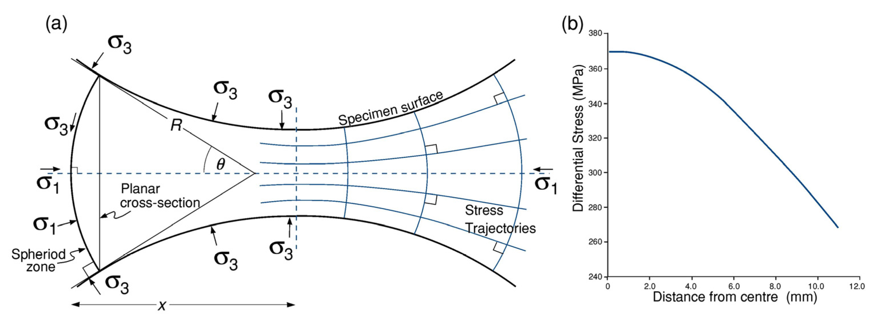
(b)
differential stress versus Feret grain diameter, again contoured for different constant values of twin density.
Figure 13 shows plots of (a) and (b) above. Locations of data points are indicated, and reflect the uneven distribution of sampled grain sizes. Relatively few large grains are present in the sample. The two plots in Figure 13 are similar in form, but whereas the plot of resolved shear stress extends over 0–180 MPa, the range of differential stress is 280–372 MPa. For the latter, in grains with more than one twin set it is the average twin lamellae count that is represented by the contouring.
In Figure 13a twin density increases with resolved shear stress but also, and somewhat surprisingly, decreases with grain size. The raw data plot shows the 164 twin sets with positive resolved shear stresses in individual grains. The remaining grains had no observable twin sets and a few had apparently negative shear sense twins, probably attributable to locally heterogeneous stresses. Departures from linearity on the plots of log twin density vs. resolved shear stress as shear stress approaches zero were apparent in the data for the coarser grain sizes, but surprisingly high twin densities are recorded in fine grains even at low resolved shear stresses. The same approach was adopted to analyze the twin density data but in terms of differential stress (Figure 13b).
In Figure 14a these two datasets are compared with the results presented by Rowe and Rutter [6]. After Gaussian smoothing to soften the short period fluctuations in twin density seen in Figure 13, followed by resampling, multiple linear regressions were carried out to fit resolved shear stress and differential stress data to Feret grain diameter and log twin density. The multiple linear regression fits are:
    τ = 375.8 + 190.2 log ρ + 0.412   d
  σ = 9.52 + 146.9 log ρ + 0.165   d    
where σ is differential stress (MPa), τ is shear stress (MPa), ρ is twin density (mm−1) and d is Feret grain diameter (mm). Standard errors in stress are respectively ±11.5 MPa and ±6.5 MPa, and depend on the degree of smoothing applied.
Equation (2) is plotted for three different grain sizes in Figure 14a. Separating grain sizes removes scatter that presumably arises in the Rowe and Rutter [6] dataset resulting from not differentiating between different grain size fractions. However, the locus and trend of the Rowe and Rutter [6] dataset, involving three different calcite rocks, is clearly comparable with the data of this study expressed in terms of differential stress.
In Figure 14 the data of [6] for twin densities are apparent twin densities counted on the cut surface of the rock section. There was no correction applied for the inclination of the twin planes to the section surface. However, the samples were all deformed to axial strains of 10% or more, which is sufficient to induce a degree of CPO. The rotations associated with CPO development would move e-poles towards parallelism with the sample surface (the e-maximum CPO type), which causes apparent twin density to converge towards the true twin density. Without this effect and when strains are small, and without calculating true inclinations of all twins, an approximation to the true twin density can be obtained by multiplying the apparent twin density by a factor √2.
Figure 14a also shows data relating resolved shear stress on the one or more twin sets in each twinned grain to the twin density. Each value of resolved shear stress can be multiplied by 2 to obtain the equivalent differential stress that would produce the same resolved shear stress on an ideally-oriented grain. The highest resolved shear stresses, where the Schmid factor is close to 0.5, correspond to the upper end of the twin density data expressed in terms of the differential stress, but lower resolved shear stresses are associated with higher twin densities than would be expected from the data in terms of differential stress. The plot of differential stress versus twin density derived from resolved shear stresses therefore underestimates twin density at progressively lower differential stress values, because no account is taken of the variable orientation of grains, but this does not significantly detract from the potential utility of the observed relationships as a paleopiezometer.
Figure 14b shows differential stress σ (= σ 1   σ 3   ) plotted against twin density, combining the data of this study with that of [6]. Their compatibility is self-evident. A good fit to the data is the exponential equation σ = 79.2 lnρ – 64.2, with a standard error in σ 1 of ±45 MPa, and valid down to a differential stress of about 30 MPa. This function has a finite intercept in ρ however, which is unrealistic. The three-parameter Hill function is particularly well suited to describing data with a strong localized curvature, and can be constrained to pass through (0, 0):
σ ( ρ ) = σ ( 0 ) + [ ( σ σ ( 0 ) ) ρ n ( k n + ρ n ) ]
where σ (= σ 1 σ 3 ) and stress σ is an upper limit to differential stress. k and n are adjustable parameters. Stress σ ( 0 ) is the value of differential stress (assumed to be zero) at zero twin density. The empirical Hill equation was devised to describe time-dependent uptake of drugs [39]. A non-linear least squares fit yielded the parameters σ = 545 MPa, k = 71.6 and n = 0.69, and the standard error in differential stress is ±41 MPa.

4. Discussion

4.1. Evaluation of the Turner (1953) Analysis for Principal Stress Orientations

The Turner [1] analysis for principal stress orientations has normally been applied by measuring optically the orientation of the host c axis and the e twin plane, and also noting the twin density. Although the Schmid factor is not usually determined, qualitatively higher twin densities are inferred to be associated with twin planes subjected to higher Schmid factors (Figure 12b). A good estimate of principal stress directions can usually be obtained by using only those grains with twin densities above an arbitrarily chosen number. However, in this study it has been possible to obtain Schmid factors for all twinned grains and it has been shown (Figure 8) that σ 1   directions estimated from twins with Schmid factors near to 0.5 very closely correspond to the known (applied) σ 1   direction.

4.2. Evaluation of Twinning Paleopiezometry Based on Twin Density

Having obtained linear relationships linking grain diameter and log twin density to respectively (a) resolved shear stress on the active twin systems and (b) applied differential stress, we can test the applicability of a paleopiezometer based on the measurement of twin density. Figure 15a,b show the variation of differential stress against distance along the specimen axis measured from the centre. Also shown are the respective distributions of differential stress obtained by back calculation from the raw twin density data for a restricted grain size range centred upon the mean. In (a) the resolved shear stress for an active twin system in each grain was calculated from Equation (1), then multiplied by the Schmid factor for that grain to obtain the differential stress. The division of the shear stress by the Schmid factor introduces a further source of uncertainty, especially when the Schmid factor is small. In (b) the differential stress was calculated by substituting the log twin density directly into Equation (2), and in this case no attention was given to the orientations of the grains from which the twin density measurements were taken. The Hill fit could alternatively be utilized to estimate the differential stress from the twin density measurements.
The estimated distribution of differential stress is clearly better for (b) (standard error in stress estimate for a linear fit = ±41 MPa) and the data are symmetrically distributed about the true line of differential stress variation along the specimen length. In (a) the standard error for a linear trend is ±95 MPa and the data points lie mostly beneath the known differential stress distribution. In both cases the scatter is an intrinsic property of the twin density measurements.
The procedure of back-calculating the differential stress from the original twin density data demonstrates the practicality of using twin density as a basis for a paleopiezometer. The procedure ‘re-introduces’ the intrinsic uncertainties in the relationship between stress and twin density so that its effect on the paleopiezometric tool can be seen. Clearly, the use of Equation (2) or the Hill equation (Equation (3)) will give the best estimate of the differential stress that acted upon the rock sample.

5. Conclusions

With the aim of investigating deformation twinning activity over a range of applied stresses, a dogbone-shaped specimen of Lorano Bianco Carrara marble was deformed in axisymmetric compression to a small strain (up to a maximum of 4%) at room temperature and at a confining pressure of 225 MPa. The sample was cut longitudinally to allow a tract containing 320 grain sections along the specimen axis to be analyzed using EBSD, with a step spacing of 1 µm. Crystallite orientations were determined using Oxford Instruments Channel5 software and crystallographic orientations were obtained as Euler angles. Twin orientations were determined by EBSD in the 19 grains that contained twin lamellae sufficiently wide to intercept and contain the incident electron beam, but in the majority of grains containing twin lamellae they were too narrow to be measured in this way. However, the orientations and number of twin lamellae in these grains could be determined by trace analysis. Thus from the host grain orientation and analysis of twin traces the Schmid factor and twin density for every set of twins encountered could be determined.
The applicability of the Turner [1] method for the determination of the orientation of principal stress axes was evaluated. The orientation of the principal stresses could be determined accurately particularly from those grains for which the Schmid factor approached 0.5.
The relationship between twin density (number of twin lamellae per millimetre) and (a) differential stress and (b) resolved shear stress on the twin planes was determined. Twin density increases with both (a) and (b), and smaller grain sizes record higher twin densities at a given stress level within the range of the dataset. Nevertheless, the overall incidence of twins is favoured by larger grain sizes. The onset of twinning requires the application of higher differential stresses in finer grained calcite rocks, but this does not reflect the ultimate density of twins in a given grain. Twinning only occurs when the sense of shear stress along the twin displacement vector is positive, and this was confirmed to be true such that the stress distribution amongst the grains is consistent with being near-homogenous.
The overall proportionalities observed between shear stress and twin density and between Schmid factor and twin density were subject to substantial non-systematic variability in measured twin densities. This scatter was inferred to be due to a small degree of stress refraction between grains coupled with more significant random differences from grain to grain according to the availability of twin nucleation points on grain boundaries. It is also not known at which points during progressive loading particular fractions of the twin assemblage formed. Nevertheless, after Gaussian smoothing of the data it was possible to obtain quantitative relations linking applied differential stress or resolved shear stress to twin density and grain size. The results were consistent with those reported by Rowe and Rutter [6], and the combined results of the two studies can be represented using the Hill equation. It became clear that too few grains, particularly at the larger sizes, were sampled for the purpose of this study, resulting in very uneven sampling by grain size. Future work using these methods should sample a much larger number of grains; at least 1000.
To evaluate possible use of the observed relationships as a practical twinning paleopiezometer and the likely uncertainties associated with it, the measured twin density and grain size measurements were applied to the above multiple regression fit to the data (Equations (1) and (2)), in order to evaluate how well analysis of twins would estimate differential stresses in the grains, had they not been known. The fit for the differential stress data gave a good representation of the initially applied differential stress and its variation along the length of the specimen (standard error on stress = ±41 MPa), but back-estimation of the applied stresses using the resolved shear stress data gave a much greater standard error of the estimate of differential stress (±95 MPa). The results of the present study, when combined with those of Rowe and Rutter [6], suggest that a practical paleopiezometer yielding differential stress based on twin density measurement would utilise the Hill equation (Equation (3)), or Equation (2).
This study has demonstrated the advantages of using EBSD and trace analysis to determine the orientation distribution of calcite host grains and twins they may contain. It has confirmed the utility of the Turner [1] analysis of twin/host relations for the estimation of the orientation of principal stresses, and also the applicability of twinning paleopiezometry based on twin density, whilst recognising that there are inherent limitations to the realizable accuracy of this approach.

Supplementary Materials

The following supporting information can be downloaded at: https://www.mdpi.com/article/10.3390/geosciences12060222/s1, Table S1: Data of all of the measured grains: Identifying grain number, the EBSD-measured orientation data as Euler angles for host grain orientation and twin lamellae measured by EBSD, the X and Y coordinates of the position of each grain centroid, the X distance along the specimen axis to each grain centroid, the grain area, the Feret diameter and the differential stress on each grain.

Author Contributions

E.R. conceived the study, carried out the rock mechanics experiment and drafting of the paper. E.R. and K.K. carried out the data processing and geometrical analysis. D.W. carried out the EBSD analysis. All authors have read and agreed to the published version of the manuscript.

Funding

This research received no external funding.

Data Availability Statement

All of the experimental data acquired in this research is freely accessible and collated in supporting datafile DFT.csv, which is downloadable from https://doi.org/10.5281/zenodo.5913355 (accessed on 15 May 2022).

Acknowledgments

Whilst this research was carried out, DW was in receipt of a NERC doctoral training grant NE/1528750/1 and KK a Manchester University student bursary. The EBSD measurements were made at the University of Leeds and the rock mechanics experimental work was carried out at the University of Manchester. Geoff Lloyd (Leeds), Julian Mecklenburgh and Stephen Covey-Crump (Manchester) provided helpful discussion and advice. The Carrara marble block used was provided by David Olgaard, then of ETH Zurich, who kindly distributed a number of blocks cut from a single large piece of ‘Lorano Bianco’ marble to laboratories around the world. We thank three anonymous reviewers reviewers and editor Olivier Lacombe for helpful and constructive comments on the paper.

Conflicts of Interest

The authors declare they have no conflict of interest.

References

  1. Turner, F. Nature and dynamic interpretation of deformation lamellae in calcite of three marbles. Am. J. Sci. 1953, 251, 276–298. [Google Scholar] [CrossRef]
  2. Turner, F.; Griggs, D.; Heard, H. Experimental deformation of calcite crystals. Bull. Geol. Soc. Am. 1954, 65, 883–934. [Google Scholar] [CrossRef]
  3. Groshong, R.H., Jr. Strain calculated from twinning in calcite. Geol. Soc. Am. Bull. 1972, 83, 2025–2038. [Google Scholar] [CrossRef]
  4. Spiers, C. Fabric development in calcite polycrystals deformed at 400 °C. Bull. Mineral. 1979, 102, 282–289. [Google Scholar] [CrossRef]
  5. Edmond, J.M.; Paterson, M.S. Volume changes during the deformation of rocks at high pressures. Int. J. Rock Mech. Min. Sci. 1972, 9, 161–182. [Google Scholar] [CrossRef]
  6. Rowe, K.; Rutter, E. Palaeostress estimation using calcite twinning: Experimental calibration and application to nature. J. Struct. Geol. 1990, 12, 1–17. [Google Scholar] [CrossRef]
  7. Ferrill, D.A. Critical re-evaluation of differential stress estimates from calcite twins in coarse-grained limestone. Tectonophysics 1998, 285, 77–86. [Google Scholar] [CrossRef]
  8. Rybacki, E.; Evans, B.; Janssen, C.; Wirth, R.; Dresen, G. Influence of stress, temperature, and strain on calcite twins constrained by deformation experiments. Tectonophysics 2013, 601, 20–36. [Google Scholar] [CrossRef]
  9. Groshong, R.H., Jr. Origin and Application of the Twinned Calcite Strain Gauge. Geosciences 2021, 11, 296. [Google Scholar] [CrossRef]
  10. Lacombe, O.; Parlangeau, C.; Beaudoin, N.E.; Amrouch, K. Calcite Twin Formation, Measurement and Use as Stress–Strain Indicators: A Review of Progress over the Last Decade. Geosciences 2021, 11, 445. [Google Scholar] [CrossRef]
  11. Rez, J.; Melichar, R.; Poelt, P.; Mitsche, S.; Kalvoda, J. Calcite twinning stress inversion using OIM (EBSD) data. Geolines 2005, 19, 100. [Google Scholar]
  12. Tielke, J.A. Development and Application of a Method for Determining Paleostress from Calcite Deformation Twins Using Electron Backscatter Diffraction. Master’s Thesis, South Dakota School of Mines, Rapid City, SD, USA, 2010; 124p. [Google Scholar]
  13. Evenson, A. Late Laramide Paleostress in Basement Rocks Determined from Calcite Twins using Electron Backscatter Diffraction, Lead-Deadwood Dome, South Dakota. Master’s Thesis, South Dakota School of Mines and Technology, Rapid City, SD, USA, 2011; 106p. [Google Scholar]
  14. Yan, S.; Zhang, B.; Zhang, J.; Wu, J.; Zhao, Z. Calcite Twins as a Tool for the Estimation of Paleostress Orientation on the Basis of Electron Backscatter Diffraction (EBSD) Technique. Bull. Geol. Sci. Technol. 2016, 35, 50–54. [Google Scholar]
  15. Walton, W. Feret‘s Statistical Diameter as a Measure of Particle Size. Nature 1948, 162, 329–330. [Google Scholar] [CrossRef]
  16. Andrade, E.N.; Aboav, D.A. Grain-growth of metals of close-packed hexagonal structure. Proc. R. Soc. Lond. 1966, A291, 18–40. [Google Scholar]
  17. Aboav, D.A.; Langdon, T.G. The planar distribution of grain-size in a polycrystalline ceramic. Metallography 1973, 6, 9–15. [Google Scholar] [CrossRef]
  18. Rutter, E.; Casey, M.; Burlini, L. Preferred crystallographic orientation development during the plastic and superplastic flow of calcite rocks. J. Struct. Geol. 1994, 16, 1431–1446. [Google Scholar] [CrossRef]
  19. Meyer, G.; Lee, H.Q.; Wehrend, W.R. A Method for Expanding a Direction Cosine Matrix into an Euler Sequence of Rotations; National Aeronautics and Space Administration Report NASA TM X-1384; NASA-Langley: Hampton, VA, USA, 1967; 14p. Available online: https://ntrs.nasa.gov/search.jsp?R=19670017935 2020-06-04T13:12:34+00:00Z (accessed on 6 May 2022).
  20. Bunge, H.-J. Texture Analysis in Materials Science, Mathematical Methods; Cuvillier Verlag: Göttingen, Germany, 1993; 595p. [Google Scholar]
  21. Turner, F.J.; Weiss, L.E. Structural Analysis of Metamorphic Tectonites; McGraw-Hill: New York, NY, USA, 1963; 545p. [Google Scholar]
  22. Burkhard, M. Calcite twins, their geometry, appearance and significance as stress-strain markers and indicators of tectonic regime: A review. J. Struct. Geol. 1993, 15, 351–368. [Google Scholar] [CrossRef] [Green Version]
  23. Tourneret, C.; Laurent, P. Paleostress orientations from calcite twins in the North Pyrenean foreland by the Etchecopar inverse method. Tectonophysics 1990, 180, 287–302. [Google Scholar] [CrossRef]
  24. Laurent, P.; Tourneret, C. Determining deviatoric stress tensors from calcite twins: Application to monophased synthetic and natural polycrystals. Tectonics 1990, 9, 379–389. [Google Scholar] [CrossRef]
  25. Nissen, H.U. Dynamic and kinematic of crinoids stems in a quartz graywacke. J. Geol. 1964, 72, 346–368. [Google Scholar] [CrossRef]
  26. Lacombe, O.; Laurent, P. Determination of deviatoric stress tensors based on inversion of calcite twin data from experimentally deformed monophase samples: Preliminary results. Tectonophysics 1996, 255, 189–202. [Google Scholar] [CrossRef]
  27. Laurent, P.; Kern, H.; Lacombe, O. Determination of deviatoric stress tensors based on inversion of calcite twin data from experimentally deformed monophase samples, Part II. Axial and triaxial stress experiments. Tectonophysics 2000, 327, 131–148. [Google Scholar] [CrossRef]
  28. Lister, G.S. Texture transitions in plastically deformed calcite rocks. In Proceedings of the 5th International Conference on Texture of Materials, Aachen, Germany, 28–31 March 1978; Gottstein, G., Lücke, K., Eds.; Springer: Berlin, Germany, 1978; Volume II, pp. 199–210. [Google Scholar]
  29. Parlangeau, C.; Dimanov, A.; Lacombe, O.; Hallais, S.; Daniel, J.M. Uniaxial compression of calcite single crystals at room temperature: Insights into twinning activation and development. Solid Earth 2019, 10, 307–316. [Google Scholar] [CrossRef] [Green Version]
  30. Rutter, E.H. Experimental study of the influence of stress, temperature, and strain on the dynamic recrystallization of Carrara marble. J. Geophys. Res. 1995, 100, 24651–24663. [Google Scholar] [CrossRef]
  31. Rahman, K.M.; Vorontsov, V.A.; Dye, D. The effect of grain size on the twin initiation stress in a TWIP steel. Acta Mater. 2015, 89, 247–257. [Google Scholar] [CrossRef] [Green Version]
  32. Chen, J.; Dong, F.-T.; Liu, Z.Y.; Wang, G.D. Grain size dependence of twinning behaviors and resultant cryogenic impact toughness in high manganese austenitic steel. J. Mater. Res. Technol. 2021, 10, 175–187. [Google Scholar] [CrossRef]
  33. Meyers, M.A.; Vöhringer, O.; Lubarda, V.A. The onset of twinning in metals: A constitutive description. Acta Mater. 2001, 49, 4025–4039. [Google Scholar] [CrossRef]
  34. de Bresser, J.; Spiers, C. Slip systems in calcite single crystals deformed at 300–800 °C. J. Geophys. Res. Solid Earth 1993, 98, 6397–6409. [Google Scholar] [CrossRef]
  35. Jamison, W.R.; Spang, J. Use of calcite twin lamellae to infer differential stresses. Geol. Soc. Am. Bull. 1976, 87, 868–887. [Google Scholar] [CrossRef]
  36. Laurent, P.; Bernard, P.; Vasseur, G.; Etchecopar, A. Stress tensor determination from the study of e-twins in calcite: A linear programming method. Tectonophysics 1981, 78, 651–660. [Google Scholar] [CrossRef]
  37. Covey-Crump, S.; Schofield, P.; Oliver, E. Using neutron diffraction to examine the onset of mechanical twinning in calcite rocks. J. Struct. Geol. 2017, 100, 77–97. [Google Scholar] [CrossRef] [Green Version]
  38. Schuster, R.; Habler, G.; Schafler, E.; Abart, R. Intragranular deformation mechanisms in calcite deformed by high-pressure torsion at room temperature. Mineral. Petrol. 2020, 114, 105–118. [Google Scholar] [CrossRef] [Green Version]
  39. Gadagkar, S.R.; Call, G.B. Computational tools for fitting the Hill equation to dose–response curves. J. Pharmacol. Toxicol. Methods 2015, 71, 68–76. [Google Scholar] [CrossRef] [PubMed] [Green Version]
Figure 1. Geometrical form of the sample of Carrara marble deformed in axial compression for this study (cm scale).
Geosciences 12 00222 g001
Figure 2. (a) Frequency distribution of the 320 Feret grain diameters in the sample of Carrara marble, with frequency plotted against grain diameter in blue, and against square root grain diameter in green. The green dashed line is a Gaussian curve for comparison, with the same mean and standard deviation as the square root grain size plot. The arithmetic mean grain diameter (99 μm) is indicated; (b) Inverse pole figure of calcite (upper hemisphere equal angle projection) showing the orientations of all 320 measured grains with respect to the specimen axis.
Geosciences 12 00222 g002
Figure 3. (a) Differential stress versus axial strain for the central 20 mm of the length of the specimen, where most of the ductile strain is accumulated. With respect to the overall specimen length the total strain at the end of the test is 0.9%. The stress/strain curve is compared with that of Carrara marble specimen CM22 of Rybacki et al. [8], which was deformed under similar conditions; (b) The distribution of permanent axial strain along the length of the specimen from post-test measurements of change in radial dimensions of the specimen, assuming deformation at constant volume.
Geosciences 12 00222 g003
Figure 4. (a) Schematic illustration of the form of the principal stress trajectories within the specimen. The axial force is distributed over the area of the ( σ 2 = σ 3 ) segments of spherical surfaces, the area of each of which is a function of x and must be calculated in order to determine the local σ 1   ( x ) ; (b) Calculated variation of axial stress σ 1 with distance from the centre of the specimen, where the axial stress is highest.
Geosciences 12 00222 g004
Figure 5. Example of grains sampled for EBSD analysis in the central region of the sample. The upper image shows electron channelling contrast. Traces of twin lamellae can be seen inside most grains and there is no evidence of significant microcracking nor grain boundary dilatation. The lower image is an Euler angle image, in which red-green-blue values are assigned based on the magnitude of each Euler angle. Three grains have been labelled by their number identifiers, by way of illustration. Most of the grains do not show twin lamellae visible in the Euler image, because most twins are too thin to be measured by the incident electron beam. The length of the portion of the section shown is 4.61 mm.
Geosciences 12 00222 g005
Figure 6. (a) The crystallographic zone containing poles to e and f, the calcite c-axis and the slip vector for twinning (which lies on the e-plane), to show angular relations. e-twinning can only occur with the shear sense shown, thus the optimal orientation of σ 1 for twinning lies on the zone plane at 45° to the e-pole, close to the f-pole; (b) Upper hemisphere equal-area projection of calcite showing the relations between c- and a-axes, and the poles to planes e, f and the trigonal prism m. The position of σ 1 in the optimal orientation for twinning is shown.
Geosciences 12 00222 g006
Figure 7. Orienting twin planes by trace analysis. Image of grain #259 (also shown in Figure 5) showing traces of one set of thin twin lamellae, together with the expected traces of the three possible twin planes (e1, e2, e3), the orientations of which were calculated from the host grain orientation. Trace e3 corresponds to the orientation of the observed twin plane traces.
Geosciences 12 00222 g007
Figure 8. (a) Upper hemisphere, equal angle projection of orientations of σ 1   ,   σ 2   and σ 3   directions from analysis of 19 grains containing wide twins that were measured during EBSD scans. The three orthogonal eigenvectors shown correspond to the orientations of the estimated principal stress directions; (b) Upper hemisphere, equal angle projection of orientations of σ 1 directions from analysis of the 164 grains containing new twin lamellae that could not be measured in the EBSD analysis because they were too thin to be detected. Instead, the twin plane orientations were established by analysis of the traces of the twin lamellae on the specimen surface together with the host grain orientations. The data are grouped according to the value of the Schmid factors resolved along the slip directions on the twin planes. The contours are not density contours but lines separating grains with progressively higher Schmid factors. The best estimate of σ 1 lies in the group of points for which the Schmid factor exceeds 0.4, and it fits well with the known orientation of σ 1 applied to the test piece. Eigenvectors for the clustered data define the orientations of the principal stresses. σ 2 is taken to be equal to σ 3 .
Geosciences 12 00222 g008
Figure 9. Inverse pole figure of σ 1 directions plotted in the crystallographic reference frame. The figure shows those areas for which a positive Schmid factor applies to 0, 1, 2 or 3 sets of potential twin lamellae, assuming homogeneous stress. σ 1 directions are coded according to the number of twin systems active in the grain.
Geosciences 12 00222 g009
Figure 10. (a) Optical micrograph of Carrara marble (crossed polars) experimentally shortened 27% at 420 °C then annealed under hydrostatic pressure at 600 °C, showing thickening of initially thin twins by twin boundary migration without strain. This leads to irrational twin boundaries especially near the host grain boundaries, where they pinch to avoid introducing steps to the host grain boundaries (image: Dr. S. J. Covey-Crump); (b) Surface of a calcite grain in Carrara marble, polished and impressed with a 10 µm grid before deformation at 700 °C to reveal strain heterogeneities. Two twin lamellae show shear of the grid where the twins nucleated, plus dynamic migration of the twin boundary without strain.
Geosciences 12 00222 g010
Figure 11. Relationship between differential stress and grain size for a twinning incidence of 20% (i.e., 20% of the grains in a particular grain size band contain twin lamellae). Thus at a given differential stress larger grains are more likely to contain twins, but there is no implication of the number of such twins. Shown are data of Rowe and Rutter [5] and the rather more restricted measurements that could be made on either side of the mean grain size in the present study.
Geosciences 12 00222 g011
Figure 12. (a) Relationship between log twin density (ρ) and resolved shear stress (τ) along the twinning vector direction (twin sets #1 and #2) in 32 grains centred on the mean grain size (99 μm).; (b) Schmid factor for twins in two twin sets (#1 and #3) plotted versus log twin density in 37 grains centred on the mean grain size, and for differential stresses in the range 360 to 372 MPa. Taking twin density as a proxy for shear strain if twin thicknesses are constant, shear strain increases with Schmid factor at constant stress and grain size.
Geosciences 12 00222 g012
Figure 13. (a) Resolved shear stress along the twinning vector plotted against grain size (Feret diameter) and contoured for twin density (mm−1). Individual grains are shown as black points. There are few large grains included in the traverse. There is a general trend of twin density increasing with shear stress and decreasing with grain size, plus short-period fluctuations in twin density, corresponding to the scatter shown in Figure 12; (b) Differential stress plotted against grain size (Feret diameter) and contoured for twin density (mm−1). General behavioural trends are the same as in (a).
Geosciences 12 00222 g013
Figure 14. (a) Data of Rowe and Rutter [6] relating differential stress to log twin density for three calcite rocks. These data are compared with those from this study, shown as Gaussian smoothed differential stress data for three different grain size bands fitted to log twin density by multiple linear regression. Also shown are fits to smoothed resolved shear stress data (using the same stress scale), again for three grain size bands; (b) Linear plot of differential stress against twin density for the data of Rowe and Rutter [6] plus the data of this study referred to the grain size band centred on the mean grain size. The data are fitted to the exponential function shown (dashed curve), but also fitted to the Hill equation (Equation (3)), constrained to pass through the origin (0, 0) (dark blue curve).
Geosciences 12 00222 g014
Figure 15. Back calculation of the variation in differential stress with distance along the sample axis using twin density data (twin set #1): (a) Using measured shear stress resolved along the twin displacement vector and shear stress calculated from Equation (1), Schmid factors calculated from measured angles λ and ; set of most frequent twins in 40 grains. Standard error in stress ±95 MPa; (b) All of the twin sets in all of the 181 twinned grains, Differential stresses calculated from Equation (2), Standard error in stress ±41 MPa.
Geosciences 12 00222 g015
Publisher’s Note: MDPI stays neutral with regard to jurisdictional claims in published maps and institutional affiliations.

