Article

Unsupervised Machine Learning, Multi-Attribute Analysis for Identifying Low Saturation Gas Reservoirs within the Deepwater Gulf of Mexico, and Offshore Australia

School of Geosciences, University of Oklahoma, 100 East Boyd Street, RM 710, Norman, OK 73019, USA
*
Author to whom correspondence should be addressed.
Geosciences 2022, 12(3), 132; https://doi.org/10.3390/geosciences12030132
Submission received: 10 January 2022 / Revised: 7 March 2022 / Accepted: 8 March 2022 / Published: 14 March 2022
(This article belongs to the Section Geophysics)

Abstract

:
An effective method of identifying and discriminating undersaturated gas accumulations remains unresolved, resulting in uncertainty in hydrocarbon exploration. To address this problem, an unsupervised machine learning multi-attribute analysis is performed on 3D post-stack seismic data over several blocks within the deepwater Gulf of Mexico and within the Carnarvon Basin, offshore Australia. Results reveal that low-saturation gas (LSG) reservoirs can be discriminated from high-saturation gas (HSG) reservoirs by using a combination of instantaneous attributes that are sensitive to small amplitude, frequency, and phase anomalies with self-organizing maps (SOMs). This methodology shows promise for de-risking prospects, even if it is not quantitative, particularly in frontier and exploration basins where wells may not exist or be very limited. However, this method only proved to be successful within the Gulf of Mexico and yielded limited results in the Carnarvon Basin. This difference is most likely due to the Carnarvon Basin having a different amplitude response resulting from a different burial history and fluid saturations when compared to the Gulf of Mexico. Therefore, this method is non-transferrable, and a different combination of attributes may be needed in other LSG-prone basins.

1. Introduction

The discrimination of low-saturation gas (LSG) reservoirs (less than 25%) from commercial quantities of gas remains one of the most challenging problems in petroleum exploration [1]. The ambiguity of LSG is primarily due to the elastic properties of gas, in particular the bulk modulus. The bulk modulus is a measure of the rock’s incompressibility when a force such as a seismic wave is applied. Due to the elastic properties of the gas’s bulk modulus on the bulk rock, a small, uneconomical, amount of hydrocarbon gas included in the pore space of the reservoir rock will reflect seismic energy back to the surface in a similar manner to a larger, and economical, accumulation of gas in the pore space (Figure 1). These rock physics relationships, with the inclusion of gas, will cause an LSG reservoir to have a similar seismic amplitude response to that of a commercial, high-saturation gas (HSG) reservoir [2,3]. The seismic reflection in both the LSG and HSG accumulations creates a bright amplitude anomaly within certain lithology and pressure regimes within the Gulf of Mexico and within the Scarborough gas field, offshore Australia [2,3,4]. These amplitude responses were analyzed within two producing fields in the Gulf of Mexico and the Scarborough gas field, offshore Australia (Figure 2A,B).
There have been several amplitude and rock physics analyses performed in the past to better characterize LSG in the subsurface with limited success under specific conditions that cannot be applied in a typical exploration scenario [3,5,6,7]. In recent years, machine learning techniques have gained a significant foothold within the geoscience community. Recent studies have shown promising applications of machine learning techniques to reflection seismic data to aid in the interpretation of geologic patterns [8,9,10,11]. Some of these applications are at the sub-seismic resolution scale since machine learning works on a sample interval basis, as opposed to being limited by the seismic wavelet [8,12].
This study aims to exploit the advances of machine learning and multi-attribute seismic analyses to test the limits and determine if small seismic waveform variations can be detected and properly attributed to the low- and partially-saturated gas reservoirs.

2. Geologic Settings

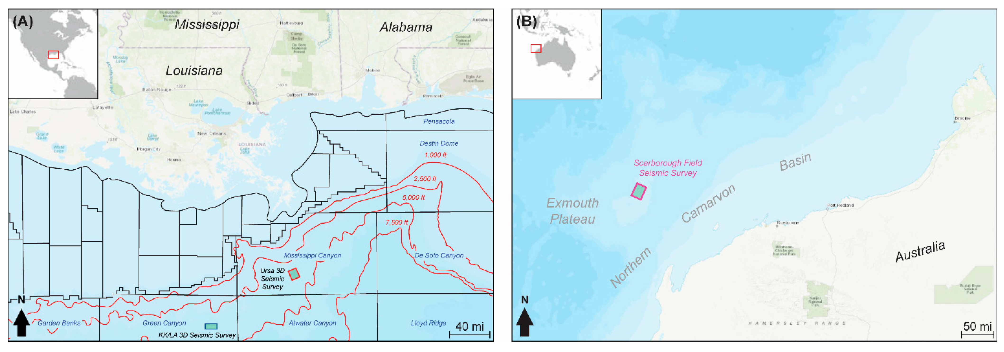
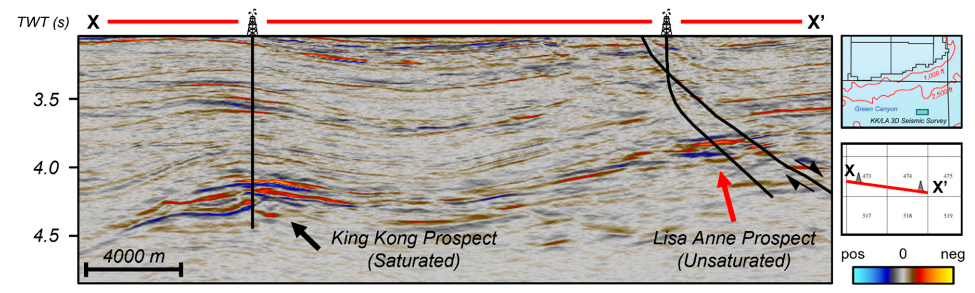
2.1. King Kong and Lisa Anne Prospects, Offshore Gulf of Mexico

The King Kong and Lisa Anne (KK/LA) prospects lie approximately 160 mi (257 km) south of New Orleans, within Green Canyon Blocks 473 and 474, offshore of the Gulf of Mexico (Figure 2A and Figure 3). These prospects occur in Plio-Pleistocene age sediments, share the same geologic model, and are mapped on the same reflector in seismic data. They are deepwater sand reservoirs that were deposited in a minibasin from a northerly source controlled by underlying salt bodies [3]. While the King Kong Prospect is a structural four-way closure, the Lisa Anne Prospect is positioned on the hanging wall of a large normal fault (Figure 3). Sand quality within both reservoirs is excellent, with porosities of roughly 30% [3]. Although both prospects appear to have similar seismic amplitude anomalies, the Lisa Anne proved to be an uncommercial prospect, having only about 5–25% gas saturation [3].

2.2. Ursa Gas Field, Offshore Gulf of Mexico

The Ursa field is a prolific producing deepwater field located approximately 130 mi (210 km) southeast of New Orleans within the Mississippi Canyon, offshore Gulf of Mexico (Figure 2A). The deepwater depositional environment of the Mars–Ursa intraslope basin is controlled by cycles of salt tectonics as well as turbidites. Amalgamated channelized sands and sheet sands act as reservoirs for the system and are overlain by condensed sections [13]. Within the Ursa Well #1, several hydrocarbons pay intervals, occurring at depths of 12,000 ft and from 17,000 to 20,000 ft within Pliocene to Miocene age sands. These are stacked pinch-out reservoirs against salt-bounded mini-basin flanks, similar to the play observed in the King Kong/Lisa Anne prospects. Sand quality is also excellent within the field, with an approximate porosity of 25% [13]. However, well log and AVO analysis revealed that one of the upper reservoir intervals was an LSG interval as the velocity was lower than the oil-saturated intervals (Figure 4) [2].

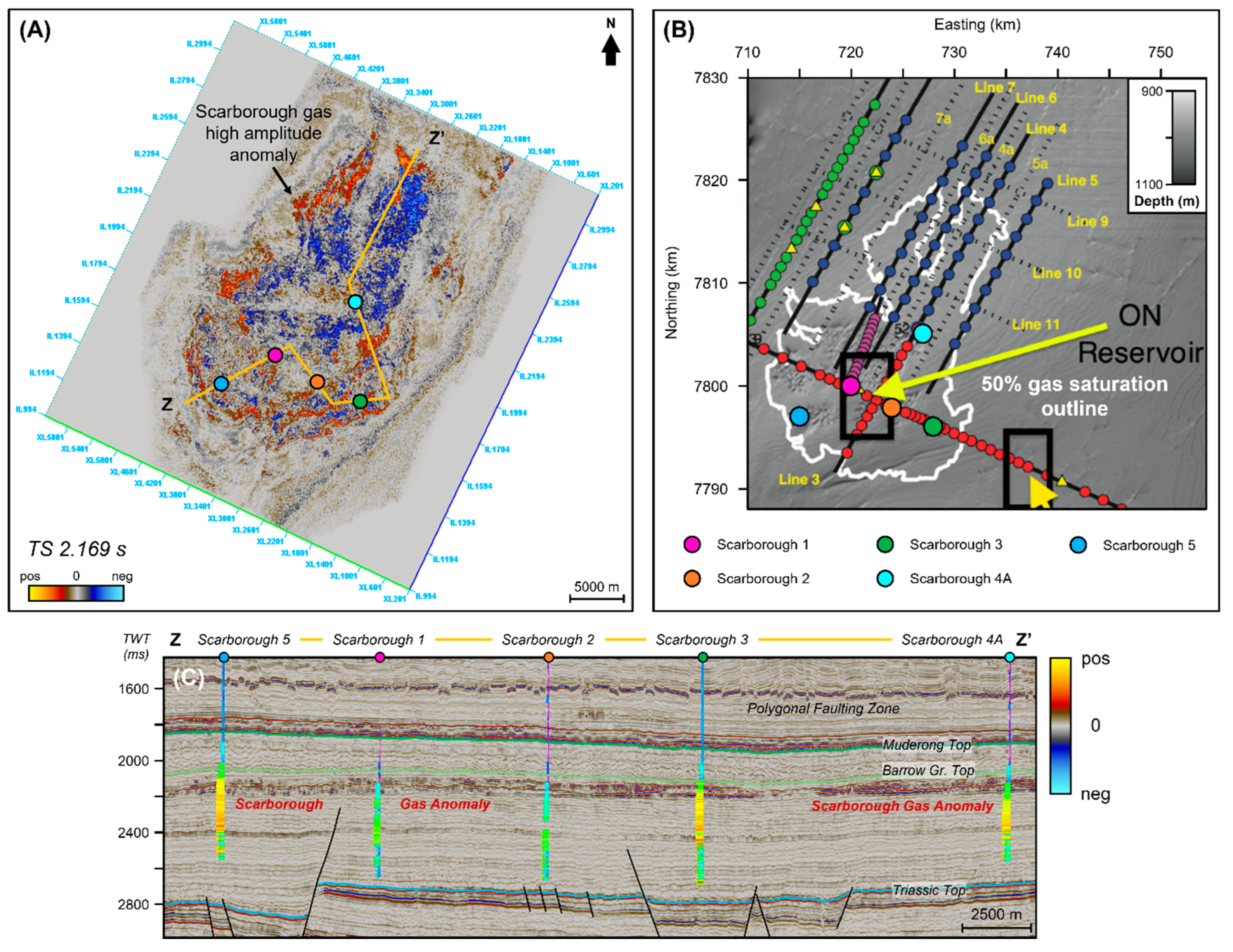
2.3. Scarborough Gas Field, Offshore Australia

The Scarborough gas field is situated on the Exmouth Plateau, in the Carnarvon Basin, offshore Australia (Figure 2B) [14]. The plateau is a passive margin between continental and oceanic crust that was formed as a result of the break-up of Australia and India. Sub-horizontal detachment faults dipping towards the Australian continent undercut the plateau at a depth of approximately 6.2 mi (10 km) where the continental crust transitions into oceanic crust [15]. The plateau, with dimensions of approximately 248 mi by 372 mi (400 km by 600 km), is bounded by transform faults toward the northeast and southwest [4]. A complex series of extension, fracture, uplift, truncation, and subsidence events have affected the plateau since the Mesozoic era [4].
The Scarborough reservoir is a three-tiered fan sequence that consists of Early Cretaceous deepwater turbidite sands deposited in a basin-floor fan setting [16]. With a water depth of about 1970 ft (900 m) and situated from 6240 to 6570 ft (1900 to 2000 m) below sea level, the reservoir is roughly 65 to 100 ft (20 to 30 m) thick [4,14,16]. These turbidite sands were sourced from the fluvio-deltaic Barrow Group, located approximately 31 mi (50 km) south of the field [14]. The Lower Fan unit contains the majority of the gas-in-place with porosities of 20–30% and is overlain by lower net-to-gross and lower quality Middle and Upper Fans [14,17]. The areal extent of the reservoir (a gas saturation higher than 50%) was defined using five exploration wells and available 3D seismic coverage (Figure 5A–C) [4].
The geologic backgrounds for the KK/LA and Ursa fields are fairly similar to one another, demonstrating comparable porosities, traps, and depths. However, the Scarborough field is significantly shallower with a different basin history and may illustrate a different amplitude response from the Gulf of Mexico fields.

3. Methodology

3.1. Available Data

Three, full-stack 3D datasets will be used for analyzing the varying amplitude responses of different gas saturations within the Gulf of Mexico, offshore United States and in the Carnarvon Basin, offshore Australia. While gathers and angle-stacks would be beneficial for our analysis, they were unavailable and were therefore not included in this study. Well logs for the King Kong and Lisa Anne as well as the Ursa Field were also unavailable as they are proprietary. However, a total of five wells were used in Scarborough gas field, offshore Australia.
Within the Gulf of Mexico, two surveys will be used. The G3D201407-02 3D, also known as the Green Canyon Phase II, post-stack seismic survey was collected in 1989 by Western Geophysical and covers approximately 580 mi2 (1500 km2) in the Gulf of Mexico (Figure 2A). This dataset covers the KK/LA prospects. The processing was also conducted by Western Geophysical and had a recording length of 9.5 s using a 4 ms sampling rate. The dataset is positive standard polarity. The second dataset, the G3D1304-002A through C survey, also known as the Shell Mississippi Canyon survey, was collected in 1988 by Shell and covers roughly 420 mi2 (1089 km2) in the Gulf of Mexico (Figure 2A). This dataset covers the Ursa gas field. The processing was conducted by Shell and had a recording length of 9.6 s using a 4 ms sampling rate. The dataset is positive standard polarity.
Within the Scarborough gas field, offshore Australia, the Scarborough 3D (HEX03A) seismic survey will be used to examine varying levels of gas saturation. The dataset was acquired and processed by WesternGeco Australia between March and July 2004. This survey covers approximately 351 mi2 (910 km2) and is located about 92 mi (240 km) north of Barrow Island (Figure 2B). Ten, 4000 m long streamers were used, at a separation of 75 m and a depth of 6.5 m. The acquisition energy source used a dual 3000 cubic inch Input-Output (IO) sleeve-air source, clustered arrays. The array centers were 50 m apart at a depth of 5 m. This energy source was fired every 18.75 meters along the pre-plotted survey line. The operating pressure of the towed source array was 2000 psi. The survey had a recording length of 6.1 s using a 3 ms sampling rate. The dataset has negative standard polarity. Five wells were used for this study, which all contained gamma rays, resistivity, density, and neutron porosity.

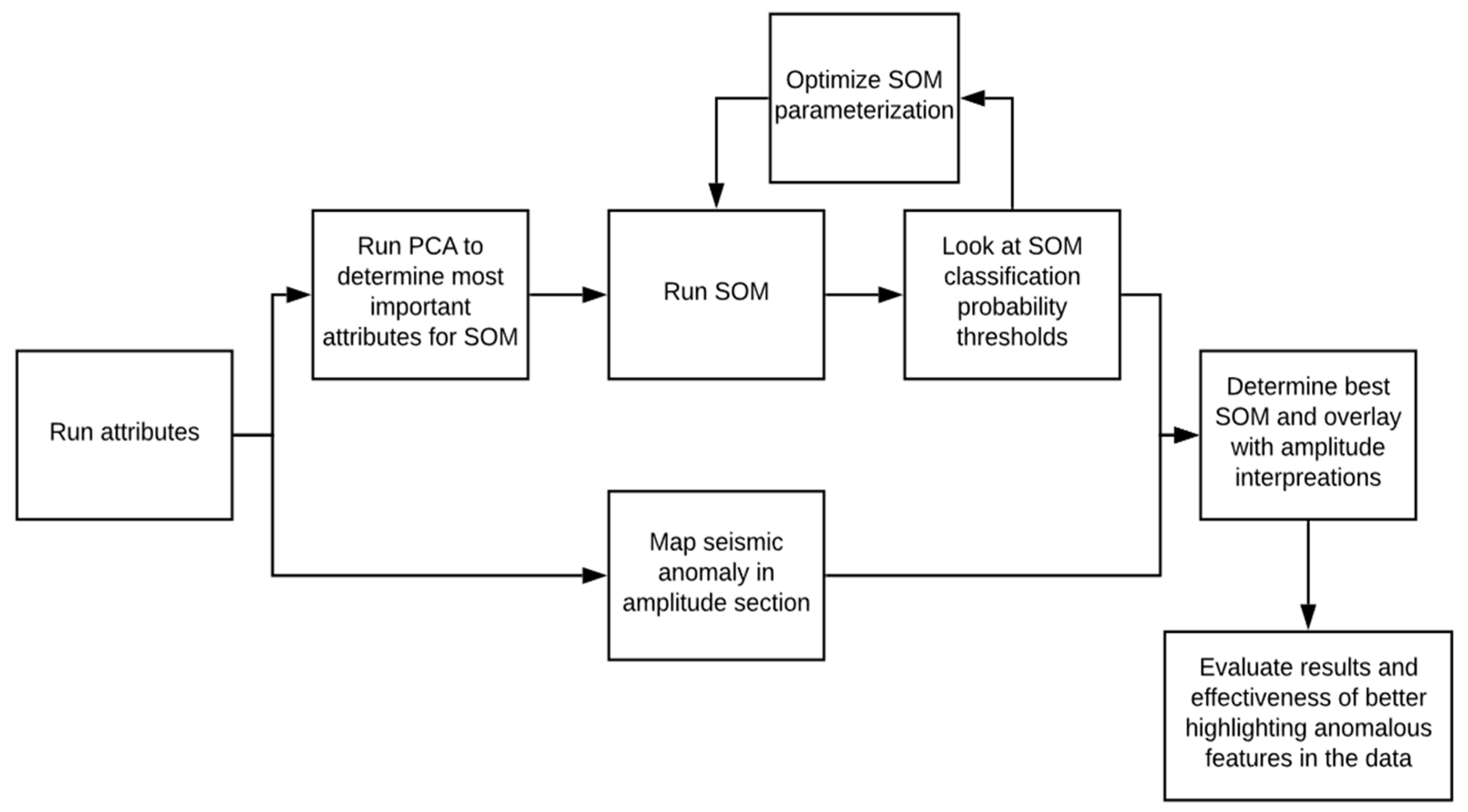
3.2. Methods and Workflow

Potential gas prospects have been traditionally identified through the use of seismic reflection data with certain types of seismic amplitude anomalies referred to as Direct Hydrocarbon Indicators (DHIs) [18]. Dozens of recognized DHIs exist, and they vary depending on particulars of each basin—such as depth, rock type, and fluid type pressure. Gas presence in Tertiary Gulf of Mexico rocks is identified as a DHI AVO class 3 that displays a larger amplitude response in the far angles compared to the near angles [19,20]. In full-stack seismic, the gas is highlighted as a bright spot [18]. Additionally, a velocity-sag anomaly is occasionally observed in seismic time volumes beneath large accumulations, where the seismic reflectors appear to be pulled down with increasing time due to the presence of lower velocity gas [18]. Although these seismic DHIs point to the presence of gas, they cannot quantify gas saturation to a degree where the economic validity of the reservoir can be reliably determined. DHIs are only indicators that hydrocarbons could be present, and thus, are vulnerable to uncertainty. This low-saturation gas phenomenon is pervasive, occurring in hydrocarbon basins globally from the Gulf of Mexico, to the North Sea, and the Niger Delta [2,3,13,21,22].
Despite decades of research from primarily the rock physics discipline, minimal improvement in identifying gas saturation variations from seismic data has been achieved [3,5,6,7,23,24]. A robust method of identifying and discriminating potential LSG occurrences remains unsolved, resulting in an additional factor in hydrocarbon exploration risk. Furthermore, even with well logs available, gas saturations may be unclear. Therefore, a new methodology is proposed, which uses unsupervised machine learning multi-attribute analysis on 3D, post-stack seismic data with principal component analysis (PCA) and self-organizing maps (SOMs). This study used Paradise Version 3.1, a commercial tool provided by Geophysical Insights, to conduct our PCA and SOM investigations. This methodology is outlined in Figure 6 and shows promise for de-risking prospects, even if it is not quantitative. This method can be particularly helpful in frontier and exploration basins where wells may not exist or be very limited.
The initial analysis used PCA methods applied to a set of seismic attributes from the 3D post-stack seismic survey within the Green Canyon, Gulf of Mexico. PCA is a linear mathematical technique that reduces a set of variables, such as seismic attributes, to a set that illustrates the majority of the independent information. variation [25,26]. Therefore, PCA will aid in identifying meaningful combinations of attributes that better delineate between low-saturation and high-saturation gas reservoirs. This method has been applied to a myriad of geophysical applications [8,9,12,27,28]. The first principal component accounts for the most variability in the data with each succeeding orthogonal component accounting for the remaining variability. Although the first principal component highlights the largest linear attribute combinations that best represent the variability of the bulk of the data, it may not identify specific features of interest to the interpreter. Therefore, succeeding principal components were evaluated because they may be associated with low-saturation gas characteristics that were not identified with the first principal component. Additionally, many attributes that are useful for characterizing high-amplitude anomalies, such as attributes sensitive acoustic impedance changes, were pre-selected to be used within the PCA. Nonetheless, PCA will reduce these seismic attributes down to a smaller subset that is representative of most of the data’s independent variability.
Following PCA analysis, the attributes deemed the most successful for differentiating between different levels of gas saturation are then incorporated into a SOM. Due to the multidimensional nature of PCA results, SOMs are employed to help visualize these complex relationships [28]. Once the SOM model is optimized for KK/LA prospects within the Green Canyon Phase II survey, the same model will then be applied to the Ursa (Shell Mississippi Canyon 3D seismic survey) and Scarborough (Scarborough 3D seismic survey) fields to evaluate its effectiveness for differentiating between high and low saturation gas reservoirs.
A SOM is a collection of neurons that classify data samples into categories based on their various geological or geophysical properties. For a successful analysis, it is critical to properly configure the SOM initialization hyperparameters. Therefore, several SOM hyperparameters, such as the number of neurons and epochs, were evaluated to determine optimal parameterization. We resumed the methodologies established by Roden et al. [8,9,12] for investigating seismic data where they provide suggestions for optimizing SOM hyperparameters. The SOM was run on a 5 × 5 neuron count (total of 25 neurons) with 100 epochs (iterations) over the entire 3D seismic volume. These neuron dimensions and number of epochs were used because they are robust enough to highlight minute changes and details within the seismic data, such as varying gas saturations, while also being computationally efficient. Our initialization parameters were similar to those proposed by Roden et al. [8] as well as Roden and Santogrossi [29]. Roden et al. [8] recommend 60–100 epochs of training when applying SOMs to interpret seismic data. Both papers also found that a 5 × 5 neuron count was ideal for identifying DHIs [8,29]. We built upon their methodologies and evaluated how different neuron counts would affect our SOM results. Further exploratory data analysis revealed that neuron dimensions higher than 5 × 5 tended to classify noise within individual neurons and display insignificant information. Neuron dimensions lower than 5 × 5 were insufficient for extracting meaningful information about varying gas saturation. Finally, to visualize and interpret SOM results, the neurons are nonlinearly mapped to a 2D colormap that preserves the topological ordering of the input space [8,9,29,30]. Interpreters can then identify and visualize the location of the neurons in the 3D survey [8,9,29,30]. The color of each neuron can be modified on the Paradise’s interactive 2D colormap to better reveal geological features within the dataset [8,9,29]. Further detailed explanations of the SOM neuron classification and visualization processes for the Paradise tool can be found in Roden et al. [8], Roden and Santogrossi [29], as well as Smith and Treitel [30].
Inlines (IL) containing noticeable gas saturations, such as IL 2391 (shown in Figure 3), showed highly anomalous eigenvalues from the PCA results compared to other lines in the survey (Figure 7). These anomalous eigenvalue responses are most likely attributed to the anomalous amplitude responses present within that line. Further analysis of these anomalous lines revealed that instantaneous attributes that identify changes in amplitude, frequency, and phase tended to cluster together to reveal highly anomalous areas within the seismic. For example, the sweetness and envelope seismic attributes ranked as the highest attributes within the second eigenvector for IL 2391 (Figure 7). In Figure 7, “Percentage” represents the degree to which the attribute contributed towards that specific eigenvector whereas “Percent Total” lists the variance for each of the attributes from all the eigenvectors. Sweetness and envelope appeared to contribute the most towards the second eigenvector while also representing 62.00% and 58.04% of the variance for all the eigenvectors. This signifies that those two attributes captured a significant amount of the variability within the dataset. Following a similar workflow used for the second eigenvector, the highest-ranking attributes from the first few eigenvectors were chosen to be incorporated into the SOM analysis over the entire dataset. These attributes are the full-stack amplitude, envelope, Hilbert, cosine of instantaneous phase, relative acoustic impedance, and sweetness.

4. Results

Once the SOM hyperparameters were optimized, this study then evaluated the number of attributes to use within the SOM model. This was determined through iterative PCA and SOM analysis. The optimized SOM model used the following instantaneous attributes: full-stack amplitude, envelope, Hilbert, cosine of instantaneous phase, relative acoustic impedance, and sweetness. These attributes for the KK/LA SOM are shown in Figure 8A–F, and Table 1 describes the definitions and uses of these attributes.

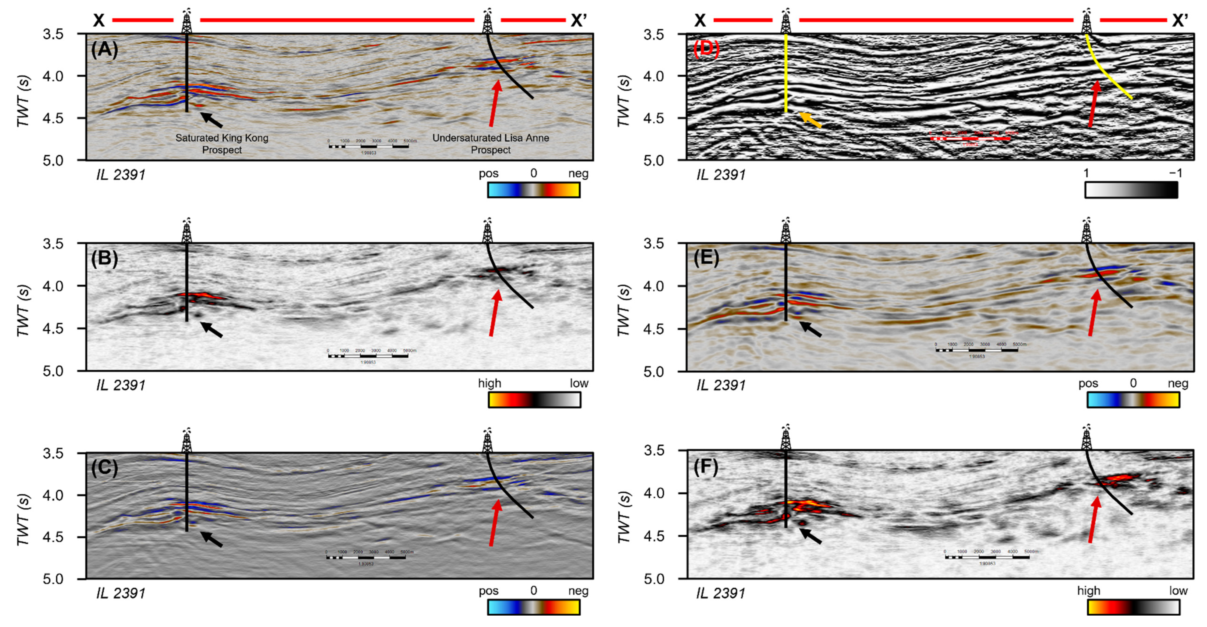
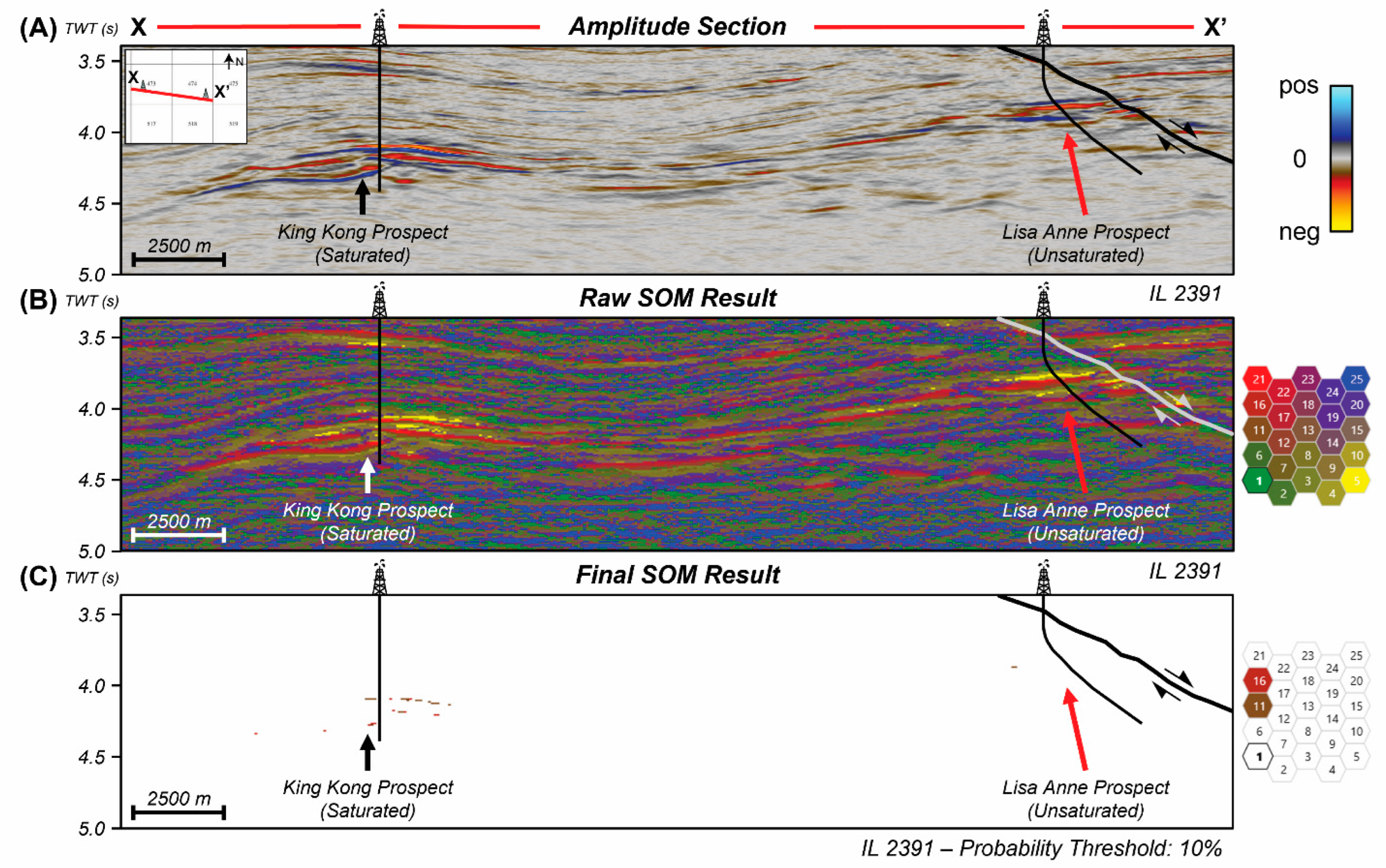
4.1. KK/LA SOM Results

The goal of the multi-attribute analysis is to qualitatively attempt to distinguish between high- and low-saturation gas reservoirs. The undersaturated Lisa Anne prospect exhibits a similar amplitude and seismic attribute response to the one observed for the higher-saturated King Kong prospect (Figure 8A–F). However, when using an unsupervised, multi-attribute analysis, the King Kong prospect can be isolated from the undersaturated Lisa Anne prospect (Figure 9A–C). Figure 9A highlights two very bright amplitude anomalies known as the KK/LA prospects, whereas Figure 9B shows the raw SOM result for the same line with all of the neurons highlighted. Figure 9C displays the SOM results displayed with the anomalous neurons of interest (Neurons 11 and 16).
These neurons are showing the data points which had a probability threshold of less than 10%, meaning that the data points are filtered to show those that only have a 0–10% chance of being classified within those clusters. By using this probability cutoff, the SOM is displaying the highly anomalous data points that had a 10% chance of being grouped within that neuron. Therefore, these anomalous data points are displaying anomalous amplitude responses. Other neurons grouped noise or different geologic features such as bedding and other lithology variations. In Figure 9C, the top and base of the King Kong prospect are well defined, with the Lisa Anne prospect effectively suppressed and undefined. A 3D analysis revealed that the SOM results continuously follow the amplitude anomalies observed in the seismic data. This continues throughout the two reservoir intervals, with the King Kong reservoir extent clearly defined, and the Lisa Anne extents remaining indiscernible (Figure 9C).

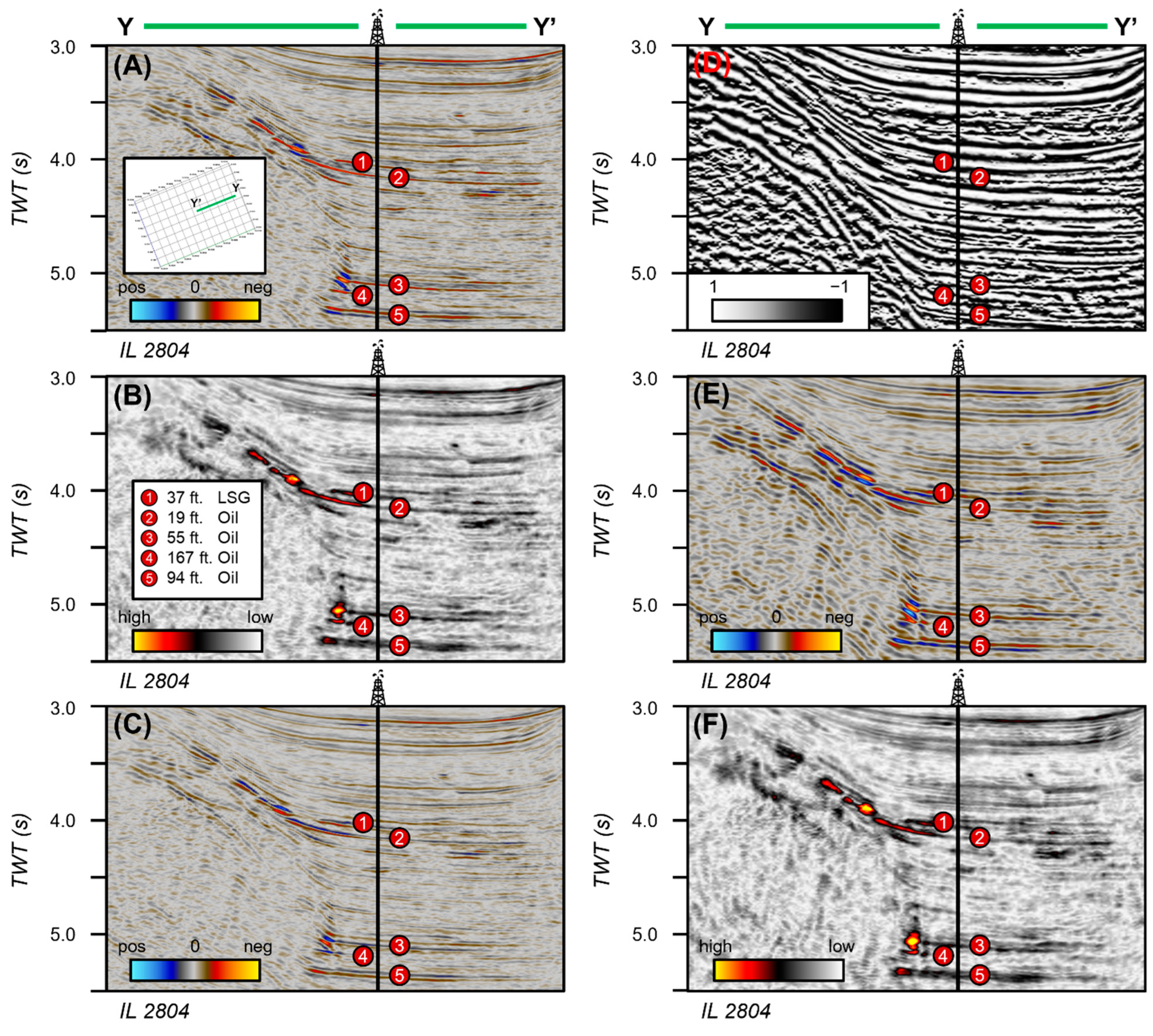
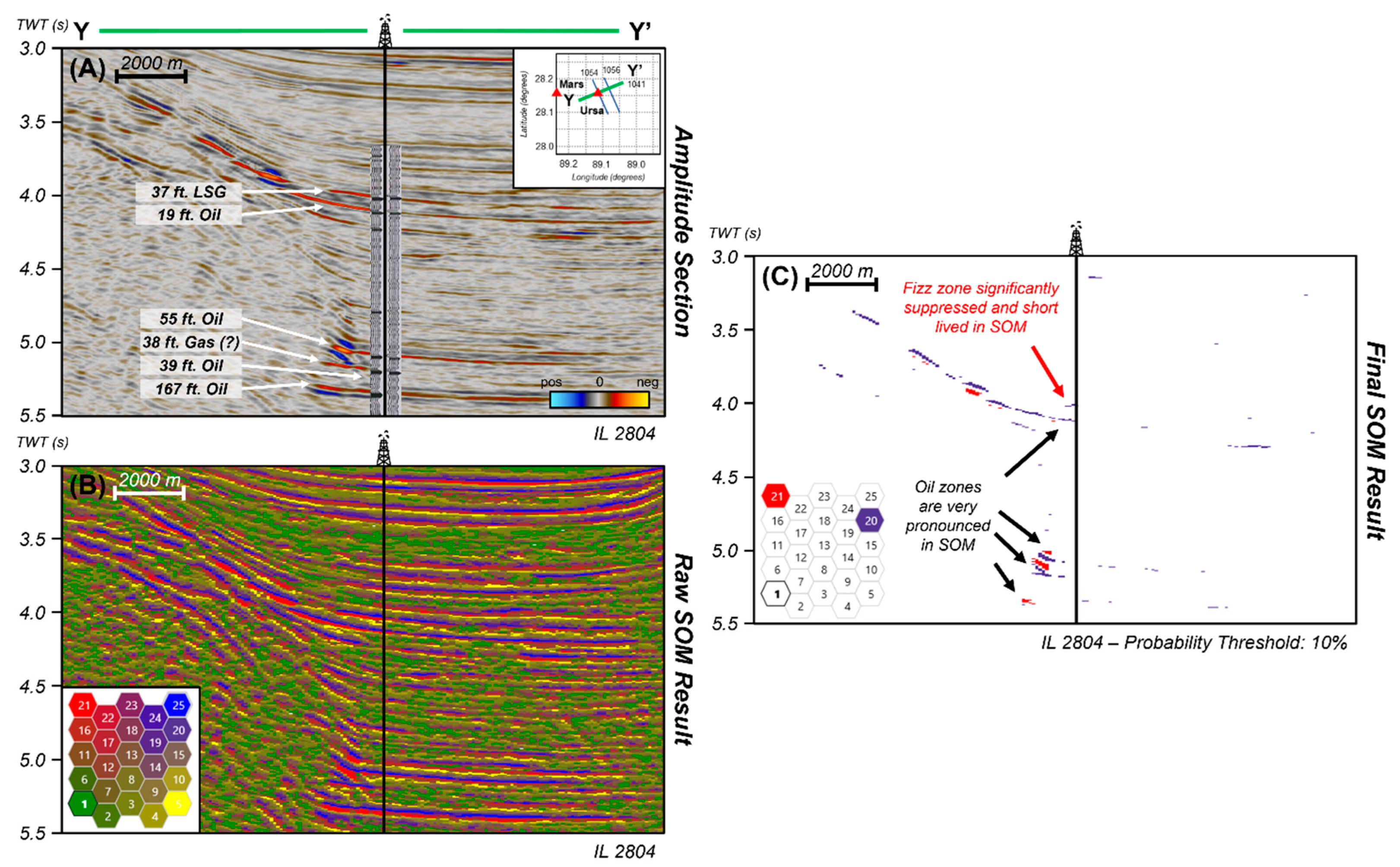
4.2. Ursa SOM Results

The KK/LA SOM model was then applied to the Shell Mississippi Canyon 3D seismic survey over the Ursa gas field, offshore of the Gulf of Mexico. We used the same seismic attributes that were used in the KK/LA SOM. The attributes for the Ursa SOM are shown in Figure 10A–F. Well log and AVO analysis from Hilterman [2] revealed that one of the upper reservoir intervals was an LSG interval (Figure 4 and Figure 10A). In Figure 10A–F, the LSG interval is marked by Circle 1, whereas the productive hydrocarbon intervals are marked by Circles 2–5. Looking at all the attribute responses in Figure 10A–F, the LSG interval demonstrates a similar response to the higher hydrocarbon-saturated reservoirs in the lower intervals.
However, once all the attributes are combined using the SOM, the LSG interval becomes significantly smaller and less continuous compared to the higher saturated hydrocarbon intervals (Figure 11A–C). The LSG interval appears significantly more continuous in the amplitude section of Figure 11A and the raw SOM section with all the neurons highlighted, whereas it is less apparent and discontinuous in Figure 11C. Figure 11C is the same SOM from Figure 11B with only the neurons of interest displayed with a probability threshold of 10% applied. The prolific hydrocarbon intervals below the LSG interval appear to be more continuous in the SOM result observed in Figure 11C. However, the LSG interval is still somewhat apparent in the Ursa SOM, whereas the LSG interval is almost indiscernible in the KK/LA SOM (Figure 9B).

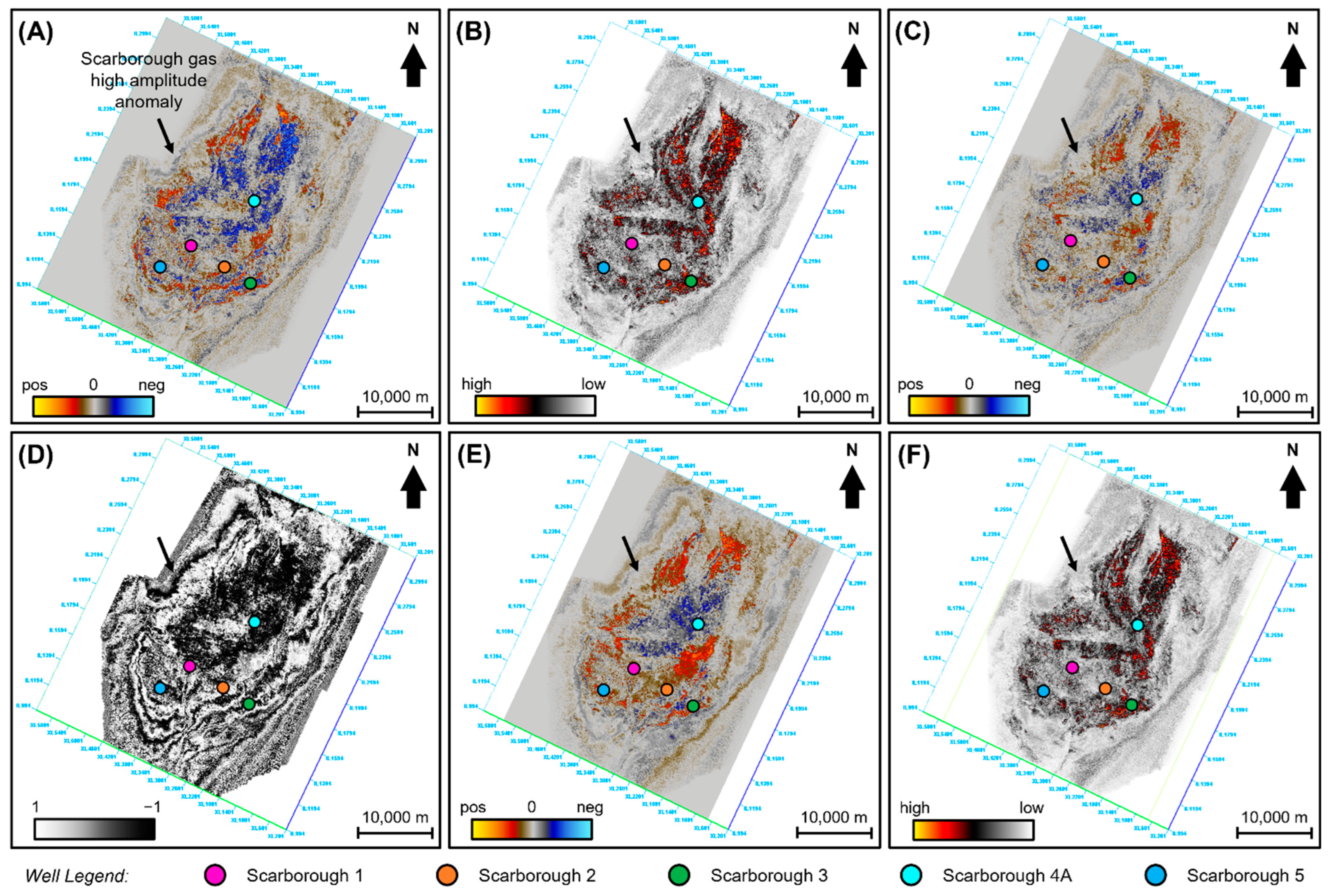
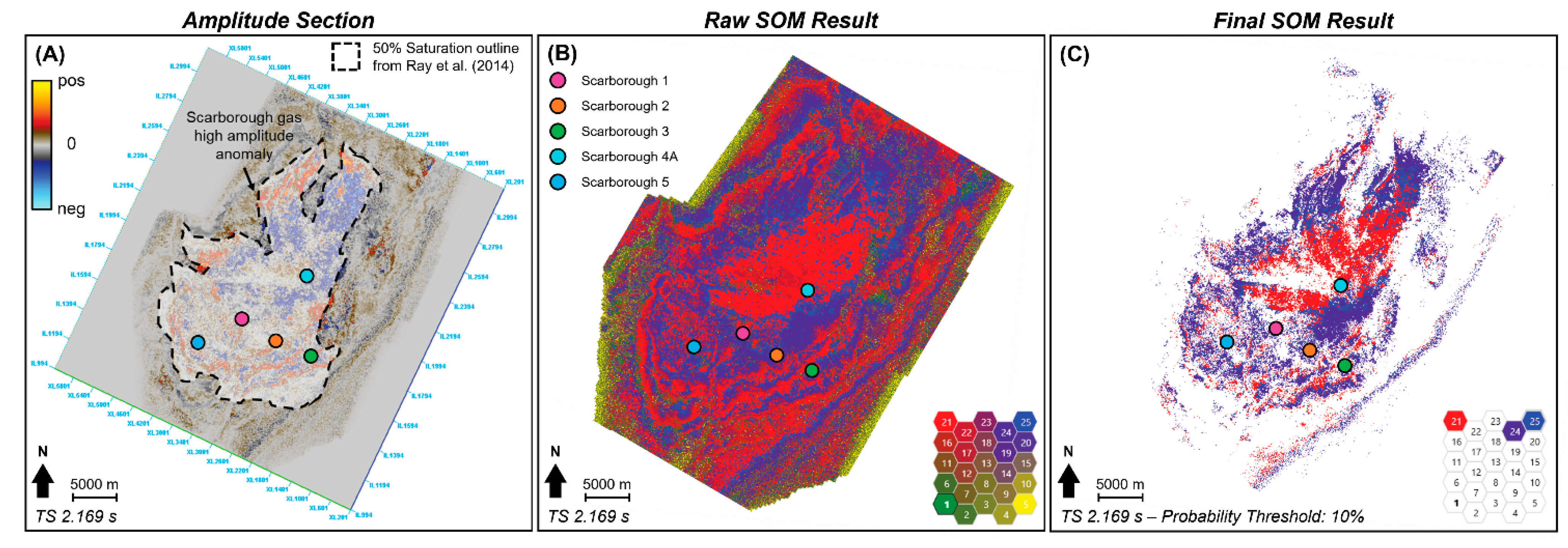
4.3. Scarborough SOM Results

Once the SOM was successfully applied to the KK/LA prospects and to the Ursa gas field, the model was then applied to the Scarborough gas field, offshore Australia. The same seismic attributes from the KK/LA and Ursa SOM are shown for the Scarborough gas interval in Figure 12A–F. The seismic attributes taken over the Scarborough gas interval exhibit similar responses to one another, where the individual attributes provide no indication of varying gas saturation levels (Figure 12A–F). However, once the individual attributes are incorporated together into a SOM, the saturation of the Scarborough gas field can be better characterized (Figure 13A–C). A study by Ray et al. [4] characterized the areal extent of the Scarborough reservoir by applying a Bayesian inversion on controlled source electromagnetic (CSEM) data from five exploration wells and available 3D seismic coverage (Figure 5B). From their synthetic studies, they were able to map the outline of the Scarborough reservoir where gas saturation was higher than 50%. The Scarborough SOM result, with a probability threshold of 10% applied, appears to match quite well with the saturation outline proposed by Ray et al. [4] (Figure 13C).

5. Discussion

Taking a closer look at individual neuron weights from the SOMs, some attributes appear to represent the entire variability of the dataset, while other attributes appear to contribute towards the individual neuron’s ability to represent the amplitude anomalies (Figure 14A–C). Overall, the clustering results from the KK/LA SOM reveal that the instantaneous envelope had a total independence of 35.2%, followed by sweetness at 33.9% and relative acoustic impedance at 12.9% (Figure 14A). Total independence represents the weight that the attributes play during clustering over the entire dataset. Therefore, these three attributes clustered 82.0% of the data with the remaining attributes, such as the cosine of instantaneous phase, the Hilbert, and the full-stack amplitude, further delineating these clusters to differentiate between low- and high-saturation gas reservoirs (Figure 14A). Notice that while these three attributes represented 82.0% of the dataset, they were not always the most prominent within Neurons 11 and 16. Attributes such as the Hilbert contributed nearly 30% towards Neuron 16, whereas it only represented 11.4% of KK/LA’s independent variability (Figure 14A). Therefore, the Hilbert attribute played a significant role in classifying the anomalous amplitude responses in the KK/LA SOM. A similar relationship is also observed within the Ursa SOM, where the instantaneous envelope, sweetness, and relative acoustic impedance represented 60% of the data’s variance compared to the cosine of instantaneous phase, the Hilbert, and the full-stack amplitude, which represented the remaining 40% (Figure 14B). Yet, these three attributes did not always have the highest neuron independence. Notice how the Hilbert in Neuron 20 of the Ursa SOM contributed over 25% towards that cluster, whereas it only represented 14.3% of Ursa’s independent variability (Figure 14B). This same observation was also noted within Neurons 11 and 16 in the KK/LA survey (Figure 14A).
However, when looking at the Scarborough SOM clustering results, an opposite relationship is observed from the KK/LA and Ursa SOMs (Figure 14C). Seismic attributes such as the cosine of instantaneous phase, the full-stack amplitude, and relative acoustic impedance now represent approximately 85.7% of the independent data’s variability when this relationship was the inverse in the KK/LA and Ursa SOMs (Figure 14C). Yet these attributes consistently contributed the most towards classifying anomalous amplitudes in Neurons 21, 24, and 25 while the other attributes complimented the classification (Figure 14C). In fact, now we observe that attributes such as sweetness and the instantaneous envelope represented 0% of the independent data’s variability and played a minor role in the individual neuron classifications. These null values indicate that the KK/LA and Ursa SOMs are not properly optimized for the Scarborough gas field (Figure 14A–C). These SOM differences could be attributed to different amplitude responses from two different basins, meaning that the amplitude responses in the Gulf of Mexico are different than the amplitudes in the Scarborough gas field. These differences could be due to different burial histories and pressure regimes [20,38]. They could also be due to differences in fluid saturations, such as gas and brine [23,38]. Based on these results, the SOM models are only optimized for within the Gulf of Mexico, as was noted within the KK/LA and Ursa fields (Figure 9C and Figure 11C), whereas a new combination of attributes is required for the Carnarvon Basin, as was observed within Scarborough SOM (Figure 13C). Additionally, it is important to note that these SOMs all used a probability threshold of 10% to better represent the anomalous data points within the neurons. Therefore, these neurons are highlighting the data points that only had a 0–10% chance of being classified within those clusters. This probability threshold of the model further enhances the visualization capabilities for the interpreter as it allows them to better capture the highly anomalous responses within the data, which are not necessarily easily visualized through seismic amplitude and attribute profiles.
Studies by Taner [31,33] and Chopra and Marfurt [32] noted that the instantaneous envelope is useful for highlighting lithology, porosity, and hydrocarbons since the attribute is sensitive to subtle changes in acoustic impedance. Additionally, the instantaneous envelope attribute is derived using the Hilbert transform to illustrate the signal’s instantaneous energy, which means that it is also using the complex portion of the seismic trace [31,32]. Therefore, this attribute could be effective for capturing the subtle amplitude differences between low and high-saturation gas reservoirs within both the real and imaginary seismic trace. When the instantaneous envelope is used in combination with other attributes that are good for identifying DHIs, such as sweetness and relative acoustic impedance, the SOM can qualitatively differentiate between high and low gas saturations in the KK/LA and Ursa fields (Figure 9A–C and Figure 11A–C). Additionally, attributes such as Hilbert and the cosine of instantaneous phase that are useful for analyzing AVO anomalies and highlighting bed continuity, respectively, could be further complimented by the other attributes to better classify the anomalous amplitude responses within the SOM [31,32]. However, this method proved to be limited in the Scarborough gas field as the results yielded limited qualitative information about reservoir saturation (Figure 14A–C). Yet, the Scarborough SOM did manage to highlight the amplitude anomaly created by the gas fairly well. More work is needed to optimize the SOM model for the Scarborough gas field.
A recent study by Batzle [13] conducted a detailed, 3D reservoir model using fluid substitution to better characterize the Ursa LSG interval. The report found that the Ursa LSG zone may have a higher saturation than was originally thought and could be a commercial hydrocarbon zone [13]. Therefore, this could be a reason why the Ursa LSG zone is still visible in the SOM results, albeit significantly less continuous than the other hydrocarbon intervals. Future work will involve obtaining well data, such as sonic logs, to better characterize the hydrocarbon intervals. Furthermore, a closer comparison between the amplitude section and the SOM result reveals that they are quite similar to one another and map similar extents (Figure 13A–C). Therefore, it appears that the SOM model is limited to better characterizing relative saturations between reservoirs in the same seismic survey. Future work will involve better characterization of the Scarborough gas interval to determine if there are higher saturation locations within the reservoir that would be optimal for further production.
Finally, another important note to consider for LSG is the detailed consideration of containment. Most LSG is in a sprung trap—a gas accumulation that leaked from seal failure and residual gas remains (5% to 25% gas saturation) [2,3,16,22]. O’Brien [3] noted that hydrocarbon leakage up the regional fault normal fault may have been possible for the Lisa Anne prospect. He observed shallow bright spots due to gas pockets and water bottom coring [3]. While this does decrease the risk of hydrocarbon migration, it does suggest an increased risk of containment [3]. Furthermore, while Hilterman [2] did not discuss seal integrity in detail, Wojcik et al. [22] note the importance of incorporating seal risk analysis within other turbidite reservoirs within the Gulf of Mexico. Finally, Foschi and Cartwright [16] observed seal failure within the Scarborough gas field and characterized a 100 km2 (38 mi2) wide leakage zone with more than 500 pockmarks. This suggests that there could be some LSG-prone regions within the field. However, many of the wells within the field have considerably large gas saturations [14]. When looking at the SOM results, this is not readily apparent, especially in the case of the unoptimized Scarborough SOM result (Figure 9C, Figure 11C and Figure 13C). However, seal failure analysis has shown promising results for further characterization of LSG reservoirs, and future work would incorporate a detailed seal analysis of the discussed reservoirs [7,16,22].

6. Conclusions

Preliminary results suggest that instantaneous attributes that detect changes in the amplitude, frequency, and phase tend to cluster together in the PCA to reveal highly anomalous areas within the seismic. SOM results highlighted the top and base of the King Kong prospect while the Lisa Anne LSG prospect remained undetected, showing that there is a noticeable difference between both prospects (Figure 9C). Upon applying the KK/LA SOM to the Ursa gas field, the SOM showed that the Ursa LSG interval became significantly suppressed and less continuous compared to the higher saturated hydrocarbon intervals present within the lower intervals (Figure 11C). Although the Ursa LSG interval is still apparent in the SOM, whereas it was almost indiscernible in the KK/SOM, a study by Batzle [13] found that the LSG zone may have a higher saturation than was originally thought and could be a commercial hydrocarbon zone. Although these results may not give a definitive saturation result, they do highlight a stark difference between both prospects.
However, it appears that the method is limited to only differentiating between relative hydrocarbon saturations within the same seismic survey. Upon further analyzing the neuron clusters, attributes such as the instantaneous envelope and sweetness represent 0% of the independent data within the Scarborough SOM (Figure 14A–C). This suggests that the combination of attributes is unoptimized for the Scarborough SOM. This is most likely due to the Scarborough gas fields having a different amplitude response resulting from a different burial history and fluid saturations when compared to the Gulf of Mexico [20,38].
In the instance of neighboring prospects (as was the case with the KK/LA prospects) or stacked reservoir systems (such as the Ursa gas field), these results can further be incorporated into hydrocarbon exploration risking to better understand DHIs in the subsurface and prevent uneconomic wells from being drilled. Individually, some of these attributes have no success in differentiating between high and low saturation gas prospects. However, employing a multi-attribute analysis provides clearer insight and more confidence in delineating between high and low saturation gas reservoirs. Although not currently available, supplementary research will incorporate seismic gathers, angle stacks, and well data into this method to further improve results.

Author Contributions

Conceptualization, J.C. and H.B.; Data curation, J.C. and H.B.; Formal analysis, J.C.; Methodology, J.C. and H.B.; Project administration, J.C. and H.B.; Software, J.C.; Supervision, H.B.; Writing—original draft, J.C.; Writing—review and editing, J.C. and H.B. All authors have read and agreed to the published version of the manuscript.

Funding

This research was funded by initial startup funds from the University of Oklahoma and from AASPI (Attribute Assisted Seismic Processing and Interpretation).

Data Availability Statement

USGS National Archive of Marine Seismic Surveys (NAMSS) and the Bureau for Ocean Energy Management (BOEM) for access to the Green Canyon Phase II 3D seismic survey (G3D201407-02), the Shell Mississippi Canyon 3D seismic survey (G3D1304-002A through C), as well as the protraction grid and seafloor outlines. We would like to also thank the Australian Government for providing open access to the Scarborough 3D seismic survey.

Acknowledgments

We would like to acknowledge USGS National Archive of Marine Seismic Surveys (NAMSS) and the Bureau for Ocean Energy Management (BOEM) for access to the Green Canyon Phase II 3D seismic survey (G3D201407-02), the Shell Mississippi Canyon 3D seismic survey (G3D1304-002A through C), as well as the protraction grid and seafloor outlines. We would like to also thank the Australian Government for providing open access to the Scarborough 3D seismic survey. The authors would like to give additional thank you to Geophysical Insights, Schlumberger, and ESRI for software license donations to the University of Oklahoma. We would like to also thank AASPI (Attribute-Assisted Seismic Processing and Interpretation) consortium for their software package and the SDA (Subsurface Detective Agency) consortium for their much-appreciated feedback. Finally, thank you to Mike Forrest and Rocky Roden for their valuable insights and recommendations for improving this manuscript.

Conflicts of Interest

The authors declare that they have no conflict of interest.

References

  1. Zhao, B.; Zhou, H.; Hilterman, F.J. Fizz and gas separation with SVM classification. In Proceedings of the SEG Annual Meeting, Houston, TX, USA, 6–11 November 2005. [Google Scholar] [CrossRef]
  2. Hilterman, F.J. Seismic Amplitude Interpretation; Society of Exploration Geophysicists: Houten, The Netherlands; European Association of Geoscientists and Engineers: Houten, The Netherlands, 2001. [Google Scholar] [CrossRef]
  3. O’Brien, J. Seismic amplitudes from low gas saturation sands. Lead. Edge 2004, 23, 1236–1243. [Google Scholar] [CrossRef]
  4. Ray, A.; Key, K.; Bodin, T.; Myer, D.; Constable, S. Bayesian inversion of marine CSEM data from the Scarborough gas field using a transdimensional 2-D parametrization. Geophys. J. Int. 2014, 199, 1847–1860. [Google Scholar] [CrossRef] [Green Version]
  5. Zhu, F. Shear-Wave Velocity Estimation Using Multiple Logs and Multicomponent Seismic AVO Interpretation: Gulf of Thailand. Ph.D. Thesis, Texas A&M University, College Station, TX, USA, 2010. [Google Scholar]
  6. Zhou, Z.; Hilterman, F.J. A comparison between methods that discriminate fluid content in unconsolidated sandstone reservoirs. Geophysics 2010, 75, B47–B58. [Google Scholar] [CrossRef]
  7. Laiw, A. Low Saturation Gas Reservoirs Discrimination—An Integrated Approach. In Proceedings of the 73rd EAGE Conference and Exhibition, Vienna, Austria, 23–27 May 2011. [Google Scholar] [CrossRef]
  8. Roden, R.; Smith, T.; Sacrey, D. Geologic pattern recognition from seismic attributes: Principal component analysis and self-organizing maps. Interpretation 2015, 3, SAE59–SAE83. [Google Scholar] [CrossRef]
  9. Roden, R.; Chen, C.W. Interpretation of DHI characteristics with machine learning. First Break 2017, 35. [Google Scholar] [CrossRef]
  10. Sacrey, D.; Roden, R. Solving exploration problems with machine learning. First Break 2018, 67–72. [Google Scholar] [CrossRef]
  11. Chopra, S.; Marfurt, K.J. Unsupervised machine learning applications for seismic facies classification. In Proceedings of the Unconventional Resources Technology Conference, Denver, CO, USA, 22–24 July 2019; pp. 3135–3142. [Google Scholar] [CrossRef]
  12. Roden, R.; Smith, T.A.; Santogrossi, P.; Sacrey, D.; Jones, G. Seismic interpretation below tuning with multiattribute analysis. Lead. Edge 2017, 36, 330–339. [Google Scholar] [CrossRef]
  13. Batzle, M. Seismic Evaluation of Hydrocarbon Saturation in Deep-Water Reservoirs; Colorado School of Mines: Golden, CO, USA, 2016. [Google Scholar] [CrossRef]
  14. Han, C. Understanding frequency decomposition colour blends using forward modelling—Examples from the Scarborough gas field. First Break 2018, 36, 53–60. [Google Scholar] [CrossRef]
  15. Driscoll, N.W.; Karner, G.D. Lower crustal extension across the Northern Carnarvon basin, Australia: Evidence for an eastward dipping detachment. J. Geophys. Res. Solid Earth 1998, 103, 4975–4991. [Google Scholar] [CrossRef]
  16. Foschi, M.; Cartwright, J.A. Seal failure assessment of a major gas field via integration of seal properties and leakage phenomena. AAPG Bull. 2020, 104, 1627–1648. [Google Scholar] [CrossRef]
  17. Glenton, P.N.; Sutton, J.T.; McPherson, J.G.; Fittall, M.E.; Moore, M.A.; Heavysege, R.G.; Box, D. Hierarchical approach to facies and property distribution in a basin-floor fan model, Scarborough Gas Field, North West Shelf, Australia. In Proceedings of the IPTC 2013: International Petroleum Technology Conference, Beijing, China, 26–28 March 2013; p. cp-350. [Google Scholar] [CrossRef]
  18. Brown, A.R. Interpretation of Three-Dimensional Seismic Data; Society of Exploration Geophysicists: Tulsa, OK, USA; American Association of Petroleum Geologists: Tulsa, OK, USA, 2011. [Google Scholar] [CrossRef] [Green Version]
  19. Castagna, J.P.; Backus, M.M. Offset-Dependent Reflectivity—Theory and Practice of AVO Analysis; Society of Exploration Geophysicists: Houston, TX, USA, 1993. [Google Scholar] [CrossRef]
  20. Chopra, S.; Castagna, J.P. AVO; Society of Exploration Geophysicists: Houston, TX, USA, 2014. [Google Scholar] [CrossRef]
  21. Khalid, P.; Ghazi, S. Discrimination of fizz water and gas reservoir by AVO analysis: A modified approach. Acta Geod. Geophys. 2013, 48, 347–361. [Google Scholar] [CrossRef]
  22. Wojcik, K.M.; Gonzalez, E.; Vines, R.E. Derisking low-saturation gas in Tertiary turbidite reservoirs. Interpretation 2016, 4, SN31–SN43. [Google Scholar] [CrossRef]
  23. Han, D.H.; Batzle, M. Fizz water and low gas-saturated reservoirs. Lead. Edge 2002, 21, 395–398. [Google Scholar] [CrossRef]
  24. Wu, X.; Chapman, M.; Li, X.Y.; Boston, P. Quantitative gas saturation estimation by frequency-dependent amplitude-versus-offset analysis. Geophys. Prospect. 2014, 62, 1224–1237. [Google Scholar] [CrossRef] [Green Version]
  25. Jolliffe, I.T. Mathematical and statistical properties of population principal components. Princ. Compon. Anal. 2002, 10–28. [Google Scholar] [CrossRef]
  26. Sacrey, D.; Roden, R. Understanding Attributes and Their Use in the Application of Neural Analysis–Case Histories Both Conventional and Unconventional. Search Discov. Artic. 2014, 41473. [Google Scholar]
  27. La Marca, K.; Bedle, H. Deepwater seismic facies and architectural element interpretation aided with unsupervised machine learning techniques: Taranaki basin, New Zealand. Mar. Pet. Geol. 2022, 136. [Google Scholar] [CrossRef]
  28. Kohonen, T. The self-organizing map. Proc. IEEE 1990, 78, 1464–1480. [Google Scholar] [CrossRef]
  29. Roden, R.; Santogrossi, P. Significant advancements in seismic reservoir characterization with machine learning. First–SPE Nor. Mag. 2017, 3, 14–19. [Google Scholar]
  30. Smith, T.; Treitel, S. Self-organizing artificial neural nets for automatic anomaly identification. In SEG Technical Program Expanded Abstracts; Society of Exploration Geophysicists: Houston, TX, USA, 2010; pp. 1403–1407. [Google Scholar]
  31. Taner, M.T.; Koehler, F.; Sheriff, R.E. Complex seismic trace analysis. Geophysics 1979, 44, 1041–1063. [Google Scholar] [CrossRef]
  32. Chopra, S.; Marfurt, K.J. Seismic attributes—A historical perspective. Geophysics 2015, 70, 3SO–28SO. [Google Scholar] [CrossRef]
  33. Taner, M.T. Seismic attributes. Can. Soc. Explor. Geophys. Rec. 2001, 26, 49–56. [Google Scholar]
  34. Subrahmanyam, D.; Rao, P.H. Seismic attributes—A review. In Proceedings of the 7th International Conference & Exposition on Petroleum Geophysics, Hyderabad, India, 16–19 September 2008; pp. 398–404. [Google Scholar]
  35. Radovich, B.J.; Oliveros, R.B. 3-D sequence interpretation of seismic instantaneous attributes from the Gorgon field. Lead. Edge 1998, 17, 1286–1293. [Google Scholar] [CrossRef]
  36. Hart, B. Channel detection in 3-D seismic data using sweetness. AAPG Bull. 2008, 92, 733–742. [Google Scholar] [CrossRef]
  37. Koson, S.; Chenrai, P.; Choowong, M. Seismic attributes and their applications in seismic geomorphology. Bull. Earth Sci. Thail. 2013, 6, 1–9. [Google Scholar]
  38. Avseth, P.; Flesche, H.; Van Wijngaarden, A.J. AVO classification of lithology and pore fluids constrained by rock physics depth trends. Lead. Edge 2003, 22, 1004–1011. [Google Scholar] [CrossRef]
Figure 1. Change in rock properties with increasing gas saturation. The bulk modulus quickly decreases with a relatively small amount of gas saturation. This bulk modulus similarity between low- and high-gas saturation is the crux of the LSG gas differentiation problem.
Geosciences 12 00132 g001
Figure 2. Location of the 3D seismic surveys used in this study. Two of these datasets are located in (A) offshore Gulf of Mexico, while the other dataset is located in (B) offshore Australia within the Northern Carnarvon Basin. Gulf of Mexico protraction grid and seafloor outlines taken from the BOEM.
Geosciences 12 00132 g002
Figure 3. Inline 2391 taken through the KK/LA 3D seismic survey across the King Kong and Lisa Anne wells over Green Canyon Block 473 and 474, offshore Gulf of Mexico (modified from O’Brien [3]).
Geosciences 12 00132 g003
Figure 4. Inline 2804 taken through the Ursa Field 3D seismic survey. The hydrocarbon intervals and a synthetic from Hilterman, 2001 are highlighted on the seismic section. Notice how the amplitude for the LSG interval exhibits a similar response to the other hydrocarbon producing intervals (modified after Hilterman [2]).
Geosciences 12 00132 g004
Figure 5. (A) A horizontal time slice taken at 2.169 s through the Scarborough seismic survey displaying the high amplitude anomaly of the Scarborough gas field. (B) A CSEM study by Ray et al. [4] where they defined the 50% gas saturation outline within the Scarborough gas field (modified after Ray et al. [4]). (C) Interpreted arbitrary seismic section highlighting the Scarborough gas anomalies, key horizons, and wells used for this study.
Geosciences 12 00132 g005
Figure 6. Iterative SOM workflow used to evaluate the accuracy and effectiveness of each SOM result. Several combinations of instantaneous attributes and SOM parameters were evaluated in this study.
Geosciences 12 00132 g006
Figure 7. PCA results for Inline 2391 (shown in Figure 3) of the KK/LA 3D seismic survey. The highest-ranking attributes from the first few eigenvectors were chosen to be incorporated into the SOM analysis over the entire dataset. These attributes were envelope, Hilbert, the cosine of instantaneous phase, relative acoustic impedance, and sweetness. These attributes were also combined with the full-stack amplitude.
Geosciences 12 00132 g007
Figure 8. All the attributes from PCA that were used as an input into the KK/LA SOM where (A) is the full-stack amplitude, (B) is the envelope, (C) is the Hilbert, (D) is the cosine of instantaneous phase, (E) is the relative acoustic impedance, and (F) is the sweetness. The saturated King Kong Reservoir is shown by the black and orange arrows whereas the undersaturated Lisa Anne prospect is shown by the red arrow.
Geosciences 12 00132 g008
Figure 9. (A) Post-stack seismic amplitude vertical profile of Inline 2391 illustrating the King Kong and Lisa Anne prospects with (B) showing the raw SOM result with all the neurons displayed. (C) Shows the same SOM result with only the neurons of interest displayed with a probability threshold of 10% applied. Here, the SOM marks the top and base of the King Kong prospect (black arrow), while not highlighting the Lisa Anne prospect (red arrow). This demonstrates that the SOM was able to differentiate between a high- and low-saturation gas reservoir.
Geosciences 12 00132 g009
Figure 10. All the attributes from the KK/LA PCA that were used as an input into the Ursa SOM where (A) is the full-stack amplitude, (B) is the envelope, (C) is the Hilbert, (D) is the cosine of instantaneous phase, (E) is the relative acoustic impedance, and (F) is the sweetness. The LSG-prone interval is shown by Circle 1, whereas the hydrocarbon intervals is shown by Circles 2–5. LSG and hydrocarbon intervals modified after Hilterman [2].
Geosciences 12 00132 g010
Figure 11. (A) Post-stack seismic amplitude vertical profile of Inline 2804 illustrating the LSG interval and hydrocarbon intervals within the Ursa gas field, whereas (B) shows the raw SOM results of that same line. (C) Shows the same SOM result with only the neurons of interest displayed with a probability threshold of 10% applied. In this window, the hydrocarbon intervals are better highlighted, whereas the LSG interval is significantly suppressed. This demonstrates that the SOM was able to differentiate between a high- and low-saturation gas reservoir. LSG and hydrocarbon intervals modified after Hilterman [2].
Geosciences 12 00132 g011
Figure 12. All the attributes taken at time slice 2.169 s from the KK/LA PCA that were used as an input into the Scarborough SOM where (A) is the full-stack amplitude, (B) is the envelope, (C) is the Hilbert, (D) is the cosine of instantaneous phase, (E) is the relative acoustic impedance, and (F) is the sweetness.
Geosciences 12 00132 g012
Figure 13. (A) Post-stack seismic amplitude time slice at 2.169 s illustrating the amplitude anomaly within the Scarborough gas field, whereas (B) shows the raw SOM results of that same time slice. (C) Shows the same SOM result with only the neurons of interest displayed with a probability threshold of 10% applied. In this view, the entire extent of the gas reservoir is highlighted. This boundary coincides well with Ray et al. [4]’s 50% saturation line. However, this method proved to be unsuccessful within this survey as it did not give us any qualitative information regarding gas saturation throughout the reservoir.
Geosciences 12 00132 g013
Figure 14. Neuron clustering results from (A) the KK/LA SOM, (B) the Ursa SOM, and (C) the Scarborough SOM.
Geosciences 12 00132 g014
Table 1. Definitions, uses and sources for all the attributes presented within this study. The King Kong prospect from Figure 8A–F is shown under the vertical slice example.
Instantaneous Attribute NameDefinitionVertical Slice ExampleUsesSources
EnvelopeCalculated from the complex trace to highlight the signal’s instantaneous energy. Geosciences 12 00132 i001Instantaneous envelope is useful for highlighting lithology, porosity, and hydrocarbons, since the attribute is sensitive to subtle changes in acoustic impedance.[31,32]
Hilbert90-degree transform/rotation of the seismic trace complex trace. Geosciences 12 00132 i002Useful for highlighting discontinuities, such as faults or lithology changes, and for analyzing AVO anomalies as the attribute is proportional to reflectivity.
Cosine of Instantaneous PhaseObtained from taking the cosine of arctangent of the complex trace value divided by the real trace value. Geosciences 12 00132 i003The advantage of using cosine of instantaneous phase as opposed to instantaneous phase is that it is a continuous parameter and does not have a discontinuity at ±180°. This attribute is helpful for detecting unconformities, faults, and lateral stratigraphic changes since the attribute tracks reflector continuity. It is also important to note that instantaneous phase is devoid of any amplitude information; therefore, all the events are represented.[31,32,33]
Relative Acoustic ImpedanceCalculated using a running summation on the real trace and applying a high-pass Butterworth filter. Geosciences 12 00132 i004
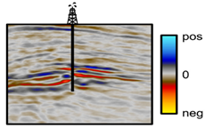
Since the attribute is showing a relative impedance contrast, it can be useful for identifying sequence boundaries, discontinues, and can potentially indicate porosity or fluid content.[32,34]
SweetnessComputed by dividing the envelope by the square root of instantaneous frequency. Geosciences 12 00132 i005
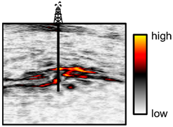
First discovered by Radovich and Oliveros [35], sweetness is a relative value helpful for determining relative net-to-gross ratios and to identify “sweet spots” in hydrocarbon exploration.[35,36,37]
Publisher’s Note: MDPI stays neutral with regard to jurisdictional claims in published maps and institutional affiliations.

