Improvement of GOCE-Based Global Geopotential Models for Gravimetric Geoid Modeling in Turkey

Abstract

This study investigates the contribution of global geopotential models which are calculated with GOCE satellite mission data to the improvement of gravimetric geoid models in Turkey. In this context, direct (DIR), time-wise (TIM), space-wise (SPW), and GOCO satellite-only model series were considered. The research was carried out in two parts. The first part includes the validation of models in each series at 100 homogeneously distributed GNSS/leveling stations over the country utilizing spectrally enhanced geoid heights to determine the best performing model and its optimal expansion degree. According to obtained statistics, the TIM-R6 model was selected as the best model with an optimal expansion degree of 204. In the second part, the TIM-R6 model up to 204 degree/order was linearly blended with EGM2008 to obtain an improved version up to 360 degree/order of expansion. To clarify the contribution of the linearly blended model to the improvement of the regional geoid model, the gravimetric geoid models were computed adopting TIM-R6 up to 204 degree/order and its improved version up to 360 degree/order as reference models. To further emphasize the contribution of the GOCE mission’s data, the gravimetric geoid computations were repeated relying on EGM2008 up to 204 and 360 degrees of expansions, since EGM2008 does not contain GOCE data. In addition, we computed gravimetric geoids based on another combined model that includes GOCE mission data, the EIGEN-6C4 model. The calculated regional geoids were compared to each other and validated using GNSS/leveling data set. The obtained results revealed a ∼23% improvement in regional geoid model accuracy when the blended GOCE-based geopotential model was used as a reference. In addition, the results of this study presented the significance of GOCE contribution to mapping the gravity field in Turkey. The best accuracy obtained from this study was 7.7 cm for the Turkey geoid.

1. Introduction

The modeling of gravity fields using satellites with low Earth orbit has opened a new era in the field of physical geodesy. From the development of the first global gravity field models in the early 1960s to today’s state-of-art global models that can represent the gravity field and its temporal change with unprecedented accuracy, geosciences benefit more and more from the information we can obtain about the Earth’s gravity field and its interior mass significantly [1]. Earth’s gravity field can be modeled with high accuracy using data from geodetic satellite missions that aim to contribute to gravity field studies, namely CHallenging Minisatellite Payload (CHAMP), Gravity Recovery and Climate Experiment (GRACE), and Gravity field and steady-state Ocean Circulation Explorer (GOCE).

The contribution of global geopotential models (GGM) from state-of-art gravity field satellite missions and methodological improvements for gravimetric geoid modeling made it possible the computation of higher accuracy geoid models that can replace the existing vertical datum. Geoid-based vertical datum facilitates obtaining orthometric heights from ellipsoidal heights precisely using Global Navigation Satellite System (GNSS) technologies, hence removing the need for traditional geometric leveling to acquire physical heights. Height systems based on the vertical control network and leveling measurements are gradually replaced with geoid based height systems in countries where a precise regional geoid model is available. In this context, acquiring the optimum data set for the determination of a precise geoid model is of great importance.

The performance of a GGM over an area affects the quality of the gravity field modeling and its parameters. Gravimetric geoid modeling methodologies exploit the GGMs in terms of modeling the long wavelength gravity signals to overcome the absence of these signals in the local gravity data sets. Thus, the increase in the quality of signal content of these models can contribute to the accuracy of regional geoid models, as well. There are studies in the geodetic literature that showed the improvement of the GOCE mission to the regional gravity field modeling [2,3,4,5,6]. Moreover, this increase in the performance of GGMs contributed to the precise estimation of zero-level geopotential value of local vertical datums $W_0^{LVD}$ within the efforts of height system unification studies [7,8,9,10].

Besides its contribution to geodetic applications, the GOCE mission helped us to conduct investigations on the Earth’s interior to further comprehend the geological and geodynamic processes beneath the Earth’s surface [11]. With the first direct observation of the gravity gradients measured from space via the satellite gravity gradiometer (SGG) onboard, the GOCE mission allowed the modeling of the discontinuity surface between the Earth’s crust and upper mantle, known as Moho, more accurately than seismic models as depicted by the assessments against point observations on crustal thickness [12,13]. Aside from the regional improvement achieved in lithospheric structure modeling [14], specifically, the Moho depth [15,16,17] and the upper mantle density [18], the homogeneous distribution of observations obtained from GOCE mission through the entire Earth surface, except for the gaps in polar regions, enabled the estimation of crustal thickness in a global extend [19,20]. Furthermore, the mapping of lithospheric structures via GOCE data paved the wave for detecting the tectonic features on a continental and global scale [21,22,23].

The assessment of the GOCE-based GGMs was conducted with both local and global data sets to report the progress made in the releases of GOCE models, and to clarify the achievement made by GOCE satellite mission [24,25,26,27,28]. These studies showed the contribution of GOCE satellite data to the medium wavelengths of the gravity field in different regions. In Turkey, the performance of the third releases of direct (DIR) and time-wise (TIM) models, second releases of space-wise (SPW) and GOCO models, together with GRACE-only ITG2010S model, were presented in Ince et al. [29]. Later, Erol et al. [30] presented the assessment of all releases of DIR, TIM, and SPW model series, GOCO05S and GOGRA04 models against the same GNSS/leveling data set used in Ince et al. [29], over the entire country. Erol et al. [30] expanded the validation with a closer look to the Marmara region (northwest of Turkey) with 81 GNSS/leveling stations. All studies conducted in Turkey clearly showed the improvement in the medium wavelength components in the gravity field, specifically in the western parts of Turkey where there are precise local GNSS/leveling networks. Nonetheless, the country-wide comparisons in these three studies failed to enunciate the contribution of GOCE considering the limited number of stations. The lack of enough in situ observations thorough the country affected the spectral enhancement results by lowering the level of expected improvement with respect to the performance of the EGM2008 model. Moreover, the spectral bands where the GOCE models exceed the threshold standard deviation of EGM2008 are narrow considering the spectral degrees to which GOCE can contribute. Aside from the comparisons with GNSS/leveling data, Simav and Yildiz [31] presented the evaluation of the fifth releases of DIR, TIM, SPW, and GOCO models against the densified network of relative gravity sites and 16 absolute gravity sites located in the southwest part of Turkey, and showed the improvements in the gravity signals between 120 and 190 degrees.

As different from the above listed studies, this article is on analyzing further improvement capability of the best performing GGM using linear blending approach in Turkey, and testing the consequence of the GGM improvement on the accuracy of regional geoid modeling. Regarding this purpose, prior to the gravimetric geoid model computations, all releases of satellite-only models that are developed based on DIR (R1–R6), TIM (R1–R6), SPW (R1–R5), and GOCO (R1–R6) model series were tested using 100 GNSS/leveling benchmarks distributed homogeneously throughout the entire country. In this evaluation, GGMs, which represent only the part of the spectrum constrained by their maximum degree of expansion, were enhanced spectrally to match their signal content with the observation data which contains the full spectrum of the gravity signal. In this spectral enhancement method, the spectrum beyond the expansion degree/order (d/o) of the model was completed by an ultra-high resolution model EGM2008 [32] and residual terrain effect (RTE) computed from ERTM2160 model [33]. The GGM that showed the best agreement with the in situ data at the optimal degree of expansion (TIM-R6 up to 204 d/o) was determined as a result of this validation. Thereafter, the selected model was improved by completing the coefficients over its optimal degree using the coefficients of EGM2008 up to 360 d/o. To ensure a smooth transition between the coefficients of the two models, the linear blending technique [34] was applied to two coefficient sets near the optimum degree of the GOCE model. The selected GGM (up to its optimal degree) and its improved version (up to 360 d/o) have been employed in the gravimetric geoid modeling based on the least squares modification of Stokes’ integral with additive corrections technique (LSMSA) [35]. The computations of gravimetric geoid models were repeated once more using solely EGM2008 and EIGEN-6C4 [36] up to the optimal d/o of the GOCE model (204 d/o) and the suggested optimal expansion degree (up to 360 d/o) for the gravimetric geoid modeling in Turkey by Isik et al. [37]. Since EGM2008 does not include GOCE mission data, a comparison between the gravimetric geoid models computed with the GOCE-based model and EGM2008 shows the possible contribution of this mission to high-resolution geoid modeling. The calculated six geoid models in the numerical experiment were validated at the GNSS/leveling benchmarks to clarify the differences between the solutions. The findings of this study showed that the improvement in GGM accuracy lead to a significant impact on the accuracy of gravimetric geoid modeling.

This paper consists of four sections. This section introduces the background and objective of the study. In Section 2.1, the tested GGMs are given together with the data used for the spectral enhancement method. The section follows with an explanation of the terrestrial gravity data and briefly describes the pre-processing of the gravity anomaly grid for gravimetric geoid modeling. Section 2.2 includes the theoretical background on the accuracy assessment procedure of GGMs, as well as the formulation for gravimetric geoid modeling. The results of the GOCE-based GGM evaluations and the contribution of the mixed GGM to the performance of the experimental gravimetric geoid models were presented in Section 3. The discussion on the use of the geoid model in geodetic and geodynamic applications is given in the same section. The findings of this paper are summarized in Section 4.

2. Materials and Methods

2.1. Study Area and Data Set

The study was carried out in Turkey between latitudes ${36}^{\circ }\le \phi \le {42}^{\circ }$ and longitudes ${26}^{\circ }\le \lambda \le {45}^{\circ }$. In this section, we started by introducing the GOCE-based GGM that was used in the assessment and continued with the residual terrain model (RTM) which was used to enhance these models spectrally. Following that, we presented the gravity data set used for the gravimetric geoid modeling and briefly explained its pre-processing steps. Finally, we described the GNSS/leveling data set that was used to evaluate both GGMs and calculated experimental gravimetric geoid models in this study.

2.1.1. Global Geopotential Models

From 17 March 2009 to 11 November 2013, GOCE continued to revolve in its orbit at approximately 250 km altitude, providing unprecedented detail of the stationary gravity field of Earth. The mission flew at its unusually low orbital height for four years, measuring the second derivative of the gravity potential using a satellite gravity gradiometer (SGG) while its orbit was being tracked via high-to-low satellite-to-satellite tracking (hl-SST). The aim of the mission was to determine gravity anomalies with an accuracy of 1 mGal and the geoid with 1–2 cm at 100 km spatial resolution, corresponding to 200 degree/order harmonic expansion [38].

So far, various gravity field solutions have been computed using GOCE satellite data. Specifically, the solutions of the High-Level Processing Facility (HPF) of GOCE are of great importance for processing GOCE data to produce gravity field solutions using three different approaches, namely direct, time-wise, and space-wise. The first releases of these model series include only 2 months of GOCE data. The second, third, and fourth releases were computed using 8 months, 18 months, and 33 months of GOCE observations, respectively. The full mission data (48 months) is used for the fifth and sixth releases.

The DIR approach is based on the computation of spherical harmonic coefficients using an iterative solution of SST and SGG normal equations together that are formed for each batch of 24 h (daily) arcs. The normal equations of daily arcs are then stacked, and solved by using Cholesky decomposition. This approach requires a priori weights from a reference gravity field model [26]. In the first release of DIR models (DIR-R1), the a priori gravity field information is taken from the EIGEN5C model up to degree/order 360. In the second release (DIR-R2), the reference model is replaced by the ITG-Grace2010s model up to 150 degree/order. The releases after DIR-R2 used one release before as the a priori model (e.g., the DIR-R2 is a priori model for the computation of the DIR-R3 model). In the TIM computation schema, SST and SGG data measured along the satellite orbit are treated as a time series. The gravity field models computed using the TIM approach are pure GOCE solutions, containing no other measurements from CHAMP, GRACE, or a priori model. This is beneficial in terms of seeing how good of a solution can be achieved based on solely GOCE observation. The SPW approach, on the other hand, is based on the solution of least squares collocation that uses the spatial correlation of the gravity field with the distance to form a signal covariance. The method deals with the SST and SGG measurements in the spatial domain, as opposed to the time/frequency domain, by gridding them via least squares collocation, as well. As a prior model, the first release (SPW-R1) uses EGM2008 in very low degrees and Quick-look gravity field model. There is no a priori model used for the computation of SPW models from the second release (SPW-R2) to the last (SPW-R5), aside from the use of the EIGEN model series for the signal covariance modeling and the FES2004 tide model for ocean tide modeling. This makes these SPW releases GOCE-only solutions. More details about the philosophy behind these methodologies and the computation schema of these approaches are extensively discussed in [26]. To exploit the GOCE satellite mission at best, the combination of the observations from other dedicated missions provides a better representation of long-wavelength signals. In this context, the initiative called Gravity Observation Combination (GOCO) provides gravity field solutions for satellite-only models by combining the data from CHAMP, GRACE, GOCE, and SLR [39].

In the first part of the numerical tests, all releases of DIR [40,41,42], TIM [26,43,44,45], SPW [46,47,48,49] and GOCO [39,50,51,52,53] satellite-only models were included in the determination of the most suitable GOCE-based GGM for Turkey. The satellite data content and maximum degree of expansion of these models are given in

Table 1. Tested global geopotential models and their data content.

Model	Max Degree	Data
DIR R1	240	GOCE (2 m)
DIR R2	240	GOCE (8 m)
DIR R3	240	GOCE (18 m), GRACE (6.5 y), SLR (6.5 y)
DIR R4	260	GOCE (33 m), GRACE (9 y), SLR (>10 y)
DIR R5	300	GOCE (48 m), GRACE (>10 y), SLR (>10 y)
DIR R6	300	GOCE (48 m), GRACE (>10 y), SLR (>10 y)
TIM R1	224	GOCE (2 m)
TIM R2	250	GOCE (8 m)
TIM R3	250	GOCE (18 m)
TIM R4	250	GOCE (33 m)
TIM R5	250	GOCE (48 m)
TIM R6	300	GOCE (48 m)
SPW R1	210	GOCE (2 m)
SPW R2	240	GOCE (8 m)
SPW R4	280	GOCE (33 m)
SPW R5	330	GOCE (48 m)
GOCO0S R1	224	GOCE (2 m), GRACE (7.5 y)
GOCO0S R2	250	GOCE (8 m), GRACE (7.5 y), SLR (5 y)
GOCO0S R3	250	GOCE (18 m), GRACE (7.5 y), SLR (5 y)
GOCO0S R5	280	GOCE (48 m), GRACE (10.5 y), CHAMP (6 y), SLR (>10 y)
GOCO0S R6	300	GOCE (48 m), GRACE (15.5 y), CHAMP (6 y), SLR (>10 y)

m: month, y: year.

.

2.1.2. Residual Terrain Model

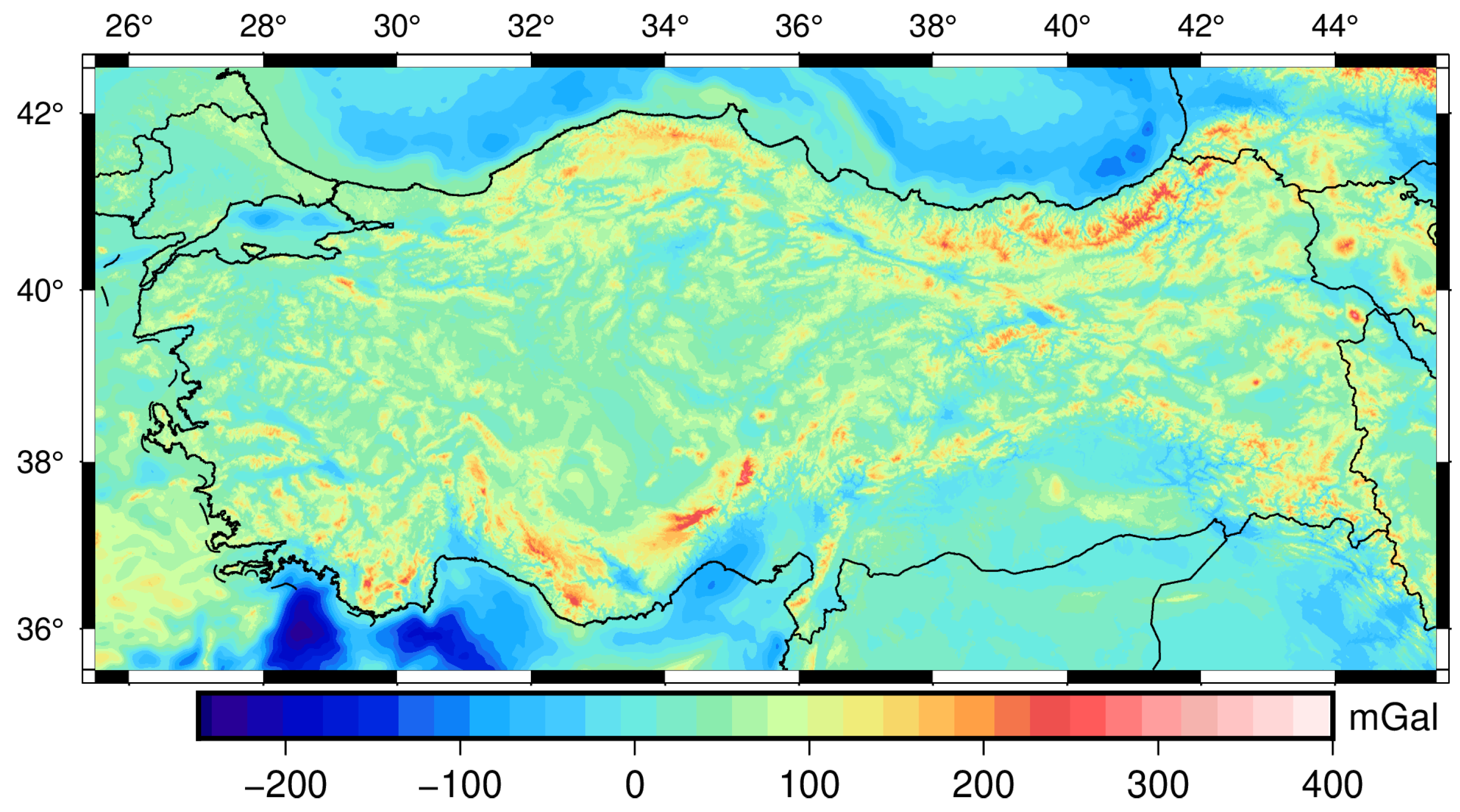
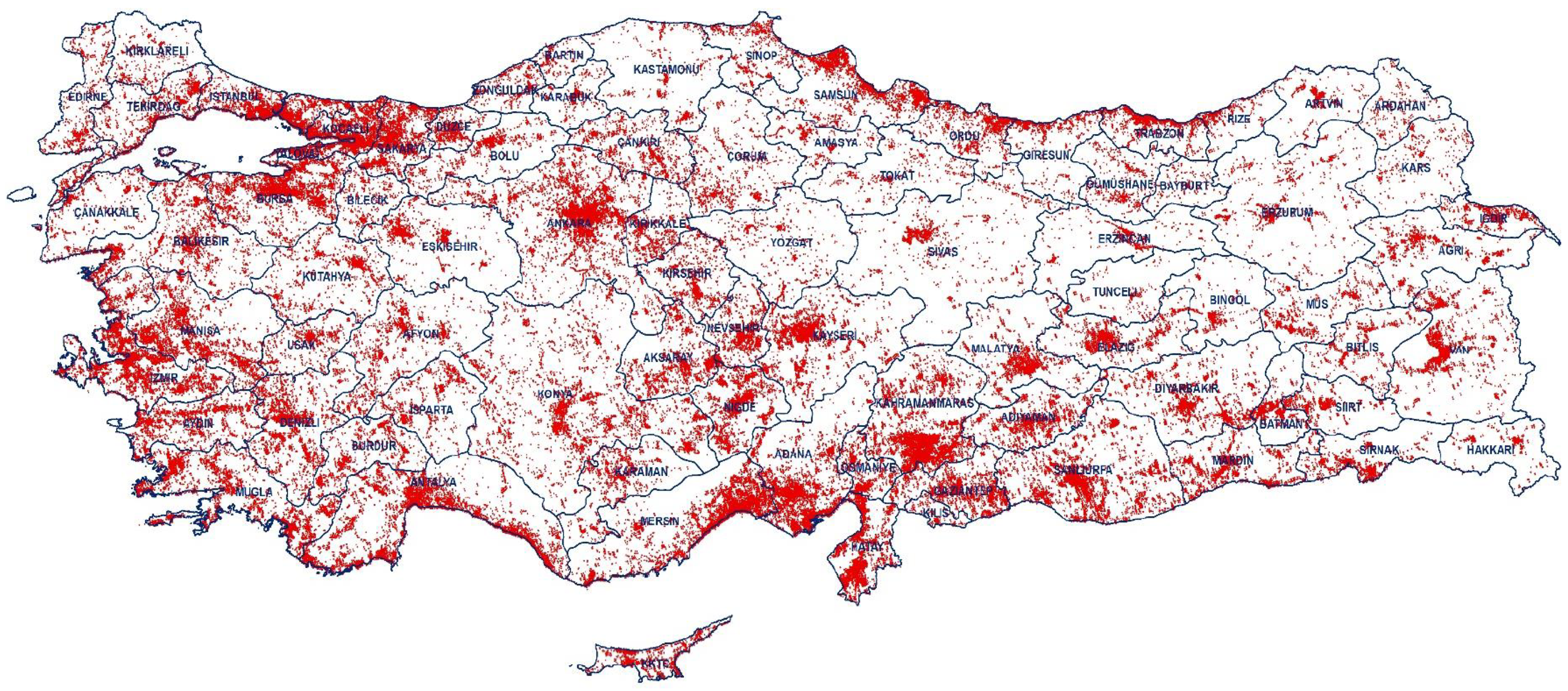
RTMs are used in many geodetic and geophysical applications that require high frequency, accordingly short wavelength, gravity signal information. These models are mainly used in the completion of gravity signals beyond the expansion degree of a GGM to augment its spectral content. Another frequent use of RTM is seen in studies that deal with smoothing the gravity observations, either terrestrial or airborne, before interpolating them to create gridded data (i.e remove–grid–restore) or to reduce the computational error of upward/downward continuation. Additionally, it is one of the main steps of a well-known geoid modeling technique, remove-compute-restore.

In this study, our intent to use RTM is to enhance the GGMs spectrally beyond 2159 degree/order. We used ERTM2160 computed from 7.5″ resolution SRTM topography that corresponds to the signal content between ∼10 km to ∼250 m [33]. The model includes the high-frequency gravity signals for four gravity field parameters, namely quasigeoid/geoid, gravity disturbance, and north–south and east–west components of vertical deflection according to Helmert’s definition. Since we are only interested to validate the GGMs against GNSS/leveling data, we used only RTE on geoid. Figure 1 shows the magnitude of RTE from the ERTM2160 model on geoid in Turkey, along with its statistics.

2.1.3. Gravity Data

The gravity measurements have been collected by the General Directorate of Mineral Research and Exploration (GDMRE) [54]. The data set originally contains 64,469 gravity measurements with 3.5 km spacing throughout the country. However, it must be noted that we only have the gridded version of the gravity data as a complete Bouguer anomaly. The scattered gravity data are not open for scientific use. This archival data set originally was tied to the Potsdam datum for gravity. We added −14 mGal to the grid values to convert them to International Gravity Standardization Net 1971 (IGSN71) datum. GDMRE processed the reduction of the gravity data by taking the mass density of the Bouguer plate as 2.67 g/cm³ while assuming a mass density of topography as 2.40 g/cm³ in the terrain correction. The effect of terrain on the gravity measurements was computed within 6.65 km radius for each gravity point, as the original data includes the terrain correction up to J-zone in Hammer chart [55]. To comply with these pre-processing parameters applied by GDMRE, we have employed the same parameters in the conversion of complete Bouguer anomalies to free-air anomalies. Finally, the normal gravity values that were originally calculated using the GRS67 reference ellipsoid were converted to GRS80 ellipsoid. The complete (or refined) Bouguer anomalies were converted to free-air gravity anomalies to be used as an input for gravimetric geoid modeling. Please refer to Isik et al. [37] for details of the processing of the GDMRE complete Bouguer anomaly grid for the computation of free-air anomalies shown in Figure 2.

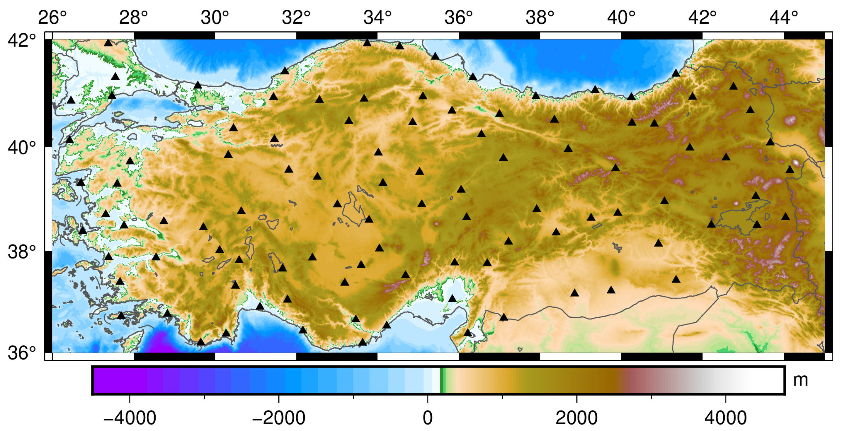
2.1.4. Validation Data Set

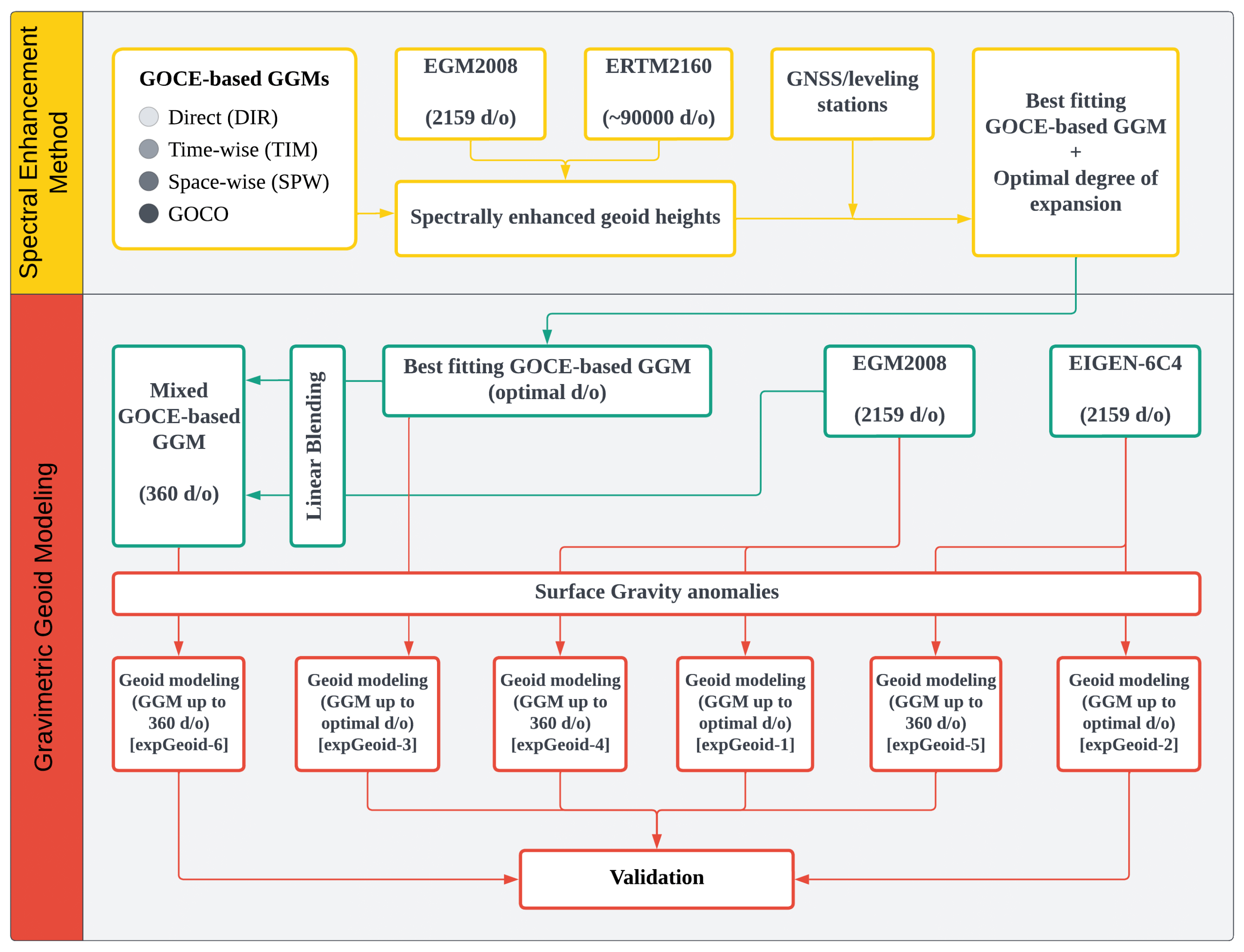
In this study, we used 100 GNSS/leveling stations that are part of common benchmarks of the Turkish National Fundamental GPS Network (TUTGA) and the Turkish National Vertical Control Network 1999 (TUDKA99). The GNSS measurements in these benchmarks are at least 8 h long, and the coordinates are in International Terrestrial Reference Frame 1996 (ITRF96) datum. The physical heights, on the other hand, are Helmert orthometric heights measured according to the regulation for the 1st order leveling network requirements with forward and backward leveling. The accuracy of these GNSS/leveling data set is reported as ∼1–3 cm [56]. The distribution of the GNSS/leveling stations above the topography of Turkey from SRTM 3” resolution digital elevation model [57] is given in Figure 3.

The geoid heights at GNSS/leveling stations are computed as,

$$N_{GNSS/leveling}=h-H$$

(1)

where h is the ellipsoidal height from GNSS measurements and H is the Helmert orthometric height from geometric leveling. In the validation of geoid models, either gravimetric geoid or synthesized from GGMs, the geoid heights refer to a tide-free permanent tide system. By convention, the ellipsoidal heights are computed in a tide-free system. In order to make GNSS/leveling derived geoid heights comparable with the others, the permanent tide system of Helmert orthometric heights at GNSS/leveling stations were converted from mean-tide to tide-free system as,

$$H^{\mathrm{tide}\mathrm{free}}=H^{\mathrm{mean}\mathrm{tide}}-0.68\left(0.099-0.296{sin}^2\phi \right)$$

(2)

where $H^{\mathrm{tide}\mathrm{free}}$ and $H^{\mathrm{mean}\mathrm{tide}}$ are the tide-free (or non-tidal) and mean-tide orthometric heights, and $\phi$ is the latitude of the GNSS/leveling station [58].

2.2. Methodology

In this section, we provide the details of the methodology applied to clarify the importance of the selection of GGM and its signal content to be constrained by the expansion degree that fits best with the in situ measurement, and its impact on the accuracy of the gravimetric geoid model. The source of the long-wavelength signal content computed from the GGM plays an important role in achieving the best solution. In this regard, the computation strategy adopted in this study begins with the determination of the best performing GOCE-based GGM and its optimal degree of expansion, as prior to the gravimetric geoid modeling. The first part explains how the GOCE-based models were validated in terms of geoid heights by using the spectral enhancement method to make the models spectrally comparable with the GNSS/leveling data set. This section is followed by the gravimetric geoid modeling approach based on the stochastic modification of Stokes’ integral that minimized the expected global mean square error of the geoid model considering the errors introduced by the GGM and terrestrial gravity data. The steps of the methodology can be followed via the flowchart of this study given in Figure 4.

2.2.1. Spectral Enhancement Method

The quasi-geoid heights $\left(\zeta \right)$ can be calculated using coefficients of disturbing potential via spherical harmonic expansions as,

$${\zeta }_{GGM}=\frac{GM}{r\gamma }\sum _{n=2}^{n_{max}}{\left(\frac{a}{r}\right)}^n\sum _{m=0}^n\left(\Delta {\overline{C}}_{nm}cosm\lambda +{\overline{S}}_{nm}sinm\lambda \right){\overline{P}}_{nm}\left(\cos \theta \right)$$

(3)

where G is the gravitational constant, M is the mass of the Earth, a is the semi-major radius and $\gamma$ is the normal gravity of the reference ellipsoid, $\Delta {\overline{C}}_{nm}$ and ${\overline{S}}_{nm}$ are the spherical harmonic coefficients of disturbing potential at degree n and order m, ${\overline{P}}_{nm}$ is the fully normalized Legendre functions, and finally $\theta$, $\lambda$ and r are the coordinates of the computation point which are co-latitude, longitude, and local radius, respectively. Since the coefficients of the GGM represent the gravity potential W, the normal potential must be removed from the gravity potential to form disturbing potential T where $T=W-U$. This is handled as,

$$\Delta {\overline{C}}_{nm}={\overline{C}}_{nm}^W-{\overline{C}}_{nm}^U$$

(4)

where ${\overline{C}}_{nm}^W$ and ${\overline{C}}_{nm}^U$ are the spherical harmonic coefficients of gravity potential W and normal potential U, respectively. Because of rotational and equatorial symmetry of normal potential, ${\overline{C}}_{nm}^U$ contains only even zonal harmonics, i.e., only the terms where the order m is zero ($C_{2,0}^U,C_{4,0}^U,\cdots$) [1].

In case the physical heights of the GNSS/leveling stations are orthometric heights, as opposed to normal heights, the quasi-geoid heights, calculated from the GGM using Equation (3), must be converted to geoid heights using geoid-to-quasigeoid separation term. This term can be approximated using the simple Bouguer anomaly $\Delta g_{BA}$, the mean normal gravity $\overline{\gamma }$, and the orthometric height H at the computation point as Equations (8)–(113) of [59],

$$N-\zeta =\frac{\Delta g_{BA}}{\overline{\gamma }}H$$

(5)

While evaluating the performance of GGMs using GNSS/leveling data in an absolute sense, the geoid heights from GGMs are compared with the geoid heights derived from the GNSS/leveling observations. These observations, in nature, contain the full spectrum of the gravity signal, as opposed to the ones computed from GGMs. The geoid heights computed from the spherical harmonic expansions, as formulated in Equation (3), contain gravity signals up to a degree to which the GGM is expanded. This shortage in the contained gravity signal is caused by the limitation of the GGM constrained by its maximum degree of expansion. The absence of gravity signals above the maximum degree in spherical harmonic expansion causes an error called omission error [25].

In order to make the GGM and observation data spectrally comparable and remove the effect of omission error as much as possible, the model can be enhanced by using another model with a higher expansion degree (possibly an ultra-high resolution model) and RTM to complete the short-scale gravity signals. The evaluation of geoid heights calculated from GGMs based on the spectral enhancement method is as follows [25],

$$N_{res}=N_{GNSS/leveling}-\left(N_0+{\left.N^{GOCE}\right|}_2^n+{\left.N^{EGM2008}\right|}_{n+1}^{2159}+{\left.N^{RTE}\right|}_{2160}^{\infty }\right)$$

(6)

where $N_{res}$ is the residual geoid heights, $N_{GNSS/leveling}$ is the geoid heights derived from ellipsoidal height and orthometric heights at the control station, $N_0$ is the zero-degree term geoid height, ${\left.N^{GOCE}\right|}_2^n$ is the geoid height calculated from the GOCE model in evaluation using harmonic degrees from 2 to n, ${\left.N^{EGM2008}\right|}_{n+1}^{2159}$ is the geoid height calculated from a high-resolution model such as EGM2008, and ${\left.N^{RTE}\right|}_{2160}^{\infty }$ is the geoid height that represents the short wavelength signals beyond the maximum degree of high-resolution model $n_{max}=2160$.

In Equation (6), the spherical harmonic expansion starts from degree 2, omitting the terms formed by zero-degree and first-degree. With the choice of a coordinate system that coincides with the geo-center of the Earth, the first-degree terms can be easily omitted. The zero-degree term is handled externally to account for different mass estimates of the GGM that represents the gravity potential W and the reference ellipsoid that represents the normal potential U in the computation of disturbing potential. The zero-degree term geoid height, given in Equation (6), is computed as follow [60]:

$$N_0=\frac{\left(G{M}_{GGM}-G{M}_{\mathrm{ELL}}\right)}{r_{P_0}{\gamma }_{Q_0}}-\frac{W_0-U_0}{{\gamma }_{Q_0}}$$

(7)

where $r_{P_0}$ is the geocentric radial distance for the computation point, and ${\gamma }_{Q_0}$ is the normal gravity on the reference ellipsoid. The first term on the right-hand side of Equation (7) represents the component of zero-degree term caused by the mass difference $\delta M$ between the GGM and the reference ellipsoid ($\delta M=M_{GGM}-M_{ELL}$). The second term, on the other hand, is the result of the difference between the potential of the Earth $W_0$, represented by the conventional value adopted by the International Association of Geodesy [61], and the normal potential of the reference ellipsoid.

The RTE represents the forward modeling of gravity to achieve the short-scale gravity signals occurred by the existence of topographic masses. In Equation (6), the RTE does not play a role in the determination of the optimum expansion degree of the GGM, since the omission errors for the spectrally enhanced models beyond 2159 d/o are the same. However, the RTE term reduces the magnitude of the residual geoid heights, hence the standard deviation of the residuals becomes smaller. The formulation of RTE on geoid ($N_{RTE}$) can be found in [62] and the details of the computation strategy of RTM can be found in Hirt et al. [33].

2.2.2. Gravimetric Geoid Modeling

The Stokes’ integral enables the computation of geoid using gravity observations, as the solution of the geodetic boundary value problem. In this computation, there are certain assumptions and requirements to be able to model the geoid surface. One of which is the necessity of gravity data in the entire Earth since the integration is conducted globally for each computation point. This is not possible in practice for many reasons. The implementation of Stokes’ integral in a small region causes a truncation error. Furthermore, the absence of gravity observations outside the computation region, and the limitations of the spatial resolution of the terrestrial gravity data set to result in long-wavelength errors in the gravity field. These problems create the necessity to modify the Stokes’ kernel. With the first study conducted by Molodenskii et al. [63], and many more that attempt to modify the Stokes’ kernel in a deterministic or stochastic approach, the foundations of today’s precise techniques of gravimetric geoid modeling are built. See Ellmann [64] for details of the prominent modification methods of Stokes’ integral with a case study for geoid modeling in Baltic countries. Sjöberg [35] proposes a new technique to determine gravimetric geoid by using spectrally modified Stokes’ kernel that deals with the truncation error, as well as the spectral weighting of satellite and terrestrial gravity data determined by their error information. In this method, the least squares modification of Stokes’ formula is implemented to minimize the expected global mean square error by optimally combining the GGM and terrestrial gravity data. The main formula of this methodology is given as,

$$\hat{N}=\tilde{N}+\delta N_{COMB}^{TOPO}+\delta N_{COMB}^{DWC}+\delta N_{COMB}^{ATM}+\delta N_{COMB}^{ELL}$$

(8)

where the first term on the right-hand side represents the approximate geoid heights, and the rest of the terms represent the so-called additive corrections to calculate the detailed geoid model.

The approximate geoid height $\tilde{N}$,

$$\tilde{N}=\frac{R}{4\pi \gamma }\underset{{\sigma }_0}{\int \int }{S}^L\left(\psi \right)\Delta gd\sigma +\frac{R}{2\gamma }\sum _{n=2}^M(s_n+Q_n^L)\Delta g_n^{GGM}$$

(9)

where the first term in the right-hand side of Equation (9) is the near-zone component calculated using the surface gravity anomalies $\Delta g$ within the integration cap ${\sigma }_0$ via modified Stokes’ kernel ($S^L\left(\psi \right)$). The second term in this equation is the far-zone component of the geoid signal calculated from the GGM via Laplace harmonics of gravity anomalies $\Delta g_n^{GGM}$ up to expansion degree M Equations (9)–(18) of [59], the modification parameters $s_n$, and the truncation coefficients $Q_n^L$. For more details, please refer to Sjöberg [35].

Out of the corrections given in Equation (8), $\delta N_{COMB}^{TOPO}$ is the combined topographic correction to deal with both direct and indirect topographic effects of the mass above the geoid surface [65]. $\delta N_{COMB}^{DWC}$ is the combined downward continuation correction to take into account the use of surface gravity anomalies in modified Stokes’ integral, as opposed to gravity anomalies on geoid surface. This gives an advantage of not dealing with the downward continuation of gravity anomalies to the geoid surface, which is an ill-posed problem, but rather computing its effect directly on the geoid [66]. $\delta N_{COMB}^{ATM}$ is the combined atmospheric correction for the atmospheric mass [67], and finally, $\delta N_{COMB}^{ELL}$ is the combined ellipsoidal correction for the spherical approximation of Stokes’ integral in the computation of geoid [68].

3. Results and Discussions

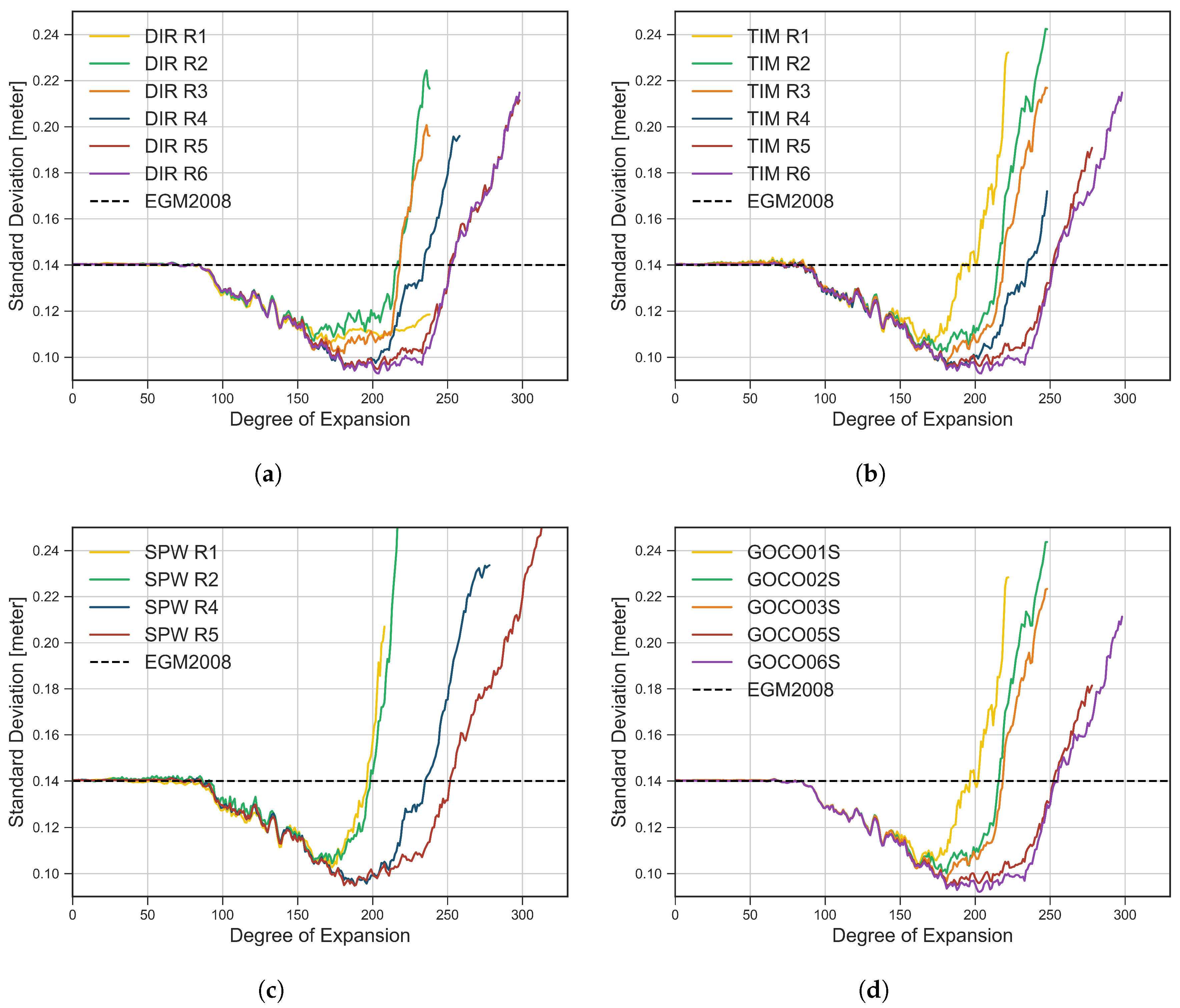
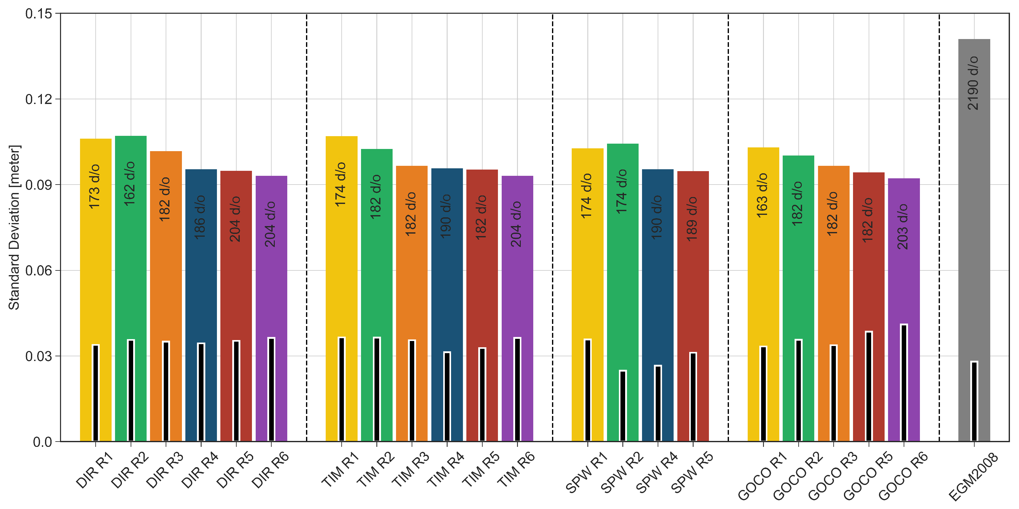
3.1. Assessment of Global Geopotential Models

We applied spectral enhancement to all GGMs given in Section 2.1.1 to calculate geoid heights for each degree of expansion from $n=2$ to $n=n_{max}$ with one degree/order increment. The zero-degree term geoid height $N_0$ was added to account for the systematic difference between the mean earth ellipsoid of the GGM and the GRS80 ellipsoid on which we adopted to reference the computations. All computations of geoid heights were carried out in a tide-free permanent tide system.

The standard deviations of residual geoid heights for each spectrally enhanced GOCE model are presented in Figure 5. The horizontal axis of the figures represents the degree to which the tested GOCE model is expanded, while the vertical axis shows the change in the standard deviation of the residuals as the expansion degree of the GOCE model increases. The rest of the gravity signals beyond the expansion degree of the tested model was filled from EGM2008 up to 2159 degree and RTM from 2159 to 90,000. The black dashed line represents the standard deviation of the residual geoid heights achieved by expanding EGM2008 up to 2159 degree/order and enhancing with RTE, which corresponds to 14.1 cm accuracy.

In all four figures that represent the performance of different model series, the contribution of the GOCE mission between ∼100 degree/order and ∼250 degree/order is visible. The geoid heights from all releases of the model series showed better agreement with the geoid heights at GNSS/leveling benchmarks compared to the EGM2008 model in these spectral bands. The results clearly show the improvement in the accuracy of models from the first releases to the last for all model groups. The increase in the amount of GOCE satellite data led to a decrease in the standard deviations of the residual geoid heights at the GNSS/leveling stations, as well as the spectral window of bands that showed improvement over EGM2008 is wider in the latest releases.

For DIR, TIM, and GOCO model series, the fifth and sixth releases showed similar improvements. Between ∼200 and ∼245 degree/order of the spectrum, the sixth releases of TIM and GOCO exceeded the performance of the fifth releases. Their performances can be considered as equal outside of these spectral bands. For the SPW model series, the fourth and the fifth releases gave almost the same result up to the degree/order ∼210. The fifth (and final) release became prominent after this degree, and SPW-R5 showed 5 cm better agreement at the maximum degree of SPW-R4 ($n_{max}=280$).

From the first to the last releases, we see over 10% improvements in standard deviations of the model series. With 9.3 cm accuracy around ∼204 degree/order expansion, DIR-R6, TIM-R6, and GOCO06S models were found to be the best performing models in Turkey. The overall view of the best performing degree of GGMs is presented with their standard deviations and means in Figure 6, and the statistics of the residual geoid heights of best performing GOCE model in each model serie is given in

Table 2. Statistics of the residual geoid heights of best performing spectrally enhanced GOCE models at optimum expansion degree [unit: cm].

GGM	Degree	Min	Max	Mean	SD
DIR-R6	204 *	−22.2	28.7	3.7	9.3
TIM-R6	204 *	−22.4	28.4	3.7	9.3
SPW-R5	189 *	−18.2	25.7	3.1	9.5
GOCO06S	203 *	−22.0	30.8	4.2	9.3
EGM2008	2190	−27.7	42.0	2.9	14.1

* The optimal degree of the model expanded to 2190 d/o.

.

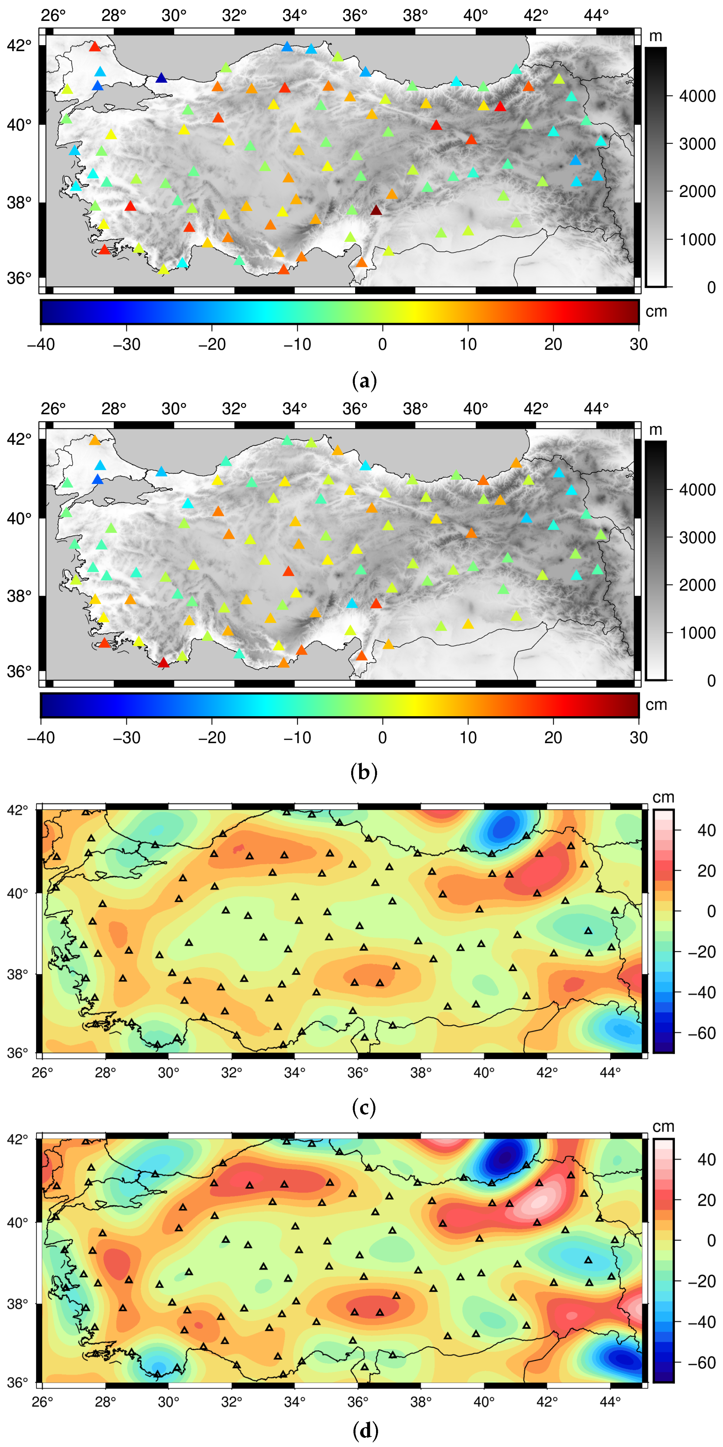
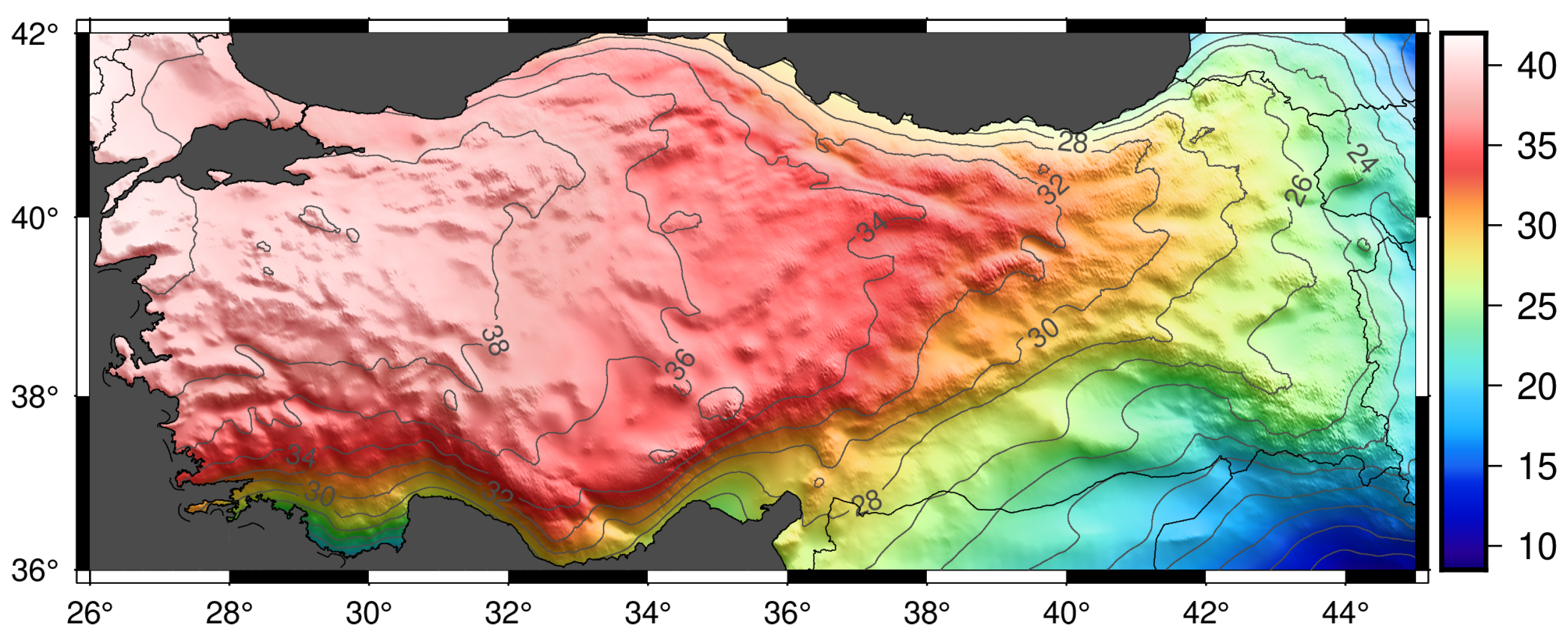
3.2. Determination and Validation of Gravimetric Geoid Models

We implemented the least squares modification of Stokes’ integral approach to model the gravimetric geoid in Turkey based on EGM2008, EIGEN-6C4, and TIM-R6 GGMs. As a combined model with ultra-high resolution, EGM2008 was used in many regional geoid models, not only for former official Turkey Geoid models but also for other countries as well. Additionally, it was computed before the GOCE era which makes this model valuable for showing the contribution of the GOCE mission. As the best GGM with the smallest standard deviation against the GNSS/leveling data set, TIM-R6 is the most suitable model to clearly show the improvements in the gravimetric geoid model, considering it is a pure GOCE model. EIGEN-6C4 is also an ultra-high resolution combined model just like EGM2008. The most significant aspects of the EIGEN-6C4 that diverge from the EGM2008 model are the contribution of GOCE satellite data and improved surface gravity data sets. Thus, the comparison of the gravimetric geoid model computed with GOCE-based combined GGM provides another perspective on the expected improvement brought by the GOCE satellite mission.

The experimental geoid models were computed in a tide-free system and the zero-degree term was calculated w.r.t. GRS80 reference ellipsoid. In the computation of the least squares modification parameters $s_n$ and $Q_n^L$, the integration radius around the computation points was taken as ${\psi }_0=0.{25}^{\circ }$ in the Stokes’ integral. The error degree variance of gravity anomalies was constructed using a band-limited white noise model where the standard deviation is taken as ${\sigma }_{\Delta g}=5$ mGal. The values of modification parameters for the gravimetric geoid modeling were adopted from the experimentation conducted by Isik et al. [37] to empirically determine the optimum values of modification parameters (${\psi }_0=0.{25}^{\circ }$, $M=360$, and ${\sigma }_{\Delta g}=5$ mGal) for LSMSA technique in Turkey.

As an expansion (M) and modification degree (L) where $M=L$, we first implemented a modification degree $M=204$ for gravimetric geoid models computed with EGM2008 (expGeoid-1), EIGEN-6C4 (expGeoid-2) and TIM-R6 (expGeoid-3), since this expansion degree was found as the optimum degree for the last releases of GOCE models. Later, the GGMs were used up to 360 degree to enhance the geoid accuracy. Though this degree can be implemented for the EGM2008 (expGeoid-4) and EIGEN-6C4 (expGeoid-5) models, it is not possible for the TIM-R6 model because of its limited maximum degree ($n_{max}^{TIM-R6}=300$). To improve the gravimetric geoid modeling results, we combined the coefficients of EGM2008 with the TIM-R6 model to make a mixed model up to 360 degree/order, as this degree was found as the optimum for regional geoid in Turkey [37]. The maximum combination degree of the EGM2008 and GOCE model was determined based on the assessment results of the TIM-R6 model using the spectral enhancement method. The optimum combination degree was found to be 204 for the GOCE model where the rest of the gravity spectrum was filled with EGM2008 and RTM. From degree $n=2$ to $n=204$, TIM-R6 model coefficients were used. The gravity spectrum between degrees 215–360 is filled with EGM2008 coefficients. The coefficients in the spectral band between 205–214, were determined by taking the mean of the coefficients of two models based on weights determined by their error information in order to blend the coefficients of two models linearly, as in the earlier studies that combined EGM2008 with GOCE model to improve the long-wavelength signal [34,69,70],

$$T_{mn}=\left[\frac{T_{mn}^{EGM2008}}{{\left({\sigma }_{T_{mn}}^2\right)}^{EGM2008}}+\frac{T_{mn}^{TIM}}{{\left({\sigma }_{T_{mn}}^2\right)}^{TIM}}\right]{\left[\frac{1}{{\left({\sigma }_{T_{mn}}^2\right)}^{EGM2008}}+\frac{1}{{\left({\sigma }_{T_{mn}}^2\right)}^{TIM}}\right]}^{-1}$$

(10)

where $T_{mn}$ represents the new coefficients $C_{mn}$ and $S_{mn}$ of disturbing potential T, $T_{mn}^{EGM2008}$ and $T_{mn}^{TIM}$ represent the corresponding coefficients of EGM2008 and TIM-R6 models, and ${\left({\sigma }_{T_{mn}}^2\right)}^{EGM2008}$ and ${\left({\sigma }_{T_{mn}}^2\right)}^{TIM}$ are the degree variances of $T_{mn}^{EGM2008}$ and $T_{mn}^{TIM}$, respectively. For more details about the methodology, please refer to Gilardoni et al. [34].

The statistics of residual geoid heights computed from the gravimetric geoid models at GNSS/leveling stations are given in

Table 3. Statistics of gravimetric geoid model accuracy computed using TIM R6, EGM2008, and EIGEN6C4 models. [unit: cm].

Geoid Model	Reference GGM		Min	Max	Mean	SD
expGeoid-1	EGM2008 ($M=204$)	Before fit	−62.7	56.6	−1.2	20.5
		After fit	−50.5	59.7	0.0	19.3
expGeoid-2	EIGEN-6C4 ($M=204$)	Before fit	−60.1	53.7	−0.7	20.0
		After fit	−50.3	46.6	0.0	18.1
expGeoid-3	TIM-R6 ($M=204$)	Before fit	−58.5	53.2	−0.2	20.1
		After fit	−50.0	42.0	0.0	18.4
expGeoid-4	EGM2008 ($M=360$)	Before fit	−37.0	29.7	−0.3	11.5
		After fit	−33.9	35.6	0.0	10.3
expGeoid-5	EIGEN-6C4 ($M=360$)	Before fit	−25.6	20.2	−1.6	9.2
		After fit	−20.5	20.6	0.0	7.9
expGeoid-6	TIM-R6 + EGM2008	Before fit	−24.6	23.5	0.7	8.9
	(mixed model − $M=360$)	After fit	−20.2	17.5	0.0	7.7

, together with the statistics of the residual geoid heights after the geoid models were fitted to local vertical datum at GNSS/leveling stations using seven parameter Helmert similarity transform [71]. The experimental geoid models computed with EGM2008, EIGEN-6C4, and TIM-R6 models up to 204 degree/order expansion, namely expGeoid-1, expGeoid-2, and expGeoid-3, have shown ∼20 cm accuracy against the GNSS/leveling data set. All three models failed to supersede the performance of the EGM2008 GGM up to 2159 degree/order. The gravimetric geoid model computed with EGM2008 up to 360 degree/order (expGeoid-4) has a standard deviation of $11.5$ cm ($10.3$ cm after-fit) where the standard deviation of $9.2$ cm ($7.9$ cm after-fit) was achieved for the gravimetric geoid computed with EIGEN-6C4 (expGeoid-5). The gravimetric geoid model computed with the mixed geopotential model (expGeoid-6) has shown $8.9$ cm ($7.7$ cm after-fit). Using 360 d/o of expansion for the GGM drastically improved the accuracy of the geoid model due to the long-wavelength errors in the gravity anomaly data used in the geoid modeling. The low quality of gravity signals below 360 d/o is compensated by the long-wavelength information from GGM. Similar findings were observed by Isik et al. [37] using a GOCE-based GGM XGM2019. The results showed that the use of a mixed geopotential model as a long-wavelength source has led to an improvement of ∼23% in the accuracy of the gravimetric geoid model. Out of these three gravimetric geoid models computed with 360 degree/order expansion of GGM, the performance of the model computed with the EGM2008 (expGeoid-4) revealed ∼2.5 cm worse agreement against the observation data. The performance of the gravimetric geoid models expGeoid-5 and expGeoid-6 are quite similar to each other due to the inclusion of GOCE data as long-wavelength information. Though the improvement brought by expGeoid-6 is not significantly greater than that of expGeoid-5, the use of the mixed model for the gravimetric geoid modeling (expGeoid-6) demonstrated the best agreement with the GNSS/leveling derived geoid heights.

The distribution of geoid height differences for the gravimetric geoid models computed using the EGM2008 (expGeoid-4) and the TIM-R6/EGM2008 mixed GGM (expGeoid-6) at GNSS/leveling benchmarks was plotted in Figure 7a,b over the topography of Turkey to show the variations brought by the use of GOCE-based GGM. The residual geoid heights for the expGeoid-6 model are significantly smaller compared to expGeoid-4. The contribution of GOCE resulted in a decrease of 18.6 cm in the range of residual geoid heights, from 66.7 cm for expGeoid-4 to 48.1 cm for expGeoid-6. The varying behavior of these two gravimetric geoid models, given as a difference grid in Figure 7c, can be attributed to the large amplitudes of long-wavelength geoid differences between EGM2008 and TIM-R6 model up to 204 degree/order expansion (Figure 7d). Since the expansion degree of both models in Figure 7d is the same, the geoid height differences are not affected by the omission errors of the models. The large discrepancies between the residual geoid heights of expGeoid-4 and expGeoid-6 at GNSS/leveling heights are visible in areas where the long-wavelength differences in Figure 7d are larger, specifically along the northern coastlines. A closer look to the northeast part of Turkey shows an abrupt change in the long-wavelength differences (from $\sim -$70 cm to ∼50 cm) between TIM-R6 and EGM2008 models.

The gravimetric geoid model, expGeoid-6, has shown the best performance compared to the other five experimental geoid models against 100 GNSS/leveling stations. Considering the accuracy of the geoid models reported by the previous studies that used the same terrestrial gravity data set, this model has the lowest standard deviation [30]. Most recently, the accuracy of the LSMSA geoid model computed using XGM2019e GGM up to 360 degree/order was stated as $10.1$ cm by Isik et al. [37], leading to ∼13.9% better performance than expGeoid-4 and ∼13.5% worse performance than expGeoid-6 at the same GNSS/leveling benchmarks. Moreover, expGeoid-6 outperforms the geoid model presented by Isik et al. [37] in terms of the range of residual geoid heights by $5.2$ cm. The models’ performance exceeds the accuracy of the gravimetric geoid model computed via the least squares modification of Hotine’s integral (LSMHA) method, which was reported as $10.4$ cm by Isik et al. [72].

The expGeoid-6, as the gravimetric geoid model with the best standard deviation, is presented in Figure 8 together with its statistics. The accuracy of the geoid model is $7.7$ cm after it is fitted to the local vertical datum via a seven-parameter model at the GNSS/leveling benchmarks.

3.3. Discussion on the Use of Geoid Model

The gravimetric geoid model, from the geodetic point of view, is of great importance for forming an equipotential surface for the determination of the physical heights. Conventionally, this task is untangled by taking the mean sea level surface, which is approximated by the geoid surface, as the reference zero-level and carry the height information via traditional geodetic leveling. As precise as this method is, it is both expensive and requires laborious work to do leveling across the country, not to mention the measurement errors building up quickly as we move further away from the zero-level.

The determination of an accurate gravimetric geoid model that modernizes the regional vertical datum is essential for the improvement of the geo-spatial data infrastructure in a country and for providing reliable physical height information that contributes to the environmental, geophysical, and geodynamic processes in different levels of Earth’s system. Such a geoid model that can replace the traditional mean sea level based vertical datum requires ∼1–2 cm accuracy throughout the country. The required level of accuracy needs certain decisions to be considered in the geoid modeling methodologies, one of which is the impact of optimal long-wavelength contribution brought by the GGMs. The contribution of GGM to geoid modeling has increased with the low-orbit observations collected by the state-of-art satellite gravity missions. With 250 km lowest orbital altitude among these missions, the GOCE satellite mission helped us to map the crucial parts of the gravity field spectrum which improves our knowledge on geodetic applications such as gravimetric geoid modeling and global height system unification, as well as the geophysical explorations and structural modeling of Earth’s interior.

The practical use of the geoid model in geodetic works is mainly the necessity of accurate transformation surface for the computation of orthometric heights from ellipsoidal heights. To facilitate the use of GNSS technologies in engineering projects, the gravimetric geoid model can be implemented under continuously operating reference systems that aid the real-time applications of GNSS, such as the CORS-TR network in Turkey. The usage map of CORS-TR, shown in Figure 9 indicates that most of the real-time kinematic measurements were made near coastal regions where the construction and cadastral projects take place.

The gravimetrically determined geoid can be used as supplementary information for the interpretation of geodynamic features. The near-surface structures in the upper crust can be detected by removing the long-wavelength signals of the deep-Earth masses from the full signal geoid heights to constitute so-called residual geoid anomalies [73,74]. Furthermore, the horizontal gradient of the geoid surface may indicate the potential changes in the topographic masses that can eventually be correlated to further explain the tectonic activities [75]. In Figure 10, the slope of the geoid model computed by using the improved geoid model (expGeoid-6) was presented. Apparently, the values in land areas are dominated by the sudden geoid changes near coastlines. There are active faults near the coastlines of both the Black Sea and the Mediterranean Sea where the slope of the geoid is at its highest. Nevertheless, the slope of the high-resolution geoid model in land areas can reflect the changes in the short-wavelength features that are consistent with the locations of active faults in Turkey.

The practical use of the geoid model, for either geodetic or geodynamic purposes, is limited by its spatial and spectral resolution which eventually affects its accuracy. By collecting gravity data using terrestrial and airborne gravimetry, the accuracy of the geoid model can be increased significantly. In this regard, the gravity measurements in areas where the geoid modeling is most troublesome, such as rough topography and coastal regions, need to be densified to be able to model the abrupt mass changes and their impact on the geoid itself. Moreover, accurate forward modeling approaches are vital for modeling the short wavelength gravity/geoid signals that cannot be sensed by the satellite, airborne or terrestrial gravity measurements. This way, the geoid model can serve as a reliable vertical datum for the physical heights, as well as complementary information for the interpretation of the near-surface geodynamic processes.

4. Conclusions

In this study, we examined the contribution of GOCE-based GGMs to the performance of gravimetric geoid models in Turkey. This task requires the investigation of how well the GOCE-based GGMs fit the in situ measurements, and at which degree of expansion these models reveal their best signal content. For this purpose, the performances of DIR, TIM, SPW, and GOCO satellite-only models were assessed based on their accuracy in terms of geoid heights at 100 GNSS/leveling stations. We applied the spectral enhancement method to the models to complete the high-frequency part of their gravity spectrum using an ultra-high resolution geopotential model EGM2008 up to 2159 d/o expansion and an RTM to increase the coverage of the spectrum beyond 2160 d/o up to ∼90,000 degree/order. The results of this first part revealed the improvement from the first release of the model series to the last one, clearly. We observed a decrease in standard deviations of models as the amount of GOCE data increased. Since the time span of the GOCE data is the same for the fifth and the sixth releases, we found the performance of these models quite close to each other in terms of the optimum degree of expansions and their standard deviations, though there are spectral windows that the last releases of the model series showed superiority over the fifth, and by extension the earlier releases. Based on the statistical results, the GOCE models showed up to 34% improvements in the standard deviation compared to the best accuracy achieved from the EGM2008 model. DIR-R6, TIM-R6, and GOCO06S models have shown the best performance as 9.3 cm accuracy with their optimum expansion around 204 d/o. Due to the TIM-R6 being purely GOCE-based GGM without any contribution from other satellite missions or a priori model, we decided to continue with this model to the gravimetric geoid modeling.

After the selection of the best-fitting GGM and its optimal expansion degree, we computed regional geoid models using the selected model and EGM2008 and validated these models at GNSS/leveling stations to clarify the level of contribution to the gravimetric geoid modeling. First, we computed three geoid models using the optimal expansion degree of the GOCE model (TIM-R6) and two others using EGM2008 and EIGEN-6C4 with the same degree of expansion. However, the gravimetric geoid models showed the same performance against in-situ measurements. This is mainly due to the necessity of the long-wavelength signals up to 360 d/o for the gravimetric geoid modeling using the terrestrial gravity data in this study [37]. To be able to exploit the optimal expansion degree of the TIM-R6 model and overcome the shortage of gravity signals beyond the optimal degree up to 360, we produced a mixed GGM by combining the coefficients of TIM-R6 GOCE model up to 204 degree and EGM2008 model from 215 to 360 degree. The coefficients in between were calculated by the linear blending of the two models’ coefficients based on their error variances. This mixed model, along with the original version of TIM-R6, EGM2008, and EIGEN-6C4, was used in the computation of $1^{\prime }$ resolution gravimetric geoid model via the LSMSA technique. The mixed model has shown ∼23% improvement over EGM2008 at the same expansion degree and exceeded the best standard deviation achieved by expanding the EGM2008 model up to 2159 degree/order. It also takes the place of the gravimetric geoid models, reported in Isik et al. [37,72] recently, by showing approximately ∼12–15% better performance at the same GNSS/leveling stations.

We conclusively showed the level of improvement in the accuracy of the gravimetric geoid model brought by the choice of GGM and its optimal expansion degree. By combining the optimal degree of expansion of GOCE-based GGM together with an ultra-high resolution GGM to obtain a better long-wavelength gravity signal content, we achieved a gravimetric geoid model with the best accuracy, computed with the terrestrial gravity data by GDMRE in Turkey. Currently, there are on-going initiatives to modernize the national vertical datum based on a vertical control network and replace it with a gravimetric geoid model with 1–3 cm accuracy in Turkey. Accordingly, the terrestrial gravity database is being renewed and topographically challenging areas are being covered via airborne gravity campaigns. In this context, the findings of this study indicate a significant potential to increase the accuracy of the regional geoid model and modernize the local vertical datum by replacing it with 1–3 cm accuracy geoid model with the newly collected gravity data set. In future work, GOCE-based models will be used as a base model for geoid modeling using the terrestrial and airborne gravity measurements in Turkey while taking into account the level of contribution that can be achieved by modeling the short-wavelength geoid signals rigorously in such a topographically challenging area.

References

1. Barthelmes, F. Definition of Functionals of the Geopotential and Their Calculation from Spherical Harmonic Models; Technical Report; Deutsches GeoForschungs Zentrum GFZ: Potsdam, Germany, 2009. [Google Scholar]
2. Eshagh, M.; Ebadi, S. Geoid modelling based on EGM08 and recent Earth gravity models of GOCE. Earth Sci. Inform. 2013, 6, 113–125. [Google Scholar] [CrossRef]
3. Saari, T.; Bilker-Koivula, M. Applying the GOCE-based GGMs for the quasi-geoid modelling of Finland. J. Appl. Geod. 2018, 12, 15–27. [Google Scholar] [CrossRef]
4. Matsuo, K.; Kuroishi, Y. Refinement of a gravimetric geoid model for Japan using GOCE and an updated regional gravity field model. Earth Planets Space 2020, 72, 33. [Google Scholar] [CrossRef]
5. Borghi, A.; Barzaghi, R.; Al-Bayari, O.; Madani, S.A. Centimeter Precision Geoid Model for Jeddah Region (Saudi Arabia). Remote Sens. 2020, 12, 2066. [Google Scholar] [CrossRef]
6. Barzaghi, R.; Carrion, D.; Kamguia, J.; Kande, L.; Yap, L.; Betti, B. Estimating gravity field and quasi-geoid in Cameroon (CGM20). J. Afr. Earth Sci. 2021, 184, 104377. [Google Scholar] [CrossRef]
7. Gruber, T.; Gerlach, C.; Haagmans, R. Intercontinental height datum connection with GOCE and GPS-levelling data. J. Geod. Sci. 2012, 2, 270–280. [Google Scholar] [CrossRef]
8. Kotsakis, C.; Katsambalos, K.; Ampatzidis, D. Estimation of the zero-height geopotential level W o LVD in a local vertical datum from inversion of co-located GPS, leveling and geoid heights: A case study in the Hellenic islands. J. Geod. 2012, 86, 423–439. [Google Scholar] [CrossRef]
9. Vergos, G.S.; Erol, B.; Natsiopoulos, D.A.; Grigoriadis, V.N.; Isik, M.S.; Tziavos, I.N. Preliminary results of GOCE-based height system unification between Greece and Turkey over marine and land areas. Acta Geod. Geophys. 2018, 53, 61–79. [Google Scholar] [CrossRef] [Green Version]
10. Zhang, P.; Bao, L.; Guo, D.; Li, Q. Estimation of the height datum geopotential value of Hong Kong using the combined Global Geopotential Models and GNSS/levelling data. Surv. Rev. 2022, 54, 106–116. [Google Scholar] [CrossRef]
11. Braitenberg, C. A Grip on Geological Units with GOCE. In Gravity, Geoid and Height Systems; Marti, U., Ed.; Springer International Publishing: Cham, Switzerland, 2014; pp. 309–317. [Google Scholar]
12. van der Meijde, M.; Julià, J.; Assumpç ao, M. Gravity derived Moho for South America. Tectonophysics 2013, 609, 456–467. [Google Scholar] [CrossRef]
13. van der Meijde, M.; Pail, R.; Bingham, R.; Floberghagen, R. GOCE data, models, and applications: A review. Int. J. Appl. Earth Obs. Geoinf. 2015, 35, 4–15. [Google Scholar] [CrossRef]
14. Bouman, J.; Ebbing, J.; Meekes, S.; Abdul Fattah, R.; Fuchs, M.; Gradmann, S.; Haagmans, R.; Lieb, V.; Schmidt, M.; Dettmering, D.; et al. GOCE gravity gradient data for lithospheric modeling. Int. J. Appl. Earth Obs. Geoinf. 2015, 35, 16–30. [Google Scholar] [CrossRef]
15. Shin, Y.H.; Shum, C.; Braitenberg, C.; Lee, S.M.; Na, S.H.; Choi, K.S.; Hsu, H.; Park, Y.S.; Lim, M. Moho topography, ranges and folds of Tibet by analysis of global gravity models and GOCE data. Sci. Rep. 2015, 5, 11681. [Google Scholar] [CrossRef] [Green Version]
16. Eshagh, M.; Ebadi, S.; Tenzer, R. Isostatic GOCE Moho model for Iran. J. Asian Earth Sci. 2017, 138, 12–24. [Google Scholar] [CrossRef]
17. Abrehdary, M.; Sjöberg, L.E. Moho density contrast in Antarctica determined by satellite gravity and seismic models. Geophys. J. Int. 2021, 225, 1952–1962. [Google Scholar] [CrossRef]
18. Kaban, M.K.; El Khrepy, S.; Al-Arifi, N.; Tesauro, M.; Stolk, W. Three-dimensional density model of the upper mantle in the Middle East: Interaction of diverse tectonic processes. J. Geophys. Res. Solid Earth 2016, 121, 5349–5364. [Google Scholar] [CrossRef] [Green Version]
19. Reguzzoni, M.; Sampietro, D.; Sansò, F. Global Moho from the combination of the CRUST2.0 model and GOCE data. Geophys. J. Int. 2013, 195, 222–237. [Google Scholar] [CrossRef] [Green Version]
20. Reguzzoni, M.; Sampietro, D. GEMMA: An Earth crustal model based on GOCE satellite data. Int. J. Appl. Earth Obs. Geoinf. 2015, 35, 31–43. [Google Scholar] [CrossRef]
21. Braitenberg, C. Exploration of tectonic structures with GOCE in Africa and across-continents. Int. J. Appl. Earth Obs. Geoinf. 2015, 35, 88–95. [Google Scholar] [CrossRef] [Green Version]
22. Eppelbaum, L.; Katz, Y. A new regard on the tectonic map of the Arabian–African region inferred from the satellite gravity analysis. Acta Geophys. 2017, 65, 607–626. [Google Scholar] [CrossRef]
23. Ebbing, J.; Haas, P.; Ferraccioli, F.; Pappa, F.; Szwillus, W.; Bouman, J. Earth tectonics as seen by GOCE—Enhanced satellite gravity gradient imaging. Sci. Rep. 2018, 8, 16356. [Google Scholar] [CrossRef] [Green Version]
24. Gruber, T.; Visser, P.N.A.M.; Ackermann, C.; Hosse, M. Validation of GOCE gravity field models by means of orbit residuals and geoid comparisons. J. Geod. 2011, 85, 845–860. [Google Scholar] [CrossRef]
25. Hirt, C.; Gruber, T.; Featherstone, W.E. Evaluation of the first GOCE static gravity field models using terrestrial gravity, vertical deflections and EGM2008 quasigeoid heights. J. Geod. 2011, 85, 723–740. [Google Scholar] [CrossRef] [Green Version]
26. Pail, R.; Bruinsma, S.L.; Migliaccio, F.; Förste, C.; Goiginger, H.; Schuh, W.D.; Höck, E.; Reguzzoni, M.; Brockmann, J.M.; Abrikosov, O.; et al. First GOCE gravity field models derived by three different approaches. J. Geod. 2011, 85, 819–843. [Google Scholar] [CrossRef] [Green Version]
27. Rexer, M.; Hirt, C.; Pail, R.; Claessens, S. Evaluation of the third- and fourth-generation GOCE Earth gravity field models with Australian terrestrial gravity data in spherical harmonics. J. Geod. 2014, 88, 319–333. [Google Scholar] [CrossRef]
28. Godah, W.; Krynski, J.; Szelachowska, M. The use of absolute gravity data for the validation of Global Geopotential Models and for improving quasigeoid heights determined from satellite-only Global Geopotential Models. J. Appl. Geophys. 2018, 152, 38–47. [Google Scholar] [CrossRef]
29. Ince, E.S.; Erol, B.; Sideris, M.G. Evaluation of the GOCE-Based Gravity Field Models in Turkey. In Gravity, Geoid and Height Systems; Marti, U., Ed.; Springer International Publishing: Cham, Switzerland, 2014; pp. 93–99. [Google Scholar] [CrossRef]
30. Erol, B.; Isik, M.S.; Erol, S. An Assessment of the GOCE High-Level Processing Facility (HPF) Released Global Geopotential Models with Regional Test Results in Turkey. Remote Sens. 2020, 12, 586. [Google Scholar] [CrossRef] [Green Version]
31. Simav, M.; Yildiz, H. Evaluation of EGM2008 and latest GOCE-based satellite only global gravity field models using densified gravity network: A case study in south-western Turkey. Boll. Geofis. Teor. Appl. 2019, 60, 49–68. [Google Scholar]
32. Pavlis, N.K.; Holmes, S.A.; Kenyon, S.C.; Factor, J.K. The development and evaluation of the Earth Gravitational Model 2008 (EGM2008). J. Geophys. Res. Solid Earth 2012, 117. [Google Scholar] [CrossRef] [Green Version]
33. Hirt, C.; Kuhn, M.; Claessens, S.; Pail, R.; Seitz, K.; Gruber, T. Study of the Earth’s short-scale gravity field using the ERTM2160 gravity model. Comput. Geosci. 2014, 73, 71–80. [Google Scholar] [CrossRef]
34. Gilardoni, M.; Reguzzoni, M.; Sampietro, D.; Sanso, F. Combining EGM2008 with GOCE gravity models. Boll. Geofis. Teor. Appl. 2013, 54. [Google Scholar] [CrossRef]
35. Sjöberg, L.E. A general model for modifying Stokes’ formula and its least-squares solution. J. Geod. 2003, 77, 459–464. [Google Scholar] [CrossRef]
36. Förste, C.; Bruinsma, S.; Abrikosov, O.; Flechtner, F.; Marty, J.C.; Lemoine, J.M.; Dahle, C.; Neumayer, H.; Barthelmes, F.; König, R.; et al. EIGEN-6C4—The latest combined global gravity field model including GOCE data up to degree and order 1949 of GFZ Potsdam and GRGS Toulouse. In Proceedings of the EGU General Assembly Conference Abstracts, Vienna, Austria, 27 April–2 May 2014; p. 3707. [Google Scholar]
37. Isik, M.S.; Erol, S.; Erol, B. Investigation of the Geoid Model Accuracy Improvement in Turkey. J. Surv. Eng. 2022, 148, 1–14. [Google Scholar] [CrossRef]
38. Rummel, R. Height unification using GOCE. J. Geod. Sci. 2012, 2, 355–362. [Google Scholar] [CrossRef]
39. Pail, R.; Goiginger, H.; Schuh, W.D.; Hck, E.; Brockmann, J.M.; Fecher, T.; Güruber, T.; Mayer-Gürr, T.; Kusche, J.; Jäggi, A.; et al. Combined satellite gravity field model GOCO01S derived from GOCE and GRACE. Geophys. Res. Lett. 2010, 37. [Google Scholar] [CrossRef]
40. Bruinsma, S.L.; Marty, J.C.; Balmino, G.; Biancale, R.; Förste, C.; Abrikosov, O.; Neumayer, K.H. GOCE Gravity Field Recovery by Means of the Direct Numerical Method. In Proceedings of the 2010 ESA Living Planet Symposium, Bergen, Norway, 28 June–2 July 2010. [Google Scholar]
41. Bruinsma, S.L.; Förste, C.; Abrikosov, O.; Marty, J.C.; Rio, M.H.; Mulet, S.; Bonvalot, S. The new ESA satellite-only gravity field model via the direct approach. Geophys. Res. Lett. 2013, 40, 3607–3612. [Google Scholar] [CrossRef] [Green Version]
42. Bruinsma, S.L.; Förste, C.; Abrikosov, O.; Lemoine, J.M.; Marty, J.C.; Mulet, S.; Rio, M.H.; Bonvalot, S. ESA’s satellite-only gravity field model via the direct approach based on all GOCE data. Geophys. Res. Lett. 2014, 41, 7508–7514. [Google Scholar] [CrossRef] [Green Version]
43. Pail, R.; Goiginger, H.; Mayrhofer, R.; Schuh, W.D.; Brockmann, J.M.; Krasbutter, I.; Höck, E.; Fecher, T. GOCE gravity field model derived from orbit and gradiometry data applying the time-wise method. In Proceedings of the ESA Living Planet Symposium, Bergen, Norway, 28 June–2 July 2010; Volume 28, p. 8. [Google Scholar]
44. Brockmann, J.M.; Zehentner, N.; Höck, E.; Pail, R.; Loth, I.; Mayer-Gürr, T.; Schuh, W.D. EGM-TIM-RL05: An independent geoid with centimeter accuracy purely based on the GOCE mission. Geophys. Res. Lett. 2014, 41, 8089–8099. [Google Scholar] [CrossRef]
45. Brockmann, J.M.; Schubert, T.; Mayer-Gürr, T.; Schuh, W.D. The Earth’s Gravity Field as Seen by the GOCE Satellite—An Improved Sixth Release Derived with the Time-Wise Approach (GO_CONS_GCF_2_TIM_R6); GFZ Data Services: Potsdam, Germany, 2019. [Google Scholar] [CrossRef]
46. Migliaccio, F.; Reguzzoni, M.; Sanso, F.; Tscherning, C.C.; Veicherts, M. GOCE data analysis: The space-wise approach and the first space-wise gravity field model. In Proceedings of the ESA Living Planet Symposium, Bergen, Norway, 28 June–2 July 2010; Citeseer: Forest Grove, OR, USA, 2010; Volume 28. [Google Scholar]
47. Migliaccio, F.; Reguzzoni, M.; Gatti, A.; Sansò, F.; Herceg, M. A GOCE-only global gravity field model by the space-wise approach. In Proceedings of the 4th International GOCE User Workshop, Munich, Germany, 31 March–1 April 2011; Volume 31. [Google Scholar]
48. Gatti, A.; Reguzzoni, M.; Migliaccio, F.; Sanso, F. Space-wise grids of gravity gradients from GOCE data at nominal satellite altitude. In Proceedings of the 5th International GOCE User Workshop, Paris, France, 25–28 November 2014; pp. 25–28. [Google Scholar]
49. Gatti, A.; Reguzzoni, M.; Migliaccio, F.; Sansò, F. Computation and assessment of the fifth release of the GOCE-only space-wise solution. In Proceedings of the 1st Joint Commission 2 and IGFS Meeting, Thessaloníki, Greece, 19–23 September 2016; pp. 19–23. [Google Scholar]
50. Goiginger, H.; Rieser, D.; Mayer-guerr, T.; Pail, R.; Schuh, W.d. The combined satellite-only global gravity field model GOCO02S. In Proceedings of the European Geophysical Research Abstracts, Vienna, Austria, 12–17 April 2011; Volume 13, p. 10571. [Google Scholar]
51. Mayer-Gürr, T. The new combined satellite only model GOCO03s. In Proceedings of the International Symposium on Gravity, Geoid and Height Systems 2012, Venice, Italy, 9–12 October 2012. [Google Scholar]
52. Mayer-Guerr, T. The combined satellite gravity field model GOCO05s. In Proceedings of the EGU General Assembly Conference Abstracts, Vienna, Austria, 12–17 April 2015; Volume 18, p. EGU2016–7696. [Google Scholar]
53. Kvas, A.; Brockmann, J.M.; Krauss, S.; Schubert, T.; Gruber, T.; Meyer, U.; Mayer-Gürr, T.; Schuh, W.D.; Jäggi, A.; Pail, R. GOCO06s—A satellite-only global gravity field model. Earth Syst. Sci. Data 2021, 13, 99–118. [Google Scholar] [CrossRef]
54. Arslan, S. Geophysical regional gravity maps of Turkey and its general assessment. Bull. Miner. Res. Explor. 2016, 2016, 203–222. [Google Scholar] [CrossRef]
55. Hammer, S. Terrain Corrections for Gravimeter Stations. Geophysics 1939, 4, 184–194. [Google Scholar] [CrossRef]
56. Ayhan, M.E.; Demir, C.; Lenk, O.; Kılıçoğlu, A.; Aktuğ, B.; Açıkgöz, M.; Fırat, O.; Şengün, Y.; Cingöz, A.; Gürdal, M.; et al. Türkiye Ulusal Temel GPS Ağı-1999 (TUTGA-99A). Harit. Derg. 2002, 145, 1–14. [Google Scholar]
57. Jarvis, A.; Reuter, H.I.; Nelson, A.; Guevara, E. Hole-Filled SRTM for the Globe Version 4. Available from the CGIAR-CSI SRTM 90 m Database. 2008. Available online: http://srtm.csi.cgiar.org/ (accessed on 1 September 2022).
58. Ekman, M. Impacts of geodynamic phenomena on systems for height and gravity. Bull. Géod. 1989, 63, 281–296. [Google Scholar] [CrossRef]
59. Hofmann-Wellenhof, B.; Moritz, H. Physical Geodesy; Springer: Vienna, Austria, 2006; pp. 1–403. [Google Scholar] [CrossRef]
60. Sánchez, L.; Sideris, M.G. Vertical datum unification for the International Height Reference System (IHRS). Geophys. J. Int. 2017, 209, 570–586. [Google Scholar] [CrossRef]
61. Sánchez, L.; Čunderlík, R.; Dayoub, N.; Mikula, K.; Minarechová, Z.; Šíma, Z.; Vatrt, V.; Vojtíšková, M. A conventional value for the geoid reference potential W0. J. Geod. 2016, 90, 815–835. [Google Scholar] [CrossRef]
62. Forsberg, R. A Study of Terrain Reductions, Density Anomalies and Geophysical Inversion Methods in Gravity Field Modelling; Technical Report 355; Department of Geodetic Science and Surveying, Ohio State University: Columbus, OH, USA, 1984. [Google Scholar]
63. Molodenskii, M.S.; Eremeev, V.F.; Yurkina, M.I. Methods for Study of the External Gravitational Field and Figure of the Earth; Israel Program for Scientific Translations: Jerusalem, Israel, 1962; Available online: http://www.helmut-moritz.at/SciencePage/Molodensky.pdf (accessed on 10 July 2022). (In Russian)
64. Ellmann, A. Two deterministic and three stochastic modifications of Stokes’s formula: A case study for the Baltic countries. J. Geod. 2005, 79, 11–23. [Google Scholar] [CrossRef]
65. Sjöberg, L. Topographic Effects in Geoid Determinations. Geosciences 2018, 8, 143. [Google Scholar] [CrossRef] [Green Version]
66. Sjöberg, L.E. A solution to the downward continuation effect on the geoid determined by Stokes’ formula. J. Geod. 2003, 77, 94–100. [Google Scholar] [CrossRef]
67. Sjöberg, L.E.; Nahavandchi, H. The atmospheric geoid effects in Stokes’ formula. Geophys. J. Int. 2000, 140, 95–100. [Google Scholar] [CrossRef]
68. Sjöberg, L.E. The ellipsoidal corrections to the topographic geoid effects. J. Geod. 2004, 77, 804–808. [Google Scholar] [CrossRef]
69. Forsberg, R.; Olesen, A.V.; Einarsson, I.; Manandhar, N.; Shreshta, K. Geoid of Nepal from Airborne Gravity Survey. In Earth on the Edge: Science for a Sustainable Planet. International Association of Geodesy Symposia; Rizos, C., Willis, P., Eds.; Springer: Berlin/Heidelberg, Germany, 2014; pp. 521–527. [Google Scholar] [CrossRef]
70. Vu, D.T.; Bruinsma, S.; Bonvalot, S. A high-resolution gravimetric quasigeoid model for Vietnam. Earth Planets Space 2019, 71, 65. [Google Scholar] [CrossRef]
71. Fotopoulos, G. Combination of Heights. In Geoid Determination: Theory and Methods; Sansò, F., Sideris, M.G., Eds.; Springer: Berlin/Heidelberg, Germany, 2013; pp. 517–544. [Google Scholar] [CrossRef]
72. Isik, M.S.; Erol, B.; Çevikalp, M.R.; Erol, S. Geoid modeling with least squares modification of Hotine’s integral using gravity disturbances in Turkey. Earth Sci. Inform. 2022. [Google Scholar] [CrossRef]
73. Silver, P.G.; Carlson, R.W.; Olson, P. Deep Slabs, Geochemical Heterogeneity, and the Large-Scale Structure of Mantle Convection: Investigation of an Enduring Paradox. Annu. Rev. Earth Planet. Sci. 1988, 16, 477–541. [Google Scholar] [CrossRef]
74. Featherstone, W. On the Use of the Geoid in Geophysics: A Case Study Over the North West Shelf of Australia. Explor. Geophys. 1997, 28, 52–57. [Google Scholar] [CrossRef] [Green Version]
75. Kiamehr, R.; Sjöberg, L. Impact of a precise geoid model in studying tectonic structures—A case study in Iran. J. Geodyn. 2006, 42, 1–11. [Google Scholar] [CrossRef]
76. Styron, R.; Pagani, M. The GEM Global Active Faults Database. Earthq. Spectra 2020, 36, 160–180. [Google Scholar] [CrossRef]
77. Wessel, P.; Luis, J.F.; Uieda, L.; Scharroo, R.; Wobbe, F.; Smith, W.H.F.; Tian, D. The Generic Mapping Tools Version 6. Geochem. Geophys. Geosyst. 2019, 20, 5556–5564. [Google Scholar] [CrossRef]
Figure 1. Residual terrain effects on geoid from ERTM2160 model ( M i n i m u m = 0.168 m, M a x i m u m = 0.184 m, M e a n = 0.000 m, S D = 0.025 m).
Geosciences 12 00432 g001
Figure 2. Free-air anomaly grid used in this study ( M i n = 236.2 mGal, M a x = 300.8 mGal, M e a n = 35.1 mGal, S D = 55.6 mGal).
Geosciences 12 00432 g002
Figure 3. Location of the GNSS/leveling benchmarks (black triangles) over the topography of Turkey.
Geosciences 12 00432 g003
Figure 4. The flowchart of the study. Yellow: spectral enhancement method, green: combining the GGMs, red: gravimetric geoid modeling.
Geosciences 12 00432 g004
Figure 5. Standard deviations of the residual geoid heights of the spectrally enhanced GOCE models at each expansion degree: (a) DIR models, (b) TIM models, (c) SPW models, and (d) GOCO models.
Geosciences 12 00432 g005
Figure 6. Standard deviation (colored bars) of the residual geoid heights of spectrally enhanced GOCE models at optimum expansion degree and their mean values (black bars).
Geosciences 12 00432 g006
Figure 7. Residual geoid heights of (a) gravimetric geoid model computed with EGM2008 (expGeoid−4) at GNSS/leveling stations and (b) gravimetric geoid model computed with TIM−R6/EGM2008 mixed GGM (expGeoid−6) at GNSS/leveling stations. Differences between expGeoid−4 and expGeoid−6 ( N e x p G e o i d 6 N e x p G e o i d 4 ) are given in (c) where the statistics are: M i n i m u m = 49.8 cm, M a x i m u m = 25.0 cm, M e a n = 1.6 cm, S D = 9.3 cm. The long wavelength geoid height differences computed using TIM−R6 and EGM2008 GGMs at 204 degree/order are given in (d) where the statistics are: M i n i m u m = 67.0 cm, M a x i m u m = 47.7 cm, M e a n = 1.0 cm, S D = 13.9 cm.
Geosciences 12 00432 g007
Figure 8. Experimental gravimetric geoid model calculated with mixed global geopotential model as the reference model (expGeoid−6; M i n i m u m = 8.827 m, M a x i m u m = 41.778 m, M e a n = 30.793 m, S D = 6.781 m).
Geosciences 12 00432 g008
Figure 9. CORS-TR network usage map (Source: https://tkgm.gov.tr (accessed on 20 September 2022)).
Geosciences 12 00432 g009
Figure 10. Slope of the geoid heights computed with the gravimetric geoid model (expGeoid-6). Units are percentages. The active faults were taken from the Global Active Faults Database [76].
Geosciences 12 00432 g010