

Development and Dynamics of Sediment Waves in a Complex Morphological and Tidal Dominant System: Southern Irish Sea


Abstract
:
1. Introduction
1.1. Seabed Morphodynamics
1.1.1. Sediment Banks and Sediment Waves as Indicators of Sediment Transport Dynamics
1.1.2. Controlling Factors on Sediment Wave Growth

| Reference | Power Regression Equation | Correlation Coefficient () | Environment |
|---|---|---|---|
| Van Landeghem, et al. [56] | 0.85 | Irish Sea in water depths of 20 m to 179 m | |
| Flemming [47] | Global dataset | ||
| Flemming [47] | Global dataset | ||
| Zhou, et al. [4] | 0.94 | Giant sand waves on Taiwan Banks (full dataset) | |
| Zhou, et al. [4] | 0.96 | Giant sand waves on Taiwan Banks (symmetrical to symmetrical–asymmetrical sand waves) | |
| Zhou, et al. [4] | 0.1 | Giant sand waves on Taiwan Banks (double-crested sand waves) | |
| Zhou, et al. [4] | 0.2 | Giant sand waves on Taiwan Banks (asymmetrical sand waves) | |
| Francken, et al. [62] | 0.9 | Scheldt Estuary | |
| Dalrymple, et al. [63] | 0.791 | Bay of Fundy, Canada |
1.2. Study Aims
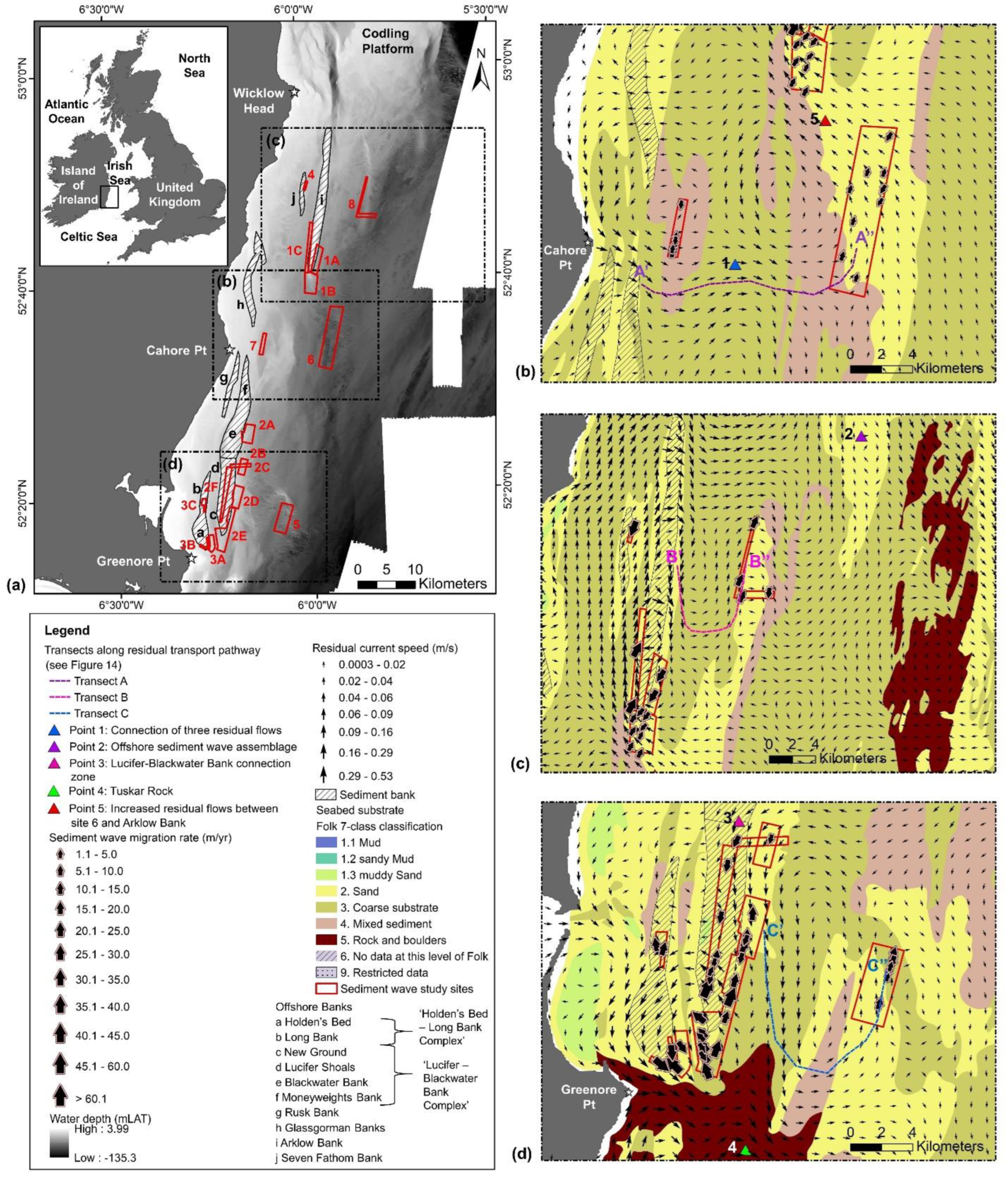
2. Regional Setting
3. Materials and Methods
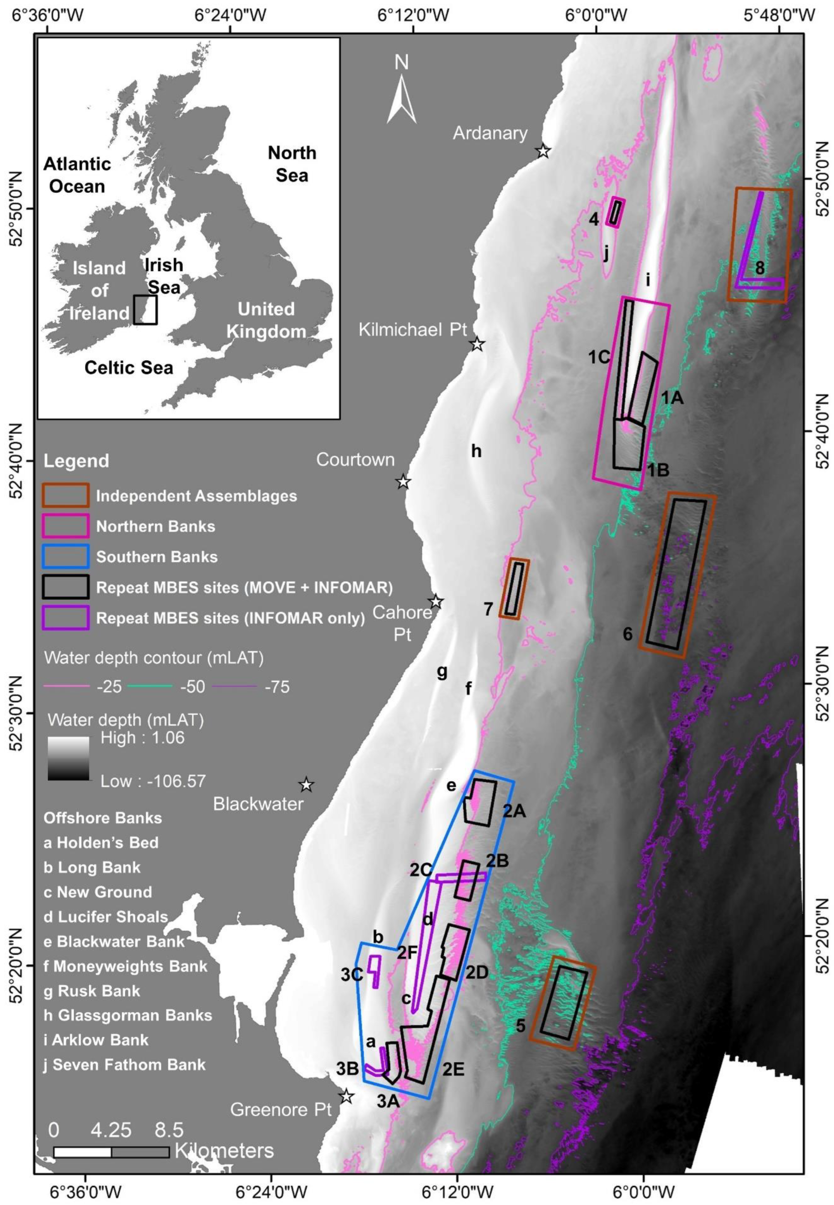
3.1. Multibeam Echo Sounder Data Acquisition and Processing
3.2. Sediment Wave Analysis
3.2.1. Sediment Wave Geometric Characteristics
3.2.2. Sand Wave Migration Direction and Rates
3.3. Sediment Samples
3.4. Hydrodynamic Modelling
3.5. Theoretical Parameters
4. Results
4.1. Sand Wave Characteristics
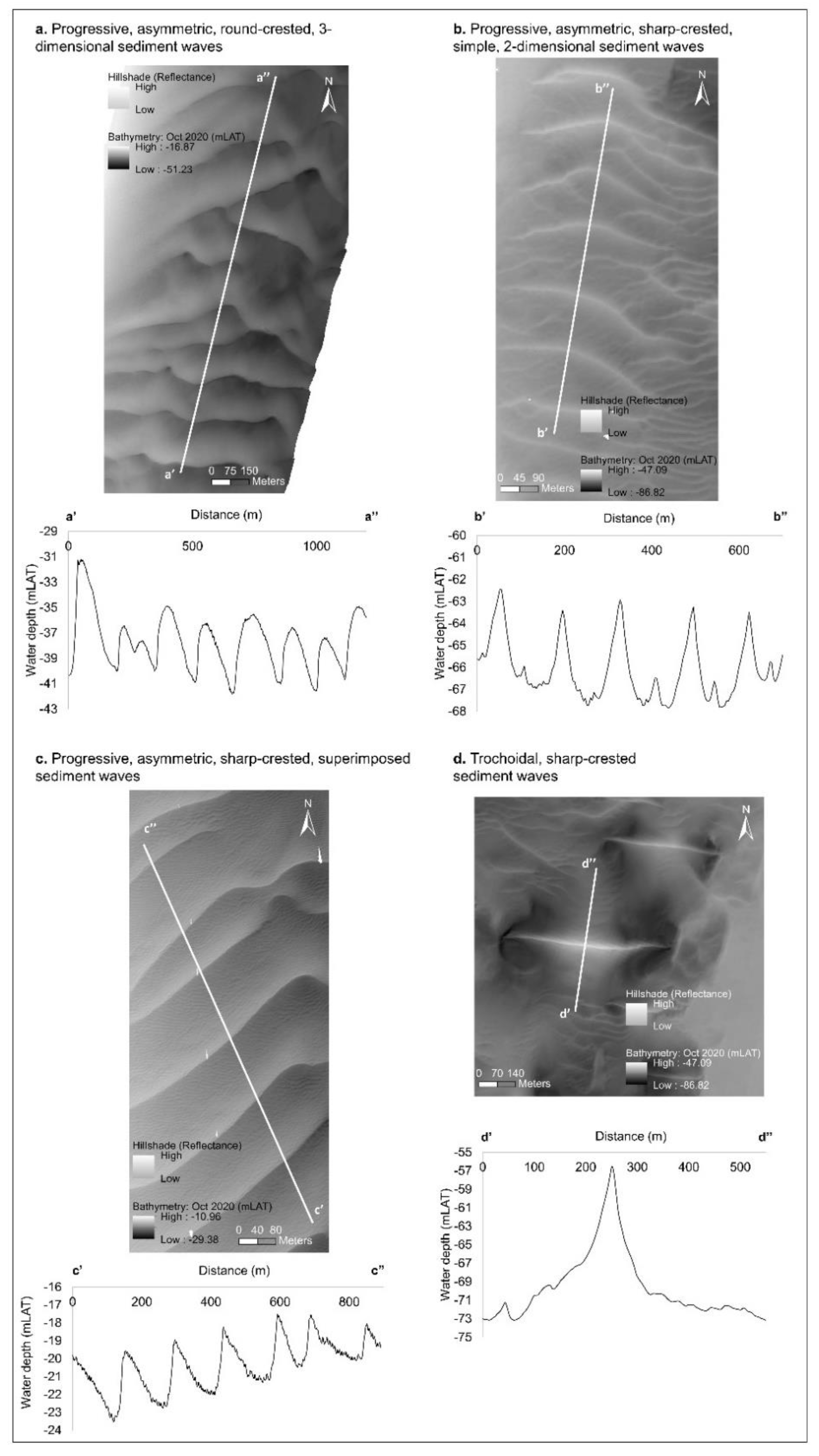
4.1.1. Sediment Wave Shape
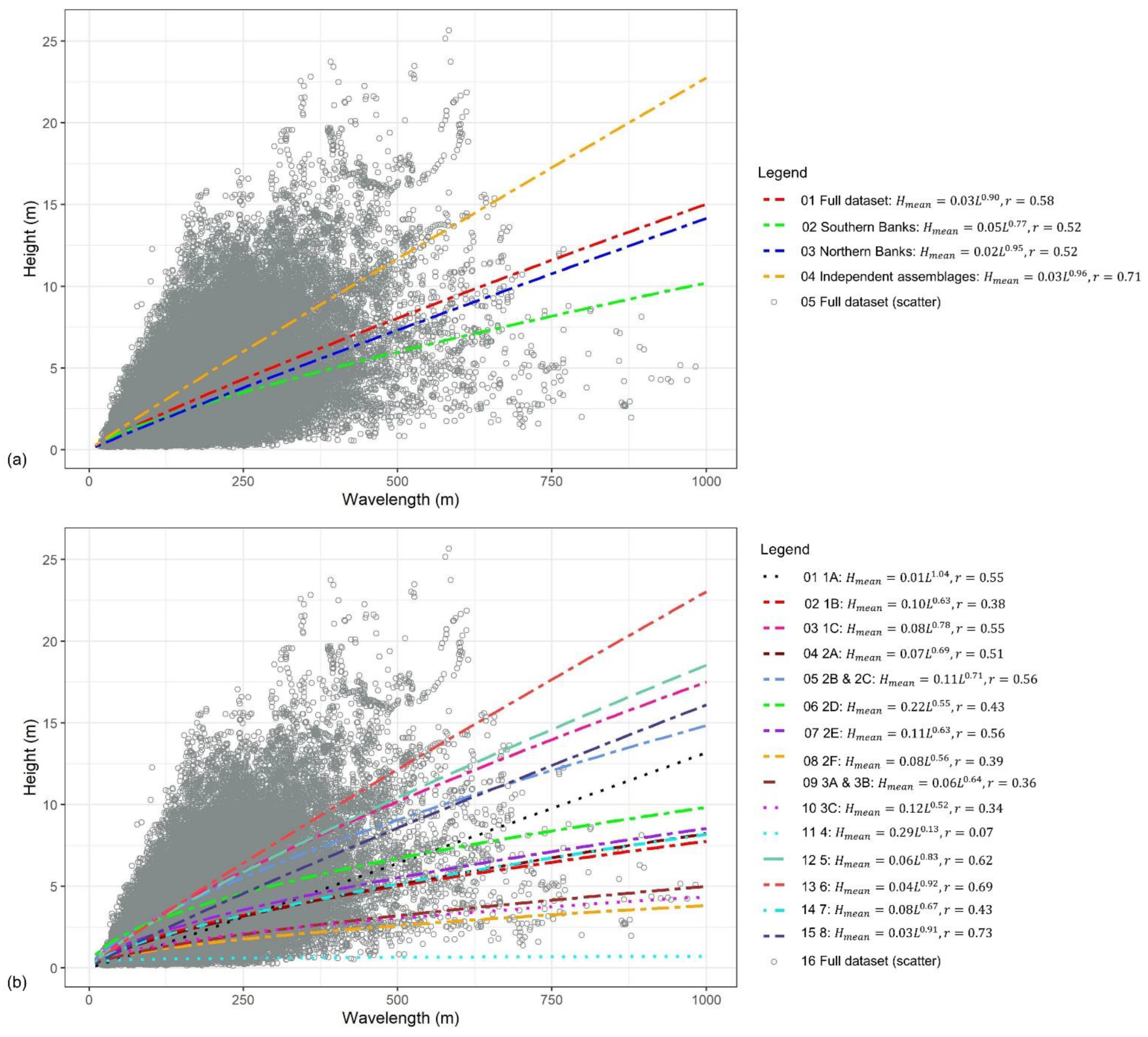
4.1.2. Sediment Wave Dimensions
4.2. Spatial and Temporal Evolution of Sediment Waves
4.2.1. Sediment Waves Associated with Arklow Bank
4.2.2. Sediment Waves Associated with Lucifer–Blackwater Bank and Holden’s Bed–Long Bank Complexes
Southern Extent of Lucifer–Blackwater Bank Complex
Lucifer–Blackwater Bank Complex Associated Waves
Long Bank Associated Sediment Waves
4.2.3. Sediment Waves Independent of Sediment Banks
Site 6
Site 5
Site 8
Site 7
4.3. Comparison between Sand Wave Characteristics, Environmental Parameters and Theory-Based Indicators
4.3.1. Correlation of Individual Sand Wave Characteristics with Environmental Parameters
4.3.2. Relationship between the Spatial Distribution of Environmental Parameters/Processes and the Occurrence of Sand Waves
5. Discussion
5.1. Connection between Average Net Sediment Wave Migration Directions and the Wider Sediment Transport Regime in the Irish Sea
5.1.1. Sediment Waves Associated with Sandbanks
5.1.2. Offshore Sediment Wave Assemblages–Sediment Supply System


5.2. Local Variations in Sand Wave Morphology
5.2.1. Singular Environmental Parameters as an Unreliable Indicator for Sediment Wave Growth
5.2.2. Geological History of the Irish Sea as a Required Background Knowledge for Present Day Sediment Wave Dynamics
5.2.3. Wave-Influence on Sediment Wave Dynamics
6. Conclusions
Supplementary Materials
Author Contributions
Funding
Data Availability Statement
Acknowledgments
Conflicts of Interest
References
- Gamberi, F.; della Valle, G.; Marani, M.; Mercorella, A.; Distefano, S.; Di Stefano, A. Tectonic Controls on Sedimentary system along the Continental Slope of the central and southeastern Tyrrhenian Sea. Ital. J. Geosci. 2019, 138, 317–332. [Google Scholar] [CrossRef]
- Short, A.D. Sediment transport around Australia–Sources, mechanisms, rates, and barrier forms. J. Coast. Res. 2010, 26, 395–402. [Google Scholar] [CrossRef]
- Zhou, J.; Wu, Z.; Zhao, D.; Guan, W.; Cao, Z.; Wang, M. Effect of topographic background on sand wave migration on the eastern Taiwan Banks. Geomorphology 2022, 398, 108030. [Google Scholar] [CrossRef]
- Zhou, J.; Wu, Z.; Zhao, D.; Guan, W.; Zhu, C.; Flemming, B. Giant sand waves on the Taiwan Banks, southern Taiwan Strait: Distribution, morphometric relationships, and hydrologic influence factors in a tide-dominated environment. Mar. Geol. 2020, 427, 106238. [Google Scholar] [CrossRef]
- Creane, S.; O’Shea, M.; Coughlan, M.; Murphy, J. The Irish Sea bed load parting zone: Is it a mid-sea hydrodynamic phenomenon or a geological theoretical concept? Estuar. Coast. Shelf Sci. 2021, 263, 107651. [Google Scholar] [CrossRef]
- Galvez, D.S.; Papenmeier, S.; Sander, L.; Bartholomä, A.; Wiltshire, K.H. Ensemble mapping as an alternative to baseline seafloor sediment mapping and monitoring. Geo-Mar. Lett. 2022, 42, 1–13. [Google Scholar] [CrossRef]
- Auguste, C.; Marsh, P.; Nader, J.R.; Penesis, I.; Cossu, R. Modelling morphological changes and migration of large sand waves in a very energetic tidal environment: Banks Strait, Australia. Energies 2021, 14, 3943. [Google Scholar] [CrossRef]
- Szczuciński, W.; Jagodziński, R.; Hanebuth, T.J.J.; Stattegger, K.; Wetzel, A.; Mitrega, M.; Unverricht, D.; van Phach, P. Modern sedimentation and sediment dispersal pattern on the continental shelf off the Mekong River delta, South China Sea. Glob. Planet. Change 2013, 110, 195–213. [Google Scholar] [CrossRef]
- Robinson, K.A.; Ramsay, K.; Lindenbaum, C.; Frost, N.; Moore, J.; Petrey, D.; Darbyshire, T. Habitat Mapping for Conservation and Management of the Southern Irish Sea (HABMAP). 2009; 5, p. 210. Available online: https://www.data.gov.uk/dataset/1baaa520-2424-46fe-bc1b-54cc0aebba44/habitat-mapping-for-conservation-and-management-of-the-southern-irish-sea-habmap (accessed on 27 September 2022).
- Wilson, B.R.; Brown, C.J.; Sameoto, J.A.; Lacharité, M.; Redden, A.M.; Gazzola, V. Mapping seafloor habitats in the Bay of Fundy to assess megafaunal assemblages associated with Modiolus modiolus beds. Estuar. Coast. Shelf Sci. 2021, 252, 107294. [Google Scholar] [CrossRef]
- Sutton, G. Irish Sea Marine Aggregate Initiative (IMAGIN); Project Synthesis Report Including: Geological Assessment, Environmental Assessment, Morphodynamic Modelling Web-based GIS System, Cost Benefit Analysis, Aggregate Resources and Markets-Wales, Marine Environment, no. 36.; Marine Institute: St. John’s, NL, Canada, 2008. [Google Scholar]
- Lewis, M.J.; Neill, S.P.; Elliott, A.J. Interannual variability of two offshore sand banks in a region of extreme tidal range. J. Coast. Res. 2015, 31, 265–275. [Google Scholar] [CrossRef]
- Phillips, M.R.; Jones, A.L. Erosion and tourism infrastructure in the coastal zone: Problems, consequences and management. Tour. Manag. 2006, 27, 517–524. [Google Scholar] [CrossRef] [Green Version]
- Distefano, S.; Gamberi, F. Preservation of Transgressive System Tract Geomorphic Elements during the Holocene Sea Level Rise in the South-Eastern Sicilian Tyrrhenian Margin. J. Mar. Sci. Eng. 2022, 10, 1013. [Google Scholar] [CrossRef]
- Morelissen, R.; Hulscher, S.J.M.H.; Knaapen, M.A.F.; Németh, A.A.; Bijker, R. Mathematical modelling of sand wave migration and the interaction with pipelines. Coast. Eng. 2003, 48, 197–209. [Google Scholar] [CrossRef]
- Yaghoobi, M.; Mazaheri, S.; Jabbari, E. Determining Natural Frequency of Free Spanning Offshore Pipelines by Considering the Seabed Soil Characteristics. J. Persian Gulf 2012, 3, 25–34. [Google Scholar]
- Sumer, B.M.; Fredsøe, J.; Christiansen, N. Scour around vertical pile in waves. J. Waterw. Port Coast. Ocean. Eng. 1992, 118, 15–31. [Google Scholar] [CrossRef]
- Whitehouse, R.J.S.; Harris, J.M.; Sutherland, J.; Rees, J. The nature of scour development and scour protection at offshore windfarm foundations. Mar. Pollut. Bull. 2011, 62, 73–88. [Google Scholar] [CrossRef] [PubMed] [Green Version]
- Department of the Environment Climate and Communications. Climate Action Plan 2021; Department of the Environment Climate and Communications: Dublin, Ireland, 2021. [Google Scholar]
- European Commission. REPowerEU: A plan to rapidly reduce dependence on Russian fossil fuels and fast forward the green transition. Press Release. 2022. Available online: https://ec.europa.eu/commission/presscorner/detail/en/IP_22_3131 (accessed on 27 September 2022).
- National Grid. ESO Pathway to 2030: A Holistic Network Design to Support Offshore Wind Deployment for Net Zero; National Grid: Warwick, UK, 2022. [Google Scholar]
- Pickering, M.D.; Wells, N.C.; Horsburgh, K.J.; Green, J.A.M. The impact of future sea-level rise on the European Shelf tides. Cont. Shelf Res. 2012, 35, 1–15. [Google Scholar] [CrossRef]
- Pickering, M.D.; Horsburgh, K.J.; Blundell, J.R.; Hirschi, J.J.M.; Nicholls, R.J.; Verlaan, M.; Wells, N.C. The impact of future sea-level rise on the global tides. Cont. Shelf Res. 2017, 142, 50–68. [Google Scholar] [CrossRef] [Green Version]
- Stow, D.A.V.; Hernández-Molina, F.J.; Llave, E.; Sayago-Gil, M.; Río, V.D.; Branson, A. Bedform-velocity matrix: The estimation of bottom current velocity from bedform observations. Geology 2009, 37, 327–330. [Google Scholar] [CrossRef]
- Dyer, K.R.; Huntley, D.A. The origin, classification and modelling of sand banks and ridges. Cont. Shelf Res. 1999, 19, 1285–1330. [Google Scholar] [CrossRef]
- Holmes, R.; Tappin, D.R. DTI Strategic Environmental Assessment Area 6, Irish Sea, Seabed and Surficial Geology and Processes. British Geological Survey Commissioned Report, CR/05/057, p. 82. 2005. Available online: http://nora.nerc.ac.uk/11259/ (accessed on 16 March 2021).
- Jackson, D.I.; Jackson, A.A.; Evans, D.J.A.; Wingfield, R.T.R.; Barnes, R.P.; Arthur, M.J. United Kingdom Offshore Regional Report: The Geology of the Irish Sea; HMSO for the British Geological Survey: London, UK, 1995. [Google Scholar]
- Johnson, M.A.; Kenyon, N.H.; Belderson, R.H.; Stride, A.H. Sand transport. In Offshore Tidal Sands: Processes and Deposits; Stride, A.H., Ed.; Chapman and Hall: London, UK, 1982; pp. 58–94. [Google Scholar] [CrossRef]
- Knaapen, M.A.F. Sandwave migration predictor based on shape information. J. Geophys. Res. Earth Surf. 2005, 110, 1–9. [Google Scholar] [CrossRef] [Green Version]
- van Landeghem, K.J.J.; Baas, J.H.; Mitchell, N.C.; Wilcockson, D.; Wheeler, A.J. Reversed sediment wave migration in the Irish Sea, NW Europe: A reappraisal of the validity of geometry-based predictive modelling and assumptions. Mar. Geol. 2012, 295, 95–112. [Google Scholar] [CrossRef]
- Nemeth, A.; Hulscher, S.J.M.H.; de Vriend, H.J. Offshore sand wave dynamics, engineering problems and future solutions. Pipeline Gas. J. 2003, 230, 67–69. [Google Scholar]
- Couldrey, A.J.; Benson, T.; Knaapen, M.A.F.; Marten, K.V.; Whitehouse, R.J.S. Morphological evolution of a barchan dune migrating past an offshore wind farm foundation. Earth Surf. Process. Landf. 2020, 45, 2884–2896. [Google Scholar] [CrossRef]
- Park, H.; Vincent, C.E. Evolution of Scroby Sands in the East Anglian coast, UK. J. Coast. Res. 2007, 868–873. Available online: http://www.jstor.org/stable/26481705 (accessed on 4 October 2022).
- Schmitt, T.; Mitchell, N.C.; Ramsay, T.S. Use of swath bathymetry in the investigation of sand dune geometry and migration around a near shore ‘banner’ tidal sandbank. Geol. Soc. Spec. Publ. 2007, 274, 53–64. [Google Scholar] [CrossRef] [Green Version]
- Caston, V.N.D. Linear sand banks in the southern North Sea. Sedimentology 1972, 18, 63–78. [Google Scholar] [CrossRef]
- Kenyon, N.H.; Cooper, B. Sand Banks, Sand Transport and Offshore Wind Farms: DTI SEA 6 Technical Report; ABPmer for Department of Trade and Industry: London, UK, 2005. [Google Scholar]
- Leenders, S.; Damveld, J.H.; Schouten, J.; Hoekstra, R.; Roetert, T.J.; Borsje, B.W. Numerical modelling of the migration direction of tidal sand waves over sand banks. Coast. Eng. 2021, 163, 103790. [Google Scholar] [CrossRef]
- Horrillo-Caraballo, J.M.; Yin, Y.; Fairley, I.; Karunarathna, H.; Masters, I.; Reeve, D.E. A comprehensive study of the tides around the Welsh coastal waters. Estuar. Coast. Shelf Sci. 2021, 254, 107326. [Google Scholar] [CrossRef]
- van Landeghem, K.J.J.; Uehara, K.; Wheeler, A.J.; Mitchell, N.C.; Scourse, J.D. Post-glacial sediment dynamics in the Irish Sea and sediment wave morphology: Data-model comparisons. Cont. Shelf Res. 2009, 29, 1723–1736. [Google Scholar] [CrossRef]
- EMODnet Bathymetry Consortium, EMODnet Digital Bathymetry (DTM 2020). 2020. Available online: https://sextant.ifremer.fr/record/bb6a87dd-e579-4036-abe1-e649cea9881a/ (accessed on 12 June 2021).
- EMODnet Geology, Seabed Substrates. 2019. Available online: https://www.emodnet-geology.eu/data-products/seabed-substrates/ (accessed on 25 June 2021).
- Cataño-Lopera, Y.A.; García, M.H. Geometry and migration characteristics of bedforms under waves and currents. Part 1: Sandwave morphodynamics. Coast. Eng. 2006, 53, 767–780. [Google Scholar] [CrossRef]
- Xu, J.P.; Wong, F.L.; Kvitek, R.; Smith, D.P.; Paull, C.K. Sandwave migration in Monterey Submarine Canyon, Central California. Mar. Geol. 2008, 248, 193–212. [Google Scholar] [CrossRef]
- Dobson, M.R.; Evans, W.E.; James, K.H. The sediment on the floor of the southern Irish Sea. Mar. Geol. 1971, 11, 27–69. [Google Scholar] [CrossRef]
- Damen, J.M.; van Dijk, T.A.G.P.; Hulscher, S.J.M.H. Spatially Varying Environmental Properties Controlling Observed Sand Wave Morphology. J. Geophys. Res. Earth Surf. 2018, 123, 262–280. [Google Scholar] [CrossRef] [Green Version]
- Ashley, G.M. Classification of large-scale subaqueous bedforms: A new look at an old problem; SEPM bedforms and bedding structures. J. Sediment. Petrol. 1990, 60, 160–172. [Google Scholar] [CrossRef]
- Flemming, B.W. Zur klassifikation subaquatischer, strömungstransversaler Transportkörper. Boch. Geol. Und. Geotech. Arb. 1988, 29, 93–97. [Google Scholar]
- Flemming, B.W. The role of grain size, water depth and flow velocity as scaling factors controlling the size of subaqueous dunes. Mar. Sandwave Dyn. 2000, 154, 55–60. [Google Scholar]
- Kubo, Y.; Soh, W.; Machiyama, H.; Tokuyama, H. Bedforms produced by the Kuroshio Current passing over the northern Izu Ridge. Geo-Mar. Lett. 2004, 24, 1–7. [Google Scholar] [CrossRef]
- Blondeaux, P.; Vittori, G. A parameterization of the wavelength of tidal dunes. Earth Surf. Process. Landf. 2011, 36, 1152–1161. [Google Scholar] [CrossRef]
- van Santen, R.B.; de Swart, H.E.; van Dijk, T.A.G.P. Sensitivity of tidal sand wavelength to environmental parameters: A combined data analysis and modelling approach. Cont. Shelf Res. 2011, 31, 966–978. [Google Scholar] [CrossRef]
- Yalin, M.S. Geometrical properties of sand wave. J. Hydraul. Div. 1964, 90, 105–119. [Google Scholar] [CrossRef]
- van der Veen, H.H.; Hulscher, S.J.M.H.; Knaapen, M.A.F. Grain size dependency in the occurrence of sand waves. Ocean. Dyn. 2006, 56, 228–234. [Google Scholar] [CrossRef]
- Franzetti, M.; le Roy, P.; Delacourt, C.; Garlan, T.; Cancouët, R.; Sukhovich, A.; Deschamps, A. Giant dune morphologies and dynamics in a deep continental shelf environment: Example of the banc du four (Western Brittany, France). Mar. Geol. 2013, 346, 17–30. [Google Scholar] [CrossRef] [Green Version]
- Bartholdy, J.; Bartholomae, A.; Flemming, B.W. Grain-size control of large compound flow-transverse bedforms in a tidal inlet of the Danish Wadden Sea. Mar. Geol. 2002, 188, 391–413. [Google Scholar] [CrossRef]
- van Landeghem, K.J.J.; Wheeler, A.J.; Mitchell, N.C.; Sutton, G. Variations in sediment wave dimensions across the tidally dominated Irish Sea, NW Europe. Mar. Geol. 2009, 263, 108–119. [Google Scholar] [CrossRef]
- Hulscher, S.J.M.H. Tidal-induced large-scale regular bed form patterns in a three-dimensional shallow water model. J. Geophys. Res. Ocean. 1996, 101, 20727–20744. [Google Scholar] [CrossRef]
- Blondeaux, P.; Vittori, G. Formation of tidal sand waves: Effects of the spring-neap cycle. J. Geophys. Res. Ocean. 2010, 115, 1–7. [Google Scholar] [CrossRef]
- Campmans, G.H.P.; Roos, P.C.; de Vriend, H.J.; Hulscher, S.J.M.H. The Influence of Storms on Sand Wave Evolution: A Nonlinear Idealized Modeling Approach. J. Geophys. Res. Earth Surf. 2018, 123, 2070–2086. [Google Scholar] [CrossRef] [Green Version]
- Borsje, B.W.; Kranenburg, W.M.; Roos, P.C.; Matthieu, J.; Hulscher, S.J.M.H. The role of suspended load transport in the occurrence of tidal sand waves. J. Geophys. Res. Earth Surf. 2014, 119, 701–716. [Google Scholar] [CrossRef] [Green Version]
- Ernstsen, V.B.; Noormets, R.; Winter, C.; Hebbeln, D.; Bartholomä, A.; Flemming, B.W.; Bartholdy, J. Development of subaqueous barchanoid-shaped dunes due to lateral grain size variability in a tidal inlet channel of the Danish Wadden Sea. J. Geophys. Res. Earth Surf. 2005, 110, 1–13. [Google Scholar] [CrossRef]
- Francken, F.; Stanislas, W.; Parker, R.; Taverniers, E. Factors influencing subaqueous dunes in the Scheldt Estuary. Geo-Mar. Lett. 2004, 24, 14–21. [Google Scholar] [CrossRef]
- Dalrymple, R.W.; Knight, R.J.; Lambiase, J.J. Bedforms and their hydraulic stability relationships in a tidal environment, Bay of Fundy, Canada. Nature 1978, 275, 100–104. [Google Scholar] [CrossRef]
- Coughlan, M.; Guerrini, M.; Creane, S.; O’Shea, M.; Ward, S.L.; van Landeghem, K.J.J.; Murphy, J.; Doherty, P. A new seabed mobility index for the Irish Sea: Modelling seabed shear stress and classifying sediment mobilisation to help predict erosion, deposition, and sediment distribution. Cont. Shelf Res. 2021, 229, 104574. [Google Scholar] [CrossRef]
- Tappin, D.R.; Chadwick, R.A.; Jackson, A.A.; Wingfield, R.T.R.; Smith, N.J.P. United Kingdom Offshore Regional Report: The Geology of Cardigan Bay and the Bristol Channel; HMSO for the British Geological Survey: London, UK, 1994. [Google Scholar]
- Wheeler, A.J.; Walshe, J.; Sutton, G.D. Geological appraisal of the Kish, Burford, Bray and Fraser Banks, Outer Dublin Bay Area. In Marine Resources Series; Marine Institute: Dublin, Ireland, 2000. [Google Scholar]
- Kozachenko, M.; Fletcher, R.; Sutton, G.; Monteys, X.; van Landeghem, K.; Wheeler, A.; Lassoued, Y.; Cooper, A.; Nicoll, C. A Geological Appraisal of Marine Aggregate Resources in the Southern Irish Sea; Technical Report Produced for the Irish Sea Marine Aggregates Initiative (IMAGIN) Project Funded under the INTERREG IIIA Community Initiative Programme 2000–2006; University College Cork: Ireland, 2008. [Google Scholar]
- Ward, S.L.; Neill, S.P.; van Landeghem, K.J.J.; Scourse, J.D. Classifying seabed sediment type using simulated tidal-induced bed shear stress. Mar. Geol. 2015, 367, 94–104. [Google Scholar] [CrossRef]
- Coughlan, M.; Long, M.; Doherty, P. Geological and geotechnical constraints in the Irish Sea for offshore renewable energy. J. Maps 2020, 16, 420–431. [Google Scholar] [CrossRef]
- Hanna, J.E.; Cooper, J.A.G. Mesoscale Morphological Changes on Linear, Nearshore Sandbanks, Co. Wexford, SE Ireland. J. Coast. Res. 2002, 36, 356–364. [Google Scholar] [CrossRef] [Green Version]
- Panigrahi, J.K.; Ananth, P.N.; Umesh, P.A. Coastal morphological modeling to assess the dynamics of Arklow Bank, Ireland. Int. J. Sediment. Res. 2009, 24, 299–314. [Google Scholar] [CrossRef]
- Walbridge, S.; Slocum, N.; Pobuda, M.; Wright, D.J. Unified Geomorphological Analysis Workflows with Benthic Terrain Modeler. Geosciences 2018, 8, 94. [Google Scholar] [CrossRef] [Green Version]
- Jasiewicz, J.; Stepinski, T.F. Geomorphons-a pattern recognition approach to classification and mapping of landforms. Geomorphology 2013, 182, 147–156. [Google Scholar] [CrossRef]
- Summers, G.; Lim, A.; Wheeler, A.J. A scalable, supervised classification of seabed sediment waves using an object-based image analysis approach. Remote Sens. 2021, 13, 2317. [Google Scholar] [CrossRef]
- van Dijk, T.A.G.P.; Lindenbergh, R.C.; Egberts, P.J.P. Separating bathymetric data representing multiscale rhythmic bed forms: A geostatistical and spectral method compared. J. Geophys. Res. Earth Surf. 2008, 113, 1–16. [Google Scholar] [CrossRef]
- Duffy, G.P. Patterns of morphometric parameters in a large bedform field: Development and application of a tool for automated bedform morphometry. Ir. J. Earth Sci. 2012, 30, 31–39. [Google Scholar] [CrossRef]
- van der Mark, C.F.; Blom, A. A New and Widely Applicable Tool for Determining the Geometric Properties of Bedforms; Report number: CE&M Research Report 2007R-003/WEM-002; University of Twente, Faculty of Engineering Technology: Enschede, The Netherlands, 2007. [Google Scholar] [CrossRef]
- Wang, L.; Yu, Q.; Zhang, Y.; Flemming, B.W.; Wang, Y.; Gao, S. An automated procedure to calculate the morphological parameters of superimposed rhythmic bedforms. Earth Surf. Process. Landf. 2020, 45, 3496–3509. [Google Scholar] [CrossRef]
- Evans, W.; Benetti, S.; Sacchetti, F.; Jackson, D.W.T.; Dunlop, P.; Monteys, X. Bedforms on the northwest Irish Shelf: Indication of modern active sediment transport and over printing of paleo-glacial sedimentary deposits. J. Maps 2015, 11, 561–574. [Google Scholar] [CrossRef] [Green Version]
- Berne, S.; Castaing, P.; le Drezen, E.; Lericolais, G. Morphology, internal structure, and reversal of asymmetry of large subtidal dunes in the entrance to Gironde Estuary (France). J. Sediment. Petrol. 1993, 63, 780–793. [Google Scholar] [CrossRef]
- di Stefano, M.; Mayer, L.A. An automatic procedure for the quantitative characterization of submarine bedforms. Geosciences 2018, 8, 28. [Google Scholar] [CrossRef] [Green Version]
- Dove, D.; Bradwell, T.; Carter, G.; Cotterill, C.; Gafeira Goncalves, J.; Green, S.; Krabbendam, M.; Mellett, C.; Stevenson, A.; Stewart, H.; et al. Seabed Geomorphology: A Two-Part Classification System; Marine Geoscience Programme. Open Report OR/16/001; British Geological Survey: Nottingham, UK, 2016. [Google Scholar]
- Kaklamanos, J.; Elmy, K. geotech: Geotechnical Engineering. R Package version 1.0, R: A Language and Environment for Statistical Computing. 2016. Available online: http://www.r-project.org/ (accessed on 4 October 2022).
- DHI Group MIKE 21 Toolbox: User Guide; DHI Group: Brisbane, QLD, Australia, 2017.
- DHI Group MIKE 21 Flow Model: Hydrodynamic Module User Guide; DHI Group: Brisbane, QLD, Australia, 2017.
- Shields, A. Anwendung der Aehnlichkeitsmechanik und der Turbulenzforschung auf die Geschiebebewegung. Preussischen Versuchsanstalt für Wasserbau. Ph.D. Thesis, Technical University Berlin, Berlin, Germany, 1936. [Google Scholar]
- Evans, J.D. Straightforward Statistics for the Behavioral Sciences; Brooks/Cole Publishing: Pacific Grove, CA, 1996. [Google Scholar]
- Huthnance, J.M. On one mechanism forming linear sand banks. Estuar. Coast. Shelf Sci. 1982, 14, 79–99. [Google Scholar] [CrossRef]
- Hulscher, S.J.M.H.; de Swart, H.E.; de Vriend, H.J. The generation of offshore tidal sand banks and sand waves. Cont. Shelf Res. 1993, 13, 1183–1204. [Google Scholar] [CrossRef] [Green Version]
- Fairley, I.; Masters, I.; Karunarathna, H. Numerical modelling of storm and surge events on offshore sandbank. Mar. Geol. 2016, 371, 106–119. [Google Scholar] [CrossRef] [Green Version]
- McCarroll, R.J.; Masselink, G.; Valiente, N.G.; Wiggins, M.; Scott, T.; Conley, D.C.; King, E.V. Impact of a headland-associated sandbank on shoreline dynamics. Geomorphology 2020, 355, 107065. [Google Scholar] [CrossRef]
- Pingree, R.D. The formation of the Shambles and other banks by tidal stirring of the sea. J. Mar. Biol. Assoc. United Kingd. 1978, 58, 211–226. [Google Scholar] [CrossRef] [Green Version]
- Bastos, A.; Collins, M.; Kenyon, N. Water and sediment movement around a coastal headland: Portland Bill, southern UK. Ocean. Dyn. 2003, 53, 309–321. [Google Scholar] [CrossRef]
- Berthot, A.; Pattiaratchi, C. Mechanisms for the formation of headland-associated linear sandbanks. Cont. Shelf Res. 2006, 26, 987–1004. [Google Scholar] [CrossRef]
- Li, M.Z.; Shaw, J.; Todd, B.J.; Kostylev, V.E.; Wu, Y. Sediment transport and development of banner banks and sandwaves in an extreme tidal system: Upper Bay of Fundy, Canada. Cont. Shelf Res. 2014, 83, 86–107. [Google Scholar] [CrossRef]
- Wentworth, C.K. A Scale of Grade and Class Terms for Clastic Sediments. J. Geol. 1922, 30, 377–392. [Google Scholar] [CrossRef]
- Neill, S.P.; Couch, S.J. Impact of Tidal Energy Converter (TEC) Array Operation on Sediment Dynamics. In Proceedings of the 9th European Wave and Tidal Energy Conference (EWTEC), Southampton, UK, 5–9 September 2011. [Google Scholar]
- Uehara, K.; Scourse, J.D.; Horsburgh, K.J.; Lambeck, K.; Purcell, A.P. Tidal evolution of the northwest European shelf seas from the Last Glacial Maximum to the present. J. Geophys. Res. Ocean. 2006, 111, 1–15. [Google Scholar] [CrossRef]
- O’Shea, M.P. Monitoring and Modelling the Morphodynamic Evolution of a Breached Barrier Beach System,” University College Cork. 2015. Available online: https://cora.ucc.ie/handle/10468/3359 (accessed on 15 May 2021).
- Colosimo, I.; de Vet, P.L.M.; van Maren, D.S.; Reniers, A.J.H.M.; Winterwerp, J.C.; van Prooijen, B.C. The impact of wind on flow and sediment transport over intertidal flats. J. Mar. Sci. Eng. 2020, 8, 910. [Google Scholar] [CrossRef]
- Daniell, J.J. Bedload parting in western Torres Strait, northern Australia. Cont. Shelf Res. 2015, 93, 58–69. [Google Scholar] [CrossRef]
- Giardino, A.; Monbaliu, J. Wave effects on the morphodynamic evolution of an offshore sand bank. J. Coast. Res. SI 2010, 51, 127–140. [Google Scholar] [CrossRef]
- Idier, D.; Ehrhold, A.; Garlan, T. Morphodynamique d’une dune sous-marine du détroit du pas de Calais. Comptes. Rendus Geosci. 2002, 334, 1079–1085. [Google Scholar] [CrossRef]
- Mitchell, N.C.; Jerrett, R.; Langman, R. Dynamics and stratigraphy of a tidal sand ridge in the Bristol Channel (Nash Sands banner bank) from repeated high-resolution multibeam echo-sounder surveys. Sedimentology 2022, 69, 1051–1082. [Google Scholar] [CrossRef]
- van Dijk, T.A.G.P.; Kleinhans, M.G. Processes controlling the dynamics of compound sand waves in the North Sea, Netherlands. J. Geophys. Res. Earth Surf. 2005, 110, 1–15. [Google Scholar] [CrossRef]


| INFOMAR Bathymetry Datasets | Mobility of Sand Waves and Sediment Banks (MOVE) Bathymetry Datasets | |||||||||
|---|---|---|---|---|---|---|---|---|---|---|
| Year Collected | 2009 | 2011 | 2012 | 2015 | 2016 | 2017 | 2020 (Sep) | 2020 (Oct) | 2021 (Mar) | |
| Offshore Survey Codes | CV09_03 | KRY11_02 CV11_03 | CV12_02 CV12_01 | KRY15_03 | KRY16_03 GEO16_03 KRY16_02 | LIR17_01 KRY17_02 | CV20010 | CV20035 | CV21035 | |
| Spatial resolution (m) | 2 | 2 5 | 2 5 | 2 | 2 | 2 | 1 | 1 | 1 | |
| Sites | 1A | |||||||||
| 1B | ||||||||||
| 1C | ||||||||||
| 2A | ||||||||||
| 2B | ||||||||||
| 2C | ||||||||||
| 2D | ||||||||||
| 2E | ||||||||||
| 2F | ||||||||||
| 3A | ||||||||||
| 3B | ||||||||||
| 3C | ||||||||||
| 4 | ||||||||||
| 5 | ||||||||||
| 6 | ||||||||||
| 7 | ||||||||||
| 8 | ||||||||||
| Sediment Wave Classification | Height (m) | Wavelength (m) |
|---|---|---|
| Small | 0.04–0.25 | 0.6–5 |
| Medium | 0.25–0.44 | 5–10 |
| Large | 0.44–2.8 | 10–100 |
| Very large | >2.8 | >100 |
| Site | Wave Height (m) | Wave Length (WL) (m) | Left WL (m) | Right WL (m) | Asymmetry | Steepness | Average Lee Slope Angle (°) | Water Depth (mLAT) | D50 (mm) | |
|---|---|---|---|---|---|---|---|---|---|---|
| 7 | mean | 2.1 | 114.5 | 65.1 | 49.4 | 0.12 | 0.019 | 3.0 | 30.2 | 0.3 |
| max | 5.2 | 355.0 | 213.0 | 241.0 | 0.72 | 0.053 | 9.3 | 32.5 | 0.5 | |
| min | 0.3 | 43.0 | 10.0 | 14.0 | −0.82 | 0.002 | 0.3 | 27.5 | 0.2 | |
| 2A | mean | 2.4 | 142.2 | 60.8 | 81.4 | −0.14 | 0.018 | 2.9 | 30.2 | 0.4 |
| max | 7.5 | 474.0 | 343.0 | 337.0 | 0.82 | 0.060 | 16.1 | 38.8 | 0.8 | |
| min | 0.2 | 22.0 | 4.0 | 7.0 | −0.92 | 0.001 | 0.0 | 18.8 | 0.2 | |
| 2B and 2C | mean | 4.0 | 150.2 | 90.3 | 59.9 | 0.18 | 0.027 | 4.6 | 26.3 | 0.6 |
| max | 11.7 | 494.0 | 446.0 | 280.0 | 0.82 | 0.069 | 14.2 | 38.1 | 2.2 | |
| min | 0.6 | 30.0 | 5.9 | 12.0 | −0.87 | 0.002 | 0.5 | 13.1 | 0.3 | |
| 2D | mean | 4.7 | 215.1 | 114.4 | 100.6 | 0.06 | 0.023 | 3.8 | 25.3 | 1.2 |
| max | 11.7 | 813.0 | 620.0 | 617.1 | 0.84 | 0.085 | 11.6 | 44.9 | 1.9 | |
| min | 0.7 | 59.0 | 9.0 | 11.9 | −0.89 | 0.002 | 0.4 | 11.6 | 0.4 | |
| 2E | mean | 2.9 | 157.4 | 76.4 | 81.1 | −0.04 | 0.021 | 3.3 | 25.4 | 1.1 |
| max | 12.3 | 983.0 | 842.0 | 883.0 | 0.91 | 0.071 | 16.0 | 38.5 | 2.6 | |
| min | 0.4 | 28.3 | 5.0 | 4.0 | −0.90 | 0.001 | 0.3 | 8.2 | 0.3 | |
| 3A and 3B | mean | 1.5 | 126.1 | 67.6 | 58.5 | 0.04 | 0.013 | 2.1 | 20.2 | 0.8 |
| max | 6.3 | 281.0 | 239.0 | 224.1 | 0.83 | 0.063 | 11.9 | 29.2 | 1.5 | |
| min | 0.2 | 30.0 | 4.0 | 7.0 | −0.91 | 0.001 | 0.2 | 9.3 | 0.3 | |
| 1A | mean | 3.0 | 140.2 | 56.3 | 83.9 | −0.19 | 0.022 | 4.1 | 34.7 | 0.8 |
| max | 15.2 | 421.0 | 310.0 | 335.0 | 0.88 | 0.083 | 27.3 | 52.2 | 5.0 | |
| min | 0.2 | 28.0 | 5.0 | 4.0 | −0.92 | 0.001 | 0.1 | 15.8 | 0.3 | |
| 1B | mean | 4.7 | 165.4 | 80.5 | 84.9 | −0.02 | 0.029 | 4.7 | 38.0 | 0.3 |
| max | 18.1 | 581.0 | 442.0 | 481.0 | 0.84 | 0.092 | 18.0 | 51.1 | 0.9 | |
| min | 0.6 | 33.0 | 9.9 | 10.9 | −0.89 | 0.003 | 0.2 | 19.1 | 0.1 | |
| 1C | mean | 2.3 | 123.5 | 56.6 | 66.9 | −0.06 | 0.020 | 3.2 | 26.1 | 0.3 |
| max | 7.5 | 422.1 | 242.1 | 338.0 | 0.91 | 0.082 | 15.6 | 39.7 | 0.8 | |
| min | 0.2 | 26.0 | 6.0 | 4.0 | −0.87 | 0.001 | 0.0 | 8.5 | 0.1 | |
| 4 | mean | 0.6 | 124.8 | 63.9 | 60.9 | 0.02 | 0.005 | 0.9 | 28.7 | 0.4 |
| max | 1.2 | 291.0 | 240.0 | 229.0 | 0.70 | 0.016 | 3.2 | 29.7 | 0.7 | |
| min | 0.1 | 50.0 | 13.0 | 12.0 | −0.65 | 0.001 | 0.1 | 27.1 | 0.3 | |
| 5 | mean | 6.1 | 216.7 | 106.5 | 110.2 | −0.02 | 0.029 | 4.8 | 57.9 | 0.6 |
| max | 23.5 | 681.0 | 505.0 | 576.1 | 0.86 | 0.088 | 17.4 | 72.9 | 2.3 | |
| min | 0.9 | 52.0 | 4.9 | 13.0 | −0.91 | 0.002 | 0.5 | 36.6 | 0.2 | |
| 6 | mean | 4.7 | 163.7 | 77.2 | 86.5 | −0.05 | 0.030 | 4.8 | 65.9 | 1.3 |
| max | 25.7 | 614.0 | 428.1 | 460.1 | 0.80 | 0.120 | 23.0 | 83.0 | 5.0 | |
| min | 0.4 | 34.0 | 5.9 | 9.9 | −0.90 | 0.002 | 0.5 | 52.8 | 0.3 | |
| 3C | mean | 1.4 | 101.8 | 51.5 | 50.3 | 0.00 | 0.015 | 2.5 | 18.7 | 1.0 |
| max | 3.7 | 313.0 | 196.0 | 213.0 | 0.77 | 0.044 | 8.5 | 26.8 | 2.8 | |
| min | 0.2 | 29.0 | 3.0 | 9.0 | −0.87 | 0.001 | 0.0 | 10.4 | 0.8 | |
| 2F | mean | 1.5 | 174.9 | 62.9 | 112.0 | −0.27 | 0.009 | 1.8 | 11.2 | 0.8 |
| max | 4.4 | 599.0 | 336.0 | 391.0 | 0.73 | 0.043 | 8.0 | 14.2 | 1.1 | |
| min | 0.2 | 45.0 | 9.0 | 22.0 | −0.92 | 0.001 | 0.1 | 7.8 | 0.3 | |
| 8 | mean | 3.4 | 159.8 | 93.6 | 66.3 | 0.11 | 0.022 | 3.7 | 53.5 | 0.5 |
| max | 10.2 | 478.0 | 365.1 | 303.0 | 0.83 | 0.068 | 15.4 | 72.0 | 1.0 | |
| min | 0.1 | 17.0 | 3.0 | 5.0 | −0.87 | 0.001 | 0.3 | 40.0 | 0.3 |
| Dataset | Power Regression Equation | Correlation Coefficient () | Correlation Description | |
|---|---|---|---|---|
| Full dataset | 0.33 | 0.58 | Moderate positive | |
| Southern Banks | 0.27 | 0.52 | Moderate positive | |
| Northern Banks | 0.28 | 0.52 | Moderate positive | |
| Independent Assemblages | 0.50 | 0.71 | Strong positive | |
| 8 | 0.53 | 0.73 | Strong positive | |
| 2F | 0.15 | 0.39 | Weak positive | |
| 3C | 0.12 | 0.34 | Weak positive | |
| 6 | 0.48 | 0.69 | Strong positive | |
| 5 | 0.38 | 0.62 | Strong positive | |
| 4 | 0 | 0.07 | Very weak positive or no association | |
| 1C | 0.30 | 0.55 | Moderate positive | |
| 1B | 0.14 | 0.38 | Weak positive | |
| 1A | 0.30 | 0.55 | Moderate positive | |
| 3A and 3B | 0.13 | 0.36 | Weak positive | |
| 2E | 0.31 | 0.56 | Moderate positive | |
| 2D | 0.19 | 0.43 | Moderate positive | |
| 2B and 2C | 0.31 | 0.56 | Moderate positive | |
| 2A | 0.26 | 0.51 | Moderate positive | |
| 7 | 0.19 | 0.43 | Moderate positive |
Publisher’s Note: MDPI stays neutral with regard to jurisdictional claims in published maps and institutional affiliations. |
© 2022 by the authors. Licensee MDPI, Basel, Switzerland. This article is an open access article distributed under the terms and conditions of the Creative Commons Attribution (CC BY) license (https://creativecommons.org/licenses/by/4.0/).
Share and Cite
Creane, S.; Coughlan, M.; O’Shea, M.; Murphy, J. Development and Dynamics of Sediment Waves in a Complex Morphological and Tidal Dominant System: Southern Irish Sea. Geosciences 2022, 12, 431. https://doi.org/10.3390/geosciences12120431
Creane S, Coughlan M, O’Shea M, Murphy J. Development and Dynamics of Sediment Waves in a Complex Morphological and Tidal Dominant System: Southern Irish Sea. Geosciences. 2022; 12(12):431. https://doi.org/10.3390/geosciences12120431
Chicago/Turabian StyleCreane, Shauna, Mark Coughlan, Michael O’Shea, and Jimmy Murphy. 2022. "Development and Dynamics of Sediment Waves in a Complex Morphological and Tidal Dominant System: Southern Irish Sea" Geosciences 12, no. 12: 431. https://doi.org/10.3390/geosciences12120431
APA StyleCreane, S., Coughlan, M., O’Shea, M., & Murphy, J. (2022). Development and Dynamics of Sediment Waves in a Complex Morphological and Tidal Dominant System: Southern Irish Sea. Geosciences, 12(12), 431. https://doi.org/10.3390/geosciences12120431