

Application of Non-Reflective Boundary Conditions in Three-Dimensional Numerical Simulations of Free-Surface Flow Problems

 ,
,  ,
,
Abstract

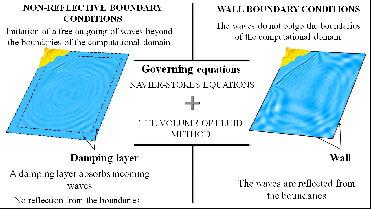
1. Introduction
2. Governing Equations
2.1. Mathematical Model
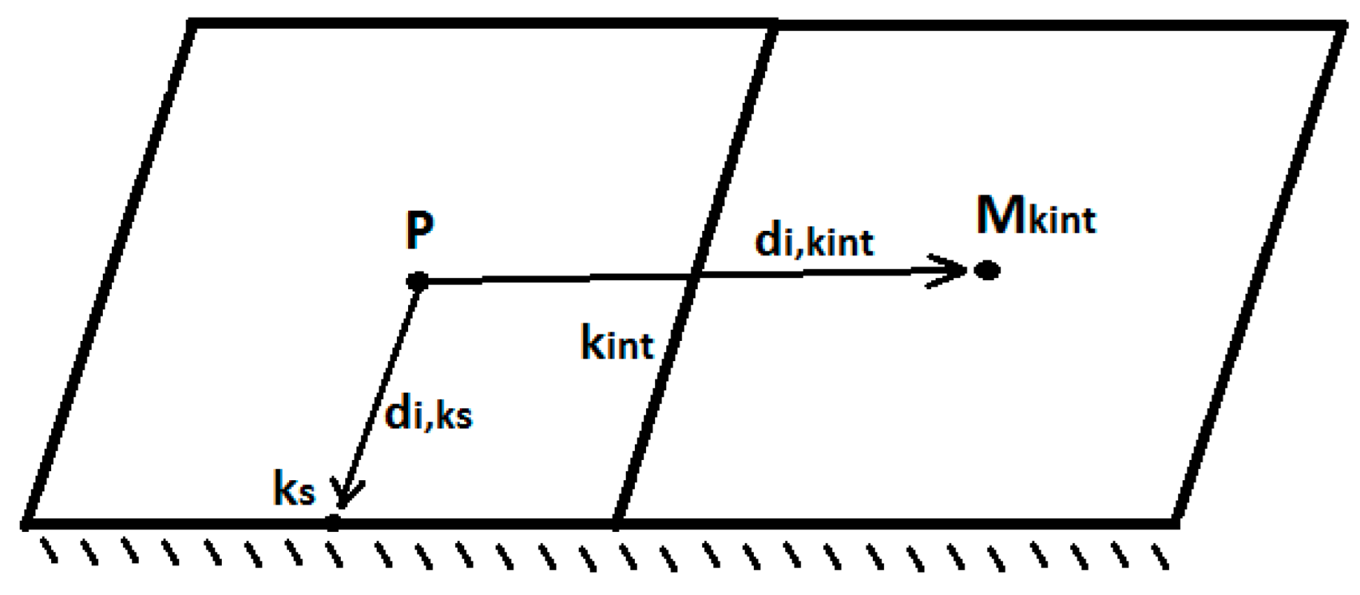
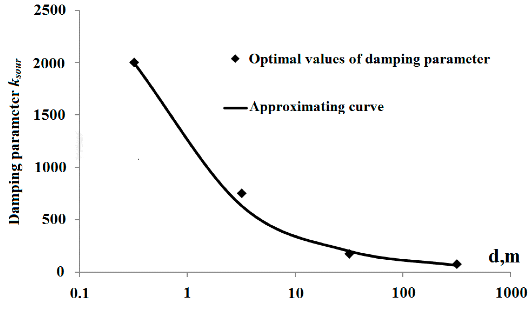
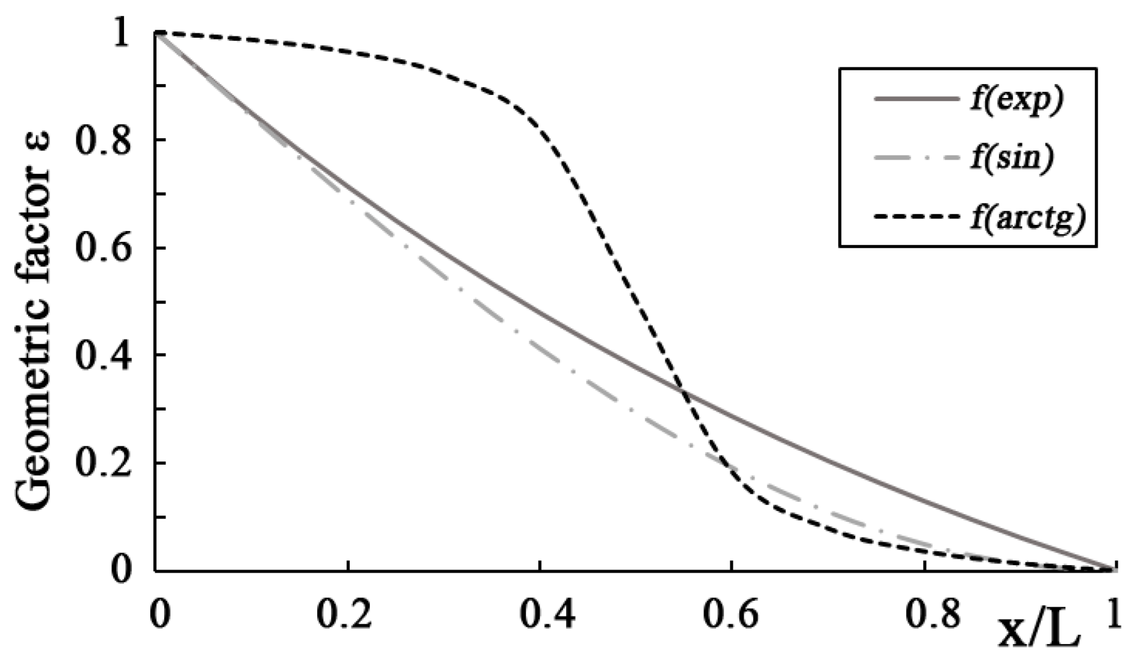
2.2. Damping Method
3. Numerical Experiments. Bathymetry-Aware Simulation of Tsunami Waves Traveling across a Real Water Body
4. Conclusions
Author Contributions
Funding
Data Availability Statement
Conflicts of Interest
References
- Fürst, J.; Musil, J. Development of non-reflective boundary conditions for free-surface flows. In Proceedings of the Topical Problems of Fluid Mechanics, Prague, Czech Republic, 21–23 February 2018. [Google Scholar]
- Mani, A. On the reflectivity of sponge zones in compressible flow simulations. In Annual Research Brief; Ames Research Center: Mountain View, VA, USA, 2010. [Google Scholar]
- Salvesen, H.-C.; Teigland, R. Non-reflecting boundary conditions applicable to general purpose CFD simulators. Int. J. Numer. Meth. Fluids 1998, 28, 523–540. [Google Scholar] [CrossRef]
- Giles, M. Non-Reflecting Boundary Conditions for the Euler Equations; Computational Fluid Dynamics Laboratory, Department of Aeronautics and Astronautics, Massachusetts Institute of Technology: Cambridge, MA, USA, 1988. [Google Scholar]
- Granet, V.; Vermorel, O.; Leonard, T.; Gicquel, L.; Poinsot, T. Comparison of nonreflecting outlet boundary conditions for compressible solvers on unstructured grids. AIAA J. 2010, 48, 2348–2364. [Google Scholar] [CrossRef]
- Dorodnitsyn, L.V. Non-reflecting boundary conditions for the gas dynamics equations systems. J. Comput. Math. Math. Phys. 2002, 42, 522–549. (In Russian) [Google Scholar]
- Givoli, D.; Neta, B. High-order nonreflecting boundary conditions for the dispersive shallow water equations. J. Comput. Appl. Math. 2003, 158, 49–60. [Google Scholar] [CrossRef]
- Carmigniani, R.A.; Violeau, D. Optimal sponge layer for water waves numerical models. Ocean Eng. 2018, 163, 169–182. [Google Scholar] [CrossRef]
- Wei, G. The Sponge Layer Method in FLOW-3D; Flow Science, Inc.: Santa Fe, NM, USA, 2015. [Google Scholar]
- Peric, R.; Abdel-Maksoud, M. Reliable Damping of Free Surface Waves in Numerical Simulations. Ship Technol. Res. 2016, 63, 1–13. [Google Scholar] [CrossRef]
- Hsu, T.W.; Ou, S.H.; Yang, B.D.; Tseng, I.F. On the damping coefficients of sponge layer in Boussinesq equations. Wave Motion 2005, 41, 45–57. [Google Scholar] [CrossRef]
- Wang, D.; Dong, S. A discussion of numerical wave absorption using sponge layer methods. Ocean Eng. 2022, 247, 110732. [Google Scholar] [CrossRef]
- Torregrosa, A.J.; Fajardo, P.; Gil, A.; Navarro, R. Development of Non-Reflecting Boundary Condition for Application in 3D Computational Fluid Dynamics Codes. Eng. Appl. Comput. Fluid Mech. 2012, 6, 447–460. [Google Scholar] [CrossRef]
- Kar, S.K.; Turco, R.P. Formulation of a Lateral Sponge Layer for Limited-Area Shallow-Water Models and an Extension for the Vertically Stratified Case. Mon. Wea. Rev. 1994, 123, 1542–1559. [Google Scholar] [CrossRef]
- Kozelkov, A.S. The Numerical Technique for the Landslide Tsunami Simulations Based on Navier-Stokes Equations. J. Appl. Mech. Tech. Phys. 2017, 58, 1192–1210. [Google Scholar] [CrossRef]
- Kozelkov, A.S.; Efremov, V.R.; Kurkin, A.A.; Pelinovsky, E.N.; Tarasova, N.V.; Strelets, D.Y. Three dimensional numerical simulation of tsunami waves based on the Navier-Stokes equations. Sci. Tsunami Hazards 2017, 36, 183–196. [Google Scholar]
- Kozelkov, A.S.; Lashkin, S.V.; Efremov, V.R.; Volkov, K.N.; Tsibereva, Y.A.; Tarasova, N.V. An implicit algorithm of solving Navier–Stokes equations to simulate flows in anisotropic porous media. Comput. Fluids 2018, 160, 164–174. [Google Scholar] [CrossRef]
- Kozelkov, A.S.; Kurkin, A.A.; Sharipova, I.L.; Kurulin, V.V.; Pelinovsky, E.N.; Tyatyushkina, E.S.; Meleshkina, D.P.; Lashkin, S.V.; Tarasova, N.V. Minimal basis tasks for validation of methods of calculation of flows with free surfaces. Trans. R.E. Alekseev NSTU 2015, 2, 49–69. [Google Scholar]
- Tyatyushkina, E.S.; Kozelkov, A.S.; Kurkin, A.A.; Pelinovsky, E.N.; Kurulin, V.V.; Plygunova, K.S.; Utkin, D.A. Verification of the LOGOS Software Package for Tsunami Simulations. Geosciences 2020, 10, 385. [Google Scholar] [CrossRef]
- Efremov, V.R.; Kozelkov, A.S.; Kornev, A.V.; Kurkin, A.A.; Kurulin, V.V.; Strelets, D.Y.; Tarasova, N.V. Method for taking into account gravity in free-surface flow simulation. Comput. Math. Math. Phys. 2017, 57, 1720–1733. [Google Scholar] [CrossRef]
- Chen, Z.J.; Przekwas, A.J. A coupled pressure-based computational method for incompressible/compressible flows. J. Comp. Phys. 2010, 229, 9150–9165. [Google Scholar] [CrossRef]
- Hrabry, A.I.; Zaitsev, D.K.; Smirnov, Y.M. Numerical simulation of currents with free surface based on VOF method. Trans. Krylov State Res. Cent. 2013, 78, 53–64. (In Russian) [Google Scholar]
- Roache, P. Computational Fluid Dynamics; Mir: Moscow, Russian, 1980; 618p, (Translated into Russian). [Google Scholar]
- Jasak, H. Error Analysis and Estimation for the Finite Volume Method with Applications to Fluid Flows. Ph.D. Thesis, Department of Mechanical Engineering, Imperial College of Science, London, UK, 1996. [Google Scholar]
- Jasak, H.; Weller, H.G.; Gosman, A.D. High resolution NVD differencing scheme for arbitrarily unstructured meshes. Int. J. Numer. Methods Fluids 1999, 31, 431–449. [Google Scholar] [CrossRef]
- Gaskell, P.H. Curvature-compensated convective-transport—SMART, A new boundedness-preserving transport algorithm. Int. J. Numer. Methods Fluids 1988, 8, 617–641. [Google Scholar] [CrossRef]
- Muzaferija, S.; Peric, M.; Sames, P.; Schelin, T. A two-fluid Navier-Stokes solver to simulate water entry. In Proceedings of the 22nd Symposium of Naval Hydrodynamics, Washington, DC, USA, 9–14 August 1998. [Google Scholar]
- Waclawczyk, T.; Koronowicz, T. Remarks on prediction of wave drag using VOF method with interface capturing approach. Arch. Civ. Mech. Eng. 2008, 8, 5–14. [Google Scholar] [CrossRef]
- Volkov, K.N.; Kozelkov, A.S.; Lashkin, S.V.; Tarasova, N.V.; Yalozo, A.V. A Parallel Implementation of the Algebraic Multigrid Method for Solving Problems in Dynamics of Viscous Incompressible Fluid. Comput. Math. Math. Phys. 2017, 57, 2030–2046. [Google Scholar] [CrossRef]


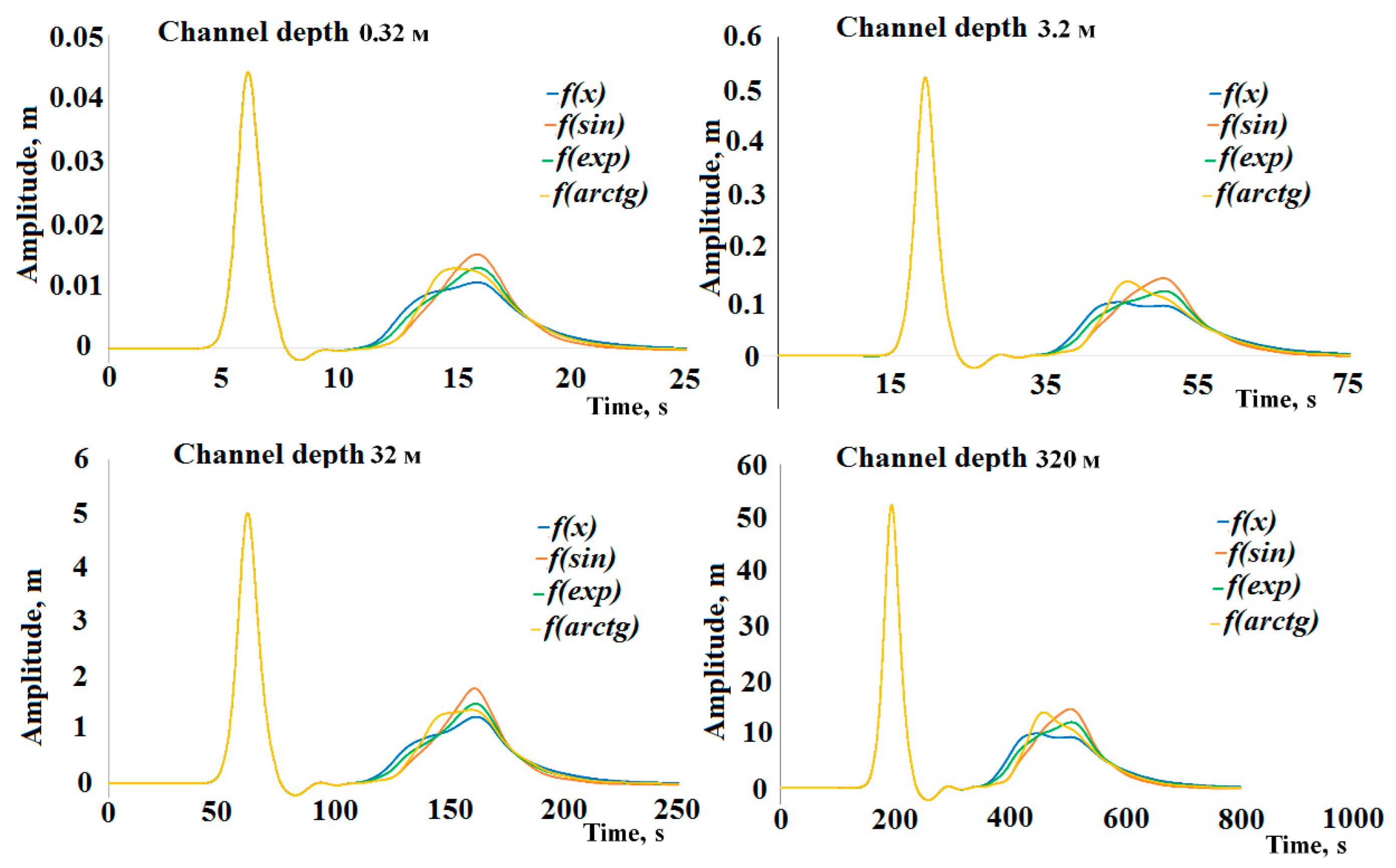
| Case | Channel Depth, m | Channel Length, mm | Wave Height, m | Wavelength, m | L, m |
|---|---|---|---|---|---|
| 1 | 0.32 | 23 | 0.064 | 4.24 | 4 |
| 2 | 3.2 | 230 | 0.64 | 40.24 | 40 |
| 3 | 32 | 2300 | 6.4 | 402.4 | 400 |
| 4 | 320 | 23,000 | 64 | 4024 | 4000 |
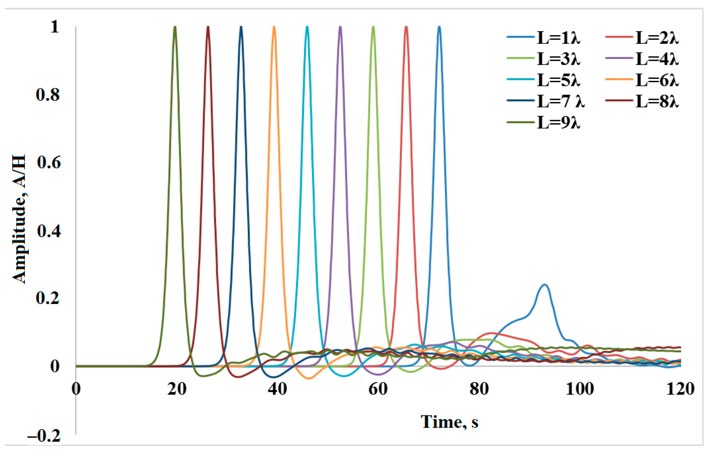
| Width of Damping Zone | Amplitude Relationship between Reflected and Incident Waves, % |
|---|---|
| 1λ | 23.8 |
| 2λ | 9.7 |
| 3λ | 7.8 |
| 4λ | 6.5 |
| 5λ | 5.3 |
| 6λ | 4.6 |
| 7λ | 4.5 |
| 8λ | 4.4 |
| 9λ | 4.4 |
Publisher’s Note: MDPI stays neutral with regard to jurisdictional claims in published maps and institutional affiliations. |
© 2022 by the authors. Licensee MDPI, Basel, Switzerland. This article is an open access article distributed under the terms and conditions of the Creative Commons Attribution (CC BY) license (https://creativecommons.org/licenses/by/4.0/).
Share and Cite
Kozelkov, A.; Kurkin, A.; Utkin, D.; Tyatyushkina, E.; Kurulin, V.; Strelets, D. Application of Non-Reflective Boundary Conditions in Three-Dimensional Numerical Simulations of Free-Surface Flow Problems. Geosciences 2022, 12, 427. https://doi.org/10.3390/geosciences12110427
Kozelkov A, Kurkin A, Utkin D, Tyatyushkina E, Kurulin V, Strelets D. Application of Non-Reflective Boundary Conditions in Three-Dimensional Numerical Simulations of Free-Surface Flow Problems. Geosciences. 2022; 12(11):427. https://doi.org/10.3390/geosciences12110427
Chicago/Turabian StyleKozelkov, Andrey, Andrey Kurkin, Dmitry Utkin, Elena Tyatyushkina, Vadim Kurulin, and Dmitry Strelets. 2022. "Application of Non-Reflective Boundary Conditions in Three-Dimensional Numerical Simulations of Free-Surface Flow Problems" Geosciences 12, no. 11: 427. https://doi.org/10.3390/geosciences12110427
APA StyleKozelkov, A., Kurkin, A., Utkin, D., Tyatyushkina, E., Kurulin, V., & Strelets, D. (2022). Application of Non-Reflective Boundary Conditions in Three-Dimensional Numerical Simulations of Free-Surface Flow Problems. Geosciences, 12(11), 427. https://doi.org/10.3390/geosciences12110427