

Imaging Arctic Permafrost: Modeling for Choice of Geophysical Methods

 , ,
, ,  ,
,
Abstract
1. Introduction
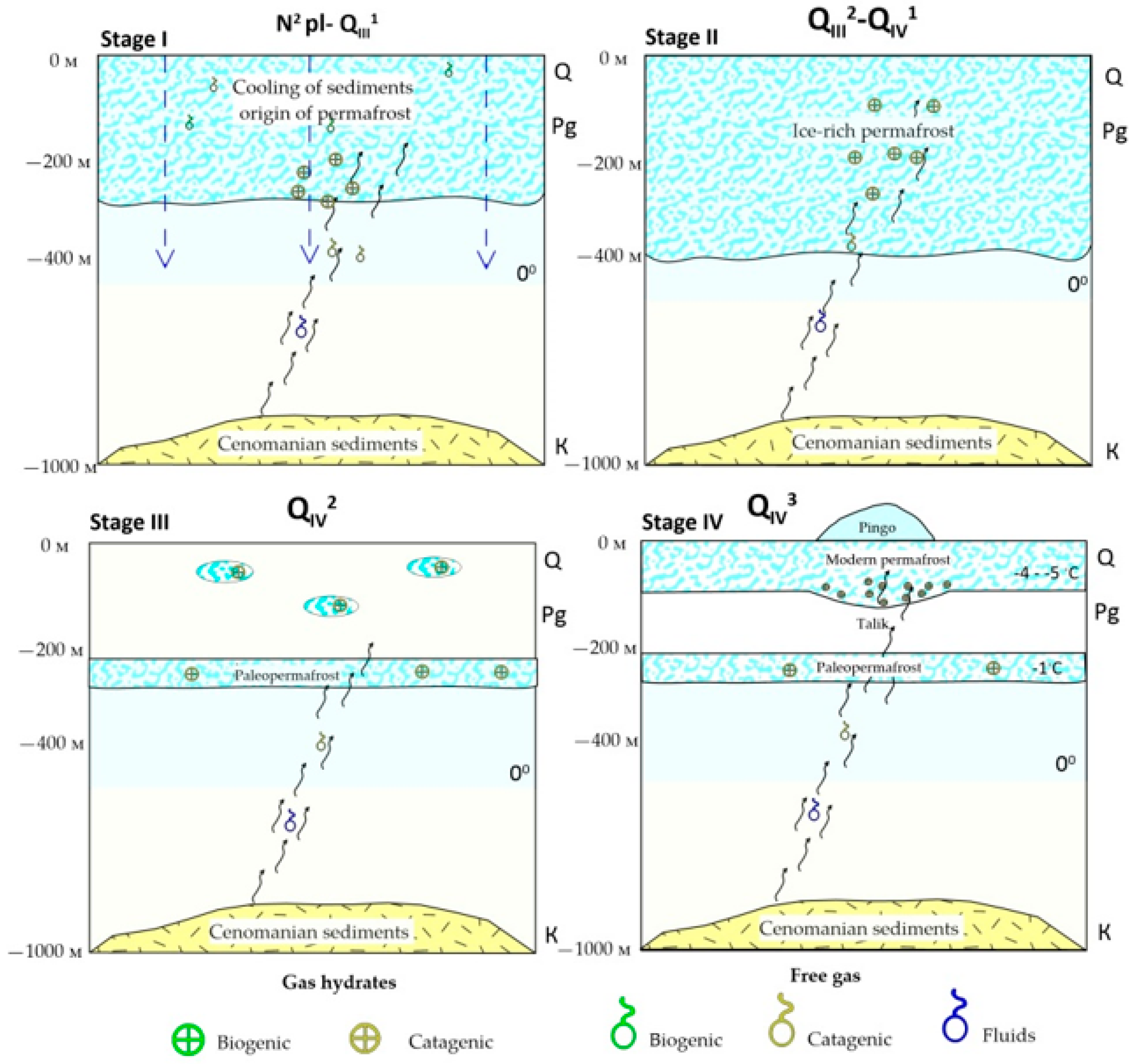
2. History of Permafrost in Northern West Siberia
3. Geophysical–Geological Model of Northern West Siberia
4. Methods
- Common mid-point seismic reflection profiling (CMP);
- DC electrical resistivity tomography (ERT);
- Shallow transient electromagnetic sounding (sTEM).
5. Results
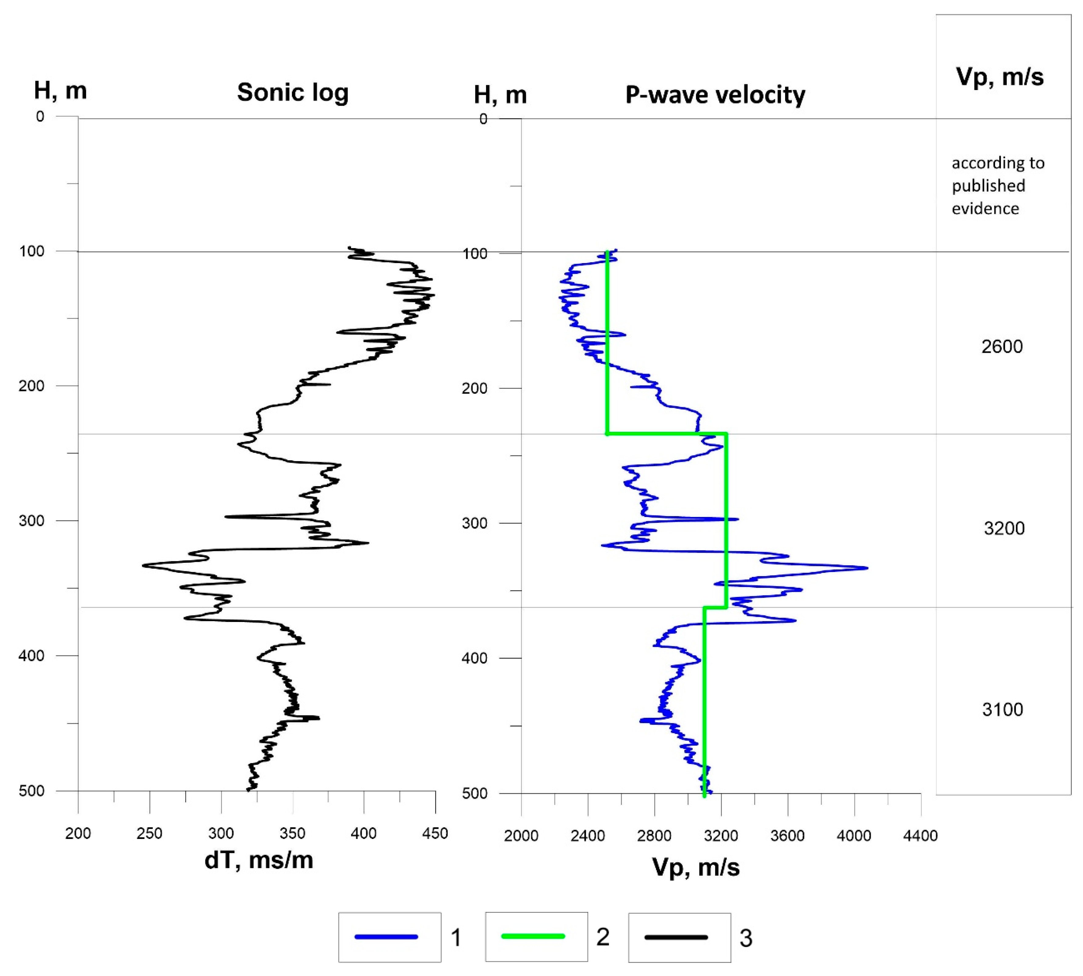
5.1. CMP Seismic Data
5.2. ERT Data
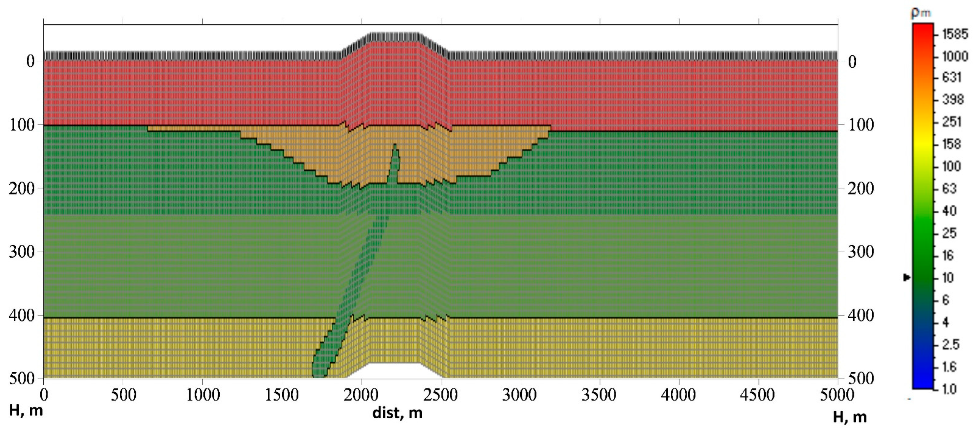
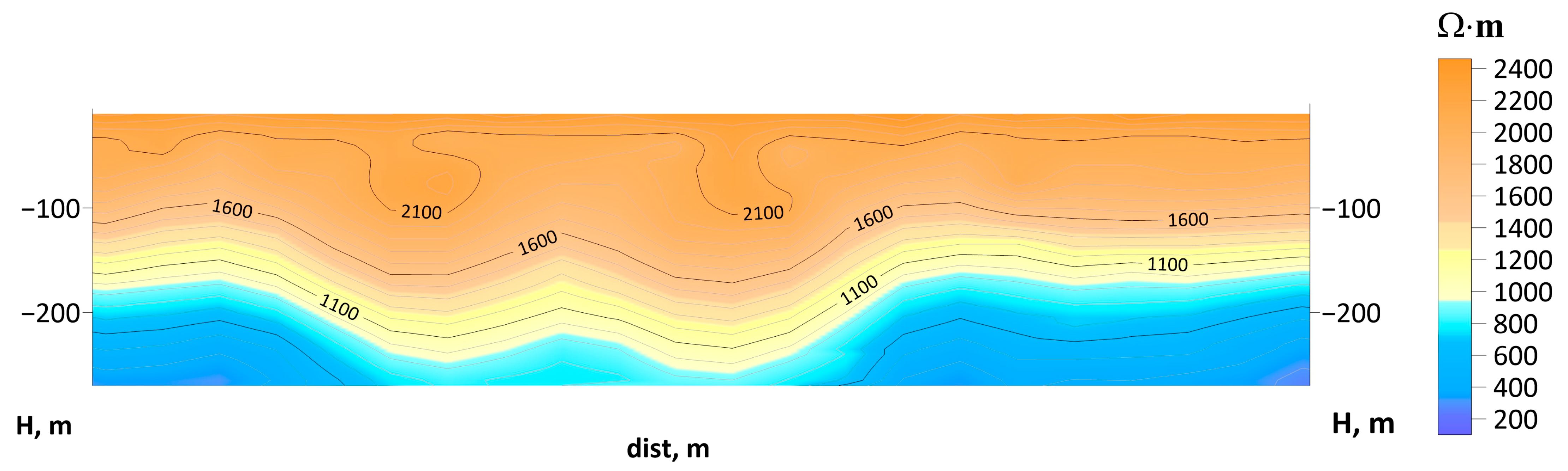
5.3. TEM Data
6. Discussion
7. Conclusions
Author Contributions
Funding
Data Availability Statement
Acknowledgments
Conflicts of Interest
References
- Ershov, E.D. Geocryology of the USSR Territory; West Siberia, Nedra: Moscow, Russia, 1989; p. 454. (In Russian) [Google Scholar]
- Yakushev, B.C.; Perlova, E.V.; Makhonina, N.A.; Chuvilin, E.M.; Kozlova, E.V. Gas hydrates in sediments of continents and islands. Ross. Khimicheskii Zhurnal 2003, 3, 80–90. [Google Scholar]
- Yakushev, V.S. Natural Gas and Gas Hydrates in Permafrost; VNIIGAZ: Moscow, Russia, 2009; p. 192. (In Russian) [Google Scholar]
- Chuvilin, E.M.; Guryeva, M. Experimental Study of the Self-Preservation Effect of Gas Hydrates in Frozen Sediments. In Proceedings of the 9th International Conference on Permafrost, Fairbanks, Alaska, 29 June–3 July 2008; University of Alaska: Fairbanks, AK, USA, 2008; pp. 263–267. [Google Scholar]
- Chuvilin, E.M.; Buhanov, B.; Davletshina, D.; Grebenkin, S. Dissociation and self-preservation of gas hydrates in permafrost. Geosciences 2018, 8, 431. [Google Scholar] [CrossRef]
- Yakushev, V.S.; Chuvilin, E.M. Natural gas and hydrate accumulation within permafrost in Russia. Cold Reg. Sci. Technol. 2000, 31, 189–197. [Google Scholar] [CrossRef]
- Kraev, G.; Rivkina, E.; Vishnivetskaya, T.; Belonosov, A.; van Huissteden, J.; Kholodov, A.; Smirnov, A.; Kudryavtsev, A.; Teshebaeva, K.; Zamolodchikov, D. Methane in gas shows from boreholes in epigenetic permafrost of Siberian Arctic. Geosciences 2019, 9, 67. [Google Scholar] [CrossRef]
- Chuvilin, E.; Ekimova, V.; Davletshina, D.; Sokolova, N.; Bukhanov, B. Evidence of gas emissions from permafrost in the Russian Arctic. Geosciences 2020, 10, 383. [Google Scholar] [CrossRef]
- Chuvilin, E.; Sokolova, N.; Davletshina, D.; Bukhanov, B.; Stanilovskaya, J.; Badetz, C.; Spasennykh, M. Conceptual models of gas accumulation in the shallow permafrost of northern West Siberia and conditions for explosive gas emissions. Geosciences 2020, 10, 195. [Google Scholar] [CrossRef]
- Dostovalov, B.N.; Kudryavtsev, V.A. General Geocryology; Moscow University Press: Moscow, Russia, 1967; p. 443. (In Russian) [Google Scholar]
- Boikov, S.A. Resistivity Survey for Engineering Geological and Geocryological Studies of Discontinuous Permafrost; Author’s Abstract, Candidate Thesis (Geology & Mineralogy); Gosstroi SSSR: Moscow, Russia, 1973; p. 32. (in Russain) [Google Scholar]
- Bogolyubov, A.N.; Bogolyubova, N.P.; Lisitsyn, V.V.; Kurandin, N.P. Guidelines to Engineering Geophysical (Resistivity) Surveys for Construction; Stroiizdat: Moscow, Russia, 1984; p. 104. (In Russian) [Google Scholar]
- Zykov, Y.D. Geophysical Methods for Permafrost Studies; Moscow University Press: Moscow, Russia, 1999; p. 243. (In Russian) [Google Scholar]
- Yakupov, V.S. Geophysics of Permafrost Regions; Yakutsk University: Yakutsk, Russia, 2008; p. 341. (In Russian) [Google Scholar]
- Melnikov, V.P.; Skvortsov, A.G.; Malkova, G.V.; Drozdov, D.S.; Ponomareva, O.E.; Sadurtdinov, M.R.; Tsarev, A.M.; Dubrovin, V.A. Seismic studies of frozen ground in Arctic areas. Russ. Geol. Geophys. 2010, 51, 136–142. [Google Scholar] [CrossRef]
- Skvortsov, A.G.; Tsarev, A.M.; Sadurtdinov, M.R. Seismic studies of frozen ground. Earth’s Cryosphere 2011, 4, 96–98. [Google Scholar]
- Clairmont, R.; Bedle, H.; Marfurt, K.; Wang, Y. Seismic attribute analyses and attenuation applications for detecting gas hydrate presence. Geosciences 2021, 11, 450. [Google Scholar] [CrossRef]
- Tayber, Z.; Meilijson, A.; Ben-Avraham, Z.; Makovsky, Y. Methane hydrate stability and potential resource in the Levant Basin, southeastern Mediterranean Sea. Geosciences 2019, 9, 306. [Google Scholar] [CrossRef]
- Lenz, B.L.; Sawyer, D.E.; Phrampus, B.; Davenport, K.; Long, A. Seismic imaging of seafloor deformation induced by impact from large submarine landslide blocks, offshore Oregon. Geosciences 2019, 9, 10. [Google Scholar] [CrossRef]
- Bogoyavlensky, V.; Kishankov, A.; Yanchevskaya, A.; Bogoyavlensky, I. Forecast of gas hydrates distribution zones in the Arctic Ocean and adjacent offshore areas. Geosciences 2018, 8, 453. [Google Scholar] [CrossRef]
- Ostanin, I.; Anka, Z.; Di Primio, R. Role of faults in hydrocarbon leakage in the Hammerfest Basin, SW Barents Sea: Insights from seismic data and numerical modelling. Geosciences 2017, 7, 28. [Google Scholar] [CrossRef]
- Weitemeyer, K.A.; Constable, S.; Tréhu, A.M. A marine electromagnetic survey to detect gas hydrate at Hydrate Ridge, Oregon. Geophys. J. Int. 2011, 187, 45–62. [Google Scholar] [CrossRef]
- Hsu, S.-K.; Chiang, C.-W.; Evans, R.; Chen, C.-S.; Chiu, S.-D.; Wang, Y.; Chen, S.-C.; Tsai, C.-H.; Lin, S.-S. Marine controlled-source electromagnetic method used for the gas hydrate investigation in the offshore area of SW Taiwan. J. Asian Earth Sci. 2014, 92, 224–232. [Google Scholar] [CrossRef]
- Li, G.; Tang, F.; Li, C.; Lei, W.; Liu, Y. Improved detectivity for detecting gas hydrates using the weighted differential fields of the marine controlled-source electromagnetic data. J. Mar. Sci. Eng. 2022, 10, 161. [Google Scholar] [CrossRef]
- Jing, J.; Chen, K.; Deng, M.; Zhao, Q.X.; Luo, X.H.; Tu, G.-H.; Wang, M. A marine controlled-source electromagnetic survey to detect gas hydrates in the Qiongdongnan Basin, South China Sea. J. Asian Earth Sci. 2019, 171, 201–212, ISSN 1367-9120. [Google Scholar] [CrossRef]
- Wang, L.; Li, Y. Field Result of Marine Controlled-Source Electromagnetic Survey for Gas Hydrates in Northern South China Sea. In Proceedings of the 5th International Conference on Systems and Informatics (ICSAI), Nanjing, China, 10–12 November 2018; pp. 871–877. [Google Scholar] [CrossRef]
- Riedel, M.; Willoughby, E.C.; Chopra, S. (Eds.) Geophysical Characterization of Gas Hydrates, Geophysical Developments 1; Society of Exploration Geophysicists: Sidney, BC, Canada, 2010; p. 412. [Google Scholar] [CrossRef]
- Shpolyanskaya, N.A. Physiography of West Siberia. In Permafrost in West Siberia: History and Distribution Patterns; Moscow State University: Moscow, Russia, 1971; pp. 120–123. (In Russian) [Google Scholar]
- Baulin, Y.I. Permafrost in Petroleum Provinces of the USSR; Nauka: Moscow, Russia, 1985; p. 176. (In Russian) [Google Scholar]
- Drushchits, V.A.; Sadchikova, T.A.; Skolotneva, T.S. Onshore and Artcic shelf gas hydrates and Quaternary global change. Comm. Quat. 2011, 71, 124–134. [Google Scholar]
- Saks, V.N. The Quaternary History of the Soviet Arctic; Glavsevmorput: Moscow-Leningrad, Russia, 1948; p. 201. (In Russian) [Google Scholar]
- Saks, V.N. The Quaternary Period in the Soviet Arctic; NIIGA Transactions: Moscow, Leningrad, Russia, 1953; Volume 77, p. 627. (In Russian) [Google Scholar]
- Arkhipov, S.A.; Astakhov, V.I.; Volkov, I.A.; Volkova, V.S.; Panychev, V.A. Paleogeography of the West Siberian Plain in the Late Zyryanian Glacial Maximum; Nauka: Novosibirsk, Russia, 1980; p. 114. (In Russian) [Google Scholar]
- Vasilchuk, Y.K. Late Pleistocene and Holocene paleoclimates: Reconstructions from isotope data for ground ice and waters in permafrost regions. Vodn. Resur. 1990, 6, 162–170. [Google Scholar]
- Cleimenov, V.F.; Kachalov, Y.M. Subpermafrost gas accumulations in the Arctic petroleum province: Mapping methodology. In Petroleum Geology and Exploration Lines; VNIGNI: Moscow, Russia, 2003; pp. 191–202. (In Russian) [Google Scholar]
- Nezhdanov, A.A.; Novopashin, V.F.; Ogibenin, V.V. Mud volcanism in the north of Western Siberia. In TyumenNIIgiprogaz; Flat: Tyumen, Russia, 2011; pp. 74–79. (In Russian) [Google Scholar]
- Nezhdanov, A.A.; Smirnov, A.S. (Eds.) Fluid Dynamic Interpretation of Seismic Data: Student’s Manuel; TIU: Tyumen, Russia, 2021; p. 286. (In Russian) [Google Scholar]
- Buddo, I.V.; Misurkeeva, N.V.; Shelokhov, I.A.; Agafonov, Y.A.; Smirnov, A.S.; Zharikov, M.G.; Kulinchenko, A.S. Experience of 3D Transient Electromagnetics Application for Shallow and Hydrocarbon Exploration within Western Siberia. In Proceedings of the 79th EAGE Conference & Exhibition 2017, Paris, France, 12–15 June 2017. [Google Scholar] [CrossRef]
- Misyurkeeva, N.; Buddo, I.; Kraev, G.; Smirnov, A.; Nezhdanov, A.; Shelokhov, I.; Kurchatova, A.; Belonosov, A. Periglacial Landforms and Fluid Dynamics in the Permafrost Domain: A Case from the Taz Peninsula, West Siberia. Energies 2022, 15, 2794. [Google Scholar] [CrossRef]
- Misyurkeeva, N.V.; Buddo, I.V.; Agafonov, Y.A.; Smirnov, A.S.; Zharikov, M.G.; Kulinchenko, A.S. 3D TEM and sTEM results from Arctic West Siberia. In Proceedings of the Geomodel 2017, Gelendzhik, Russia, 11–14 September 2017. [Google Scholar]
- Misyurkeeva, N.; Buddo, I.; Shelokhov, I.; Smirnov, A.; Nezhdanov, A.; Agafonov, Y. The structure of permafrost in northern West Siberia: Geophysical evidence. Energies 2022, 15, 2847. [Google Scholar] [CrossRef]
- Misurkeeva, N.V.; Buddo, I.V.; Smirnov, A.S.; Shelokhov, I.A. Shallow transient electromagnetic method application to study the Yamal Peninsula Permafrost Zone. In Proceedings of the Geomodel 2020, Gelendzhik, Russia, 7–11 September 2020; pp. 1–6. [Google Scholar]
- Shelokhov, I.A. Integration of Geophysical Methods for Predicting the Near-Surface Velocity Structure; Author’s Abstract, Candidate Thesis; Institute of the Earth’s Crust: Irkutsk, Russia, 2022; p. 16. (In Russian) [Google Scholar]
- Murzina, E.V.; Pospeev, A.V.; Buddo, I.V.; Sharlov, M.V.; Seminskiy, I.K.; Misyurkeeva, N.V.; Shelohov, I.A. Capabilities of shallow-depth transient electromagnetic soundings for identification of gas-hydrate accumulations in the cryolithozone of the northern regions of Western Siberia. Earth’s Cryosphere 2022, 26, 51–62. [Google Scholar] [CrossRef]
- Chuvilin, E.M.; Perlova, E.V.; Baranov, Y.B.; Kondakov, V.V.; Osokin, A.B.; Yakushev, V.S. Structure and Properties of Permafrost in the Offshore Southern Bovanenkovskoye Gas Condensate Field; GEOS: Moscow, Russia, 2007; pp. 74–113. (In Russian) [Google Scholar]
- Chuvilin, E.M.; Davletshina, D.A.; Lupachik, M.V. Hydrate formation in frozen and thawing methane-saturated sediments. Earth’s Cryosphere 2019, 2, 50–61. [Google Scholar] [CrossRef]
- Leonov, S.A. Prospects for the Hydration Potential of the Supra-Cenomanian Deposits in Northern West Siberia; Author’s Abstract, Candidate Thesis (Geology & Mineralogy); Gazprom VNIIGAZ: Moscow, Russia, 2010; p. 24. (In Russian) [Google Scholar]
- Butler, D.K. (Ed.) Near-Surface Geophysics; SEG: Tulsa, OK, USA, 2005; p. 732. [Google Scholar]
- Yilmaz, O. Engineering Seismology; SEG: Tulsa, OK, USA, 2015; p. 954. [Google Scholar]
- Yilmaz, O. Seismic Data Processing; SEG: Tulsa, OK, USA, 1986; p. 526. [Google Scholar]
- Boganik, G.N.; Gurvich, I.I. Seismic Exploration; AIS: Tver, Russia, 2006; p. 744. (In Russian) [Google Scholar]
- Miller, R.D.; Bradford, J.H.; Holliger, K. (Eds.) Advances in Near-Surface Seismology and Ground-Penetrating Radar; SEG Geophysical Developments Series No. 15; Society of Exploration Geophysicists; American Geophysical Union; Environmental and Engineering Geophysical Society: Tulsa, OK, USA; Washington, DC, USA, 2010; p. 487. [Google Scholar]
- Bobachev, A.A.; Marchenko, M.N.; Modin, I.N.; Pervago, E.V.; Urusova, A.V.; Shevnin, V.A. Resistivity surveys in a horizontally heterogeneous earth: New approaches. Izv. RAN Fiz. Zemli 1995, 12, 79–90. [Google Scholar]
- Stefanescu, S.; Schlumberger, C.; Schlumberger, M. Sur la Distribution Électrique Potentielle autour d’Une Prise de Terre Ponctuelle Dans un Terrain à Couches Horisontales Homogènes et Isotropes. J. Phys. Radium 1930, 4, 132–140. [Google Scholar] [CrossRef]
- Khmelevskoy, V.K. Resistivity Surveys. Student’s Manual; Moscow University: Moscow, Russia, 1984; p. 422. (In Russian) [Google Scholar]
- Kalinin, A.V.; Khmelevskoy, V.K.; Vladov, M.L.; Zolotaya, L.A.; Kulnitsky, L.M.; Starovoitov, A.V.; Tokarev, M.Y.; Shalaeva, N.V. Modern georadar surveys. Razved. Okhrana Nedr. 2001, 3, 2–6. [Google Scholar]
- Vladov, M.L.; Starovoitov, A.V. Fundamentals of Ground Penetrating Radar Surveys; Moscow University Press: Moscow, Russia, 2004; p. 155. (In Russian) [Google Scholar]
- Finkelshtein, M.I.; Kutev, V.A.; Zolotarev, V.P. Near-Surface Ground Penetrating Radar Surveys for Engineering Geology; Nedra: Moscow, Russia, 1986. (In Russian) [Google Scholar]
- Buddo, I.V.; Sharlov, M.; Shelokhov, I.; Misyurkeeva, N.; Seminsky, I.; Selyaev, V.; Agafonov, Y. Applicability of transient electromagnetic surveys to permafrost imaging in Arctic West Siberia. Energies 2022, 15, 1816. [Google Scholar] [CrossRef]
- Kaufman, A.A.; Morozova, G.M. Transient Electromagnetic Soundings: Theoretical Background; Nauka: Novosibirsk, Russia, 1970; p. 123. (In Russian) [Google Scholar]
- Tabarovsky, L.A.; Epov, M.I.; Sosunov, O.G. Estimating the Resolution of Electromagnetic Surveys and Noise Attenuation; IGiG SO AN SSSR: Novosibirsk, Russia, 1985; p. 47. (In Russian) [Google Scholar]
- Vanyan, L.L. Electromagnetic Soundings; Nauchny mir: Moscow, Russia, 1997; p. 218. (In Russian) [Google Scholar]
- McNeill, J.D. Application of Transient Electromagnetic Techniques; Geonics Limited: Missasauga, ON, Canada, 1980; p. 17. [Google Scholar]
- Korolkov, Y.S. Transient Electromagnetic (TEM) Soundings for Petroleum Exploration; Nedra: Moscow, Russia, 1987; p. 117. (In Russian) [Google Scholar]
- Reynolds, J.M. An Introduction to Applied and Environmental Geophysics; John Wiley and Sons Ltd.: Chichester, UK, 1997; p. 796. [Google Scholar]
- Mogilatov, V.S. Induction Resistivity Surveys; Student’s Manual; Novosibirsk State University: Novosibirsk, Russia, 2014; p. 182. (In Russian) [Google Scholar]
- Pospeev, A.V.; Buddo, I.V.; Agafonov, Y.A.; Sharlov, M.V.; Kompaniets, S.V.; Tokareva, O.V.; Misyurkeeva, N.V.; Gomylskiy, V.V.; Surov, L.V.; Ilyin, A.I. Modern Resistivity Survey Practices; GEO Publishers: Novosibirsk, Russia, 2018; p. 231. (In Russian) [Google Scholar]
- Kozhevnikov, N.O.; Sharlov, M.V. Early-Time and Late-Time Limitations on the Performance of Near-Surface TEM Measuring Systems. In Proceedings of the Near Surface Geoscience Conference & Exhibition 2019, Hague, The Netherlands, 8–12 September 2019. [Google Scholar]
- Sharlov, M.V.; Kozhevnikov, N.O.; Pestyurin, T.N. Improving the performance of measurement systems for shallow TEM soundings. In Proceedings of the VIII Russian Seminar on Resistivity Surveys 2021., Moscow, Russia, 26 September–2 October 2021. (In Russian). [Google Scholar]
- Sharlov, M.V.; Buddo, I.V.; Misyurkeeva, N.V.; Shelokhov, I.A.; Agafonov, Y.A. Transient electromagnetic surveys for high resolution near-surface exploration: Basics and case studies. First Break 2017, 35, 63–71. [Google Scholar] [CrossRef]
- Available online: http://zond-geo.com/software/resistivity-imaging-ves/zondres2d/ (accessed on 9 October 2022).
- Agafonov, Y.A.; Pospeev, A.V.; Surov, L.V. Electromagnetic surveys in the southern Siberian craton: System for data interpretation and main uses of transient electromagnetic surveys. Prib. I Sist. Razvedochnoi Geofiz. 2006, 1, 33–36. [Google Scholar]
- Misyurkeeva, N.; Buddo, I.; Shelokhov, I.; Smirnov, A.; Agafonov, Y.; Nezhdanov, A.; Tokareva, O. The structure of the permafrost section from high-density transient electromagnetic method (TEM) data within the Yamal Peninsula. In Proceedings of the ProGREss’21 Conference, Sochi, Russia, 1–3 November 2021; pp. 1–6. [Google Scholar]
- Rybalchenko, V.V.; Trusov, A.I.; Buddo, I.V.; Abramovich, A.V.; Smirnov, A.S.; Misyurkeeva, N.V.; Shelokhov, I.A.; Otsimik, A.A.; Agafonov, Y.A.; Gorlov, I.V.; et al. Additional studies in petroleum exploration and development: From permafrost mapping to groundwater prospecting for drilling and operation of wells. Gazov. Promyshlennost 2020, 11, 20–28. [Google Scholar]


| Method | Base of Ice-Rich Permafrost | Base of Relict Permafrost Lenses with Hypothetical Gas Hydrates | Vertical Fluid Conduits |
|---|---|---|---|
| CMP | + | + | − |
| ERT | + | − | − |
| TEM | + | + | + |
Publisher’s Note: MDPI stays neutral with regard to jurisdictional claims in published maps and institutional affiliations. |
© 2022 by the authors. Licensee MDPI, Basel, Switzerland. This article is an open access article distributed under the terms and conditions of the Creative Commons Attribution (CC BY) license (https://creativecommons.org/licenses/by/4.0/).
Share and Cite
Buddo, I.; Misyurkeeva, N.; Shelokhov, I.; Chuvilin, E.; Chernikh, A.; Smirnov, A. Imaging Arctic Permafrost: Modeling for Choice of Geophysical Methods. Geosciences 2022, 12, 389. https://doi.org/10.3390/geosciences12100389
Buddo I, Misyurkeeva N, Shelokhov I, Chuvilin E, Chernikh A, Smirnov A. Imaging Arctic Permafrost: Modeling for Choice of Geophysical Methods. Geosciences. 2022; 12(10):389. https://doi.org/10.3390/geosciences12100389
Chicago/Turabian StyleBuddo, Igor, Natalya Misyurkeeva, Ivan Shelokhov, Evgeny Chuvilin, Alexey Chernikh, and Alexander Smirnov. 2022. "Imaging Arctic Permafrost: Modeling for Choice of Geophysical Methods" Geosciences 12, no. 10: 389. https://doi.org/10.3390/geosciences12100389
APA StyleBuddo, I., Misyurkeeva, N., Shelokhov, I., Chuvilin, E., Chernikh, A., & Smirnov, A. (2022). Imaging Arctic Permafrost: Modeling for Choice of Geophysical Methods. Geosciences, 12(10), 389. https://doi.org/10.3390/geosciences12100389