1. Introduction
The discovery of fossil remains of vertebrates, as well as that of other buried biogenic structures, is often an occasional event during random and time-consuming excavations across promising study sites. In addition, excavations are clearly invasive, resulting in the destruction of surveyed ground and are done or at punctual sites, or along relatively short trenches, which cannot provide complete knowledge of the spatial distribution of fossils. Important paleontological sites are often incidentally discovered during excavation activities related to the construction of infrastructures or arise in protected areas. Therefore, as for archaeological studies, prior non-invasive screening of the area is mandatory to plan only targeted trenching.
Different geophysical methods are used with varying degrees of success in many applications of Earth Science. Among the available geophysical tools, the Ground Penetrating Radar (GPR) is frequently used in geology in particular for shallow prospections requiring high resolution [
1,
2,
3,
4]. Over time, GPR has proven useful in soil studies [
5], sedimentology [
6], in fault and fracture characterization [
7,
8,
9,
10], in hydrogeology [
11,
12,
13,
14,
15,
16,
17,
18,
19], and in archeological applications [
20,
21,
22,
23].
A few studies regarding the GPR detection of fossiliferous beds and/or large fossil remains are available in literature, well summarized by [
24]. The authors report results of a GPR survey aiding the discovery of a lower Pliocene sirenian skeleton in the Arcille site close to Grosseto (Tuscany, Italy). The remains were found embedded in shallow marine siliciclastic deposits, mainly consisting of bioclastic sandstone overlain greyish mudstone [
24]. Using a 200 MHz antenna, the authors detected distinct GPR signatures, which correlate with the skeleton bones and fossiliferous beds, and encouraged the use of GPR in paleontological applications. More recently, [
25] verified, in the laboratory, the GPR resolution capability of two 1.0 GHz and 1.5 GHz frequency antennas on three biomicrite samples, for the detection of paleontological remains. Both studies report the GPR has the resolution capability to identify fragments or concentrations of fossils with a decametric-centimetric size [
24,
25], as known clearly depending on different factors (e.g., the type of antenna used, physical properties of surveyed media, the type and size of fossils). GPR was also revealed to be effective in map anomalies arising from the skeletal remains of a late Pleistocene mammoth frozen in ice [
26] at the Bering Land Bridge National Preserve in Alaska, as well as in providing tridimensional imaging of human-megafauna footprints (“ghost tracks”) at the White Sands National Monument in New Mexico (USA) [
27].
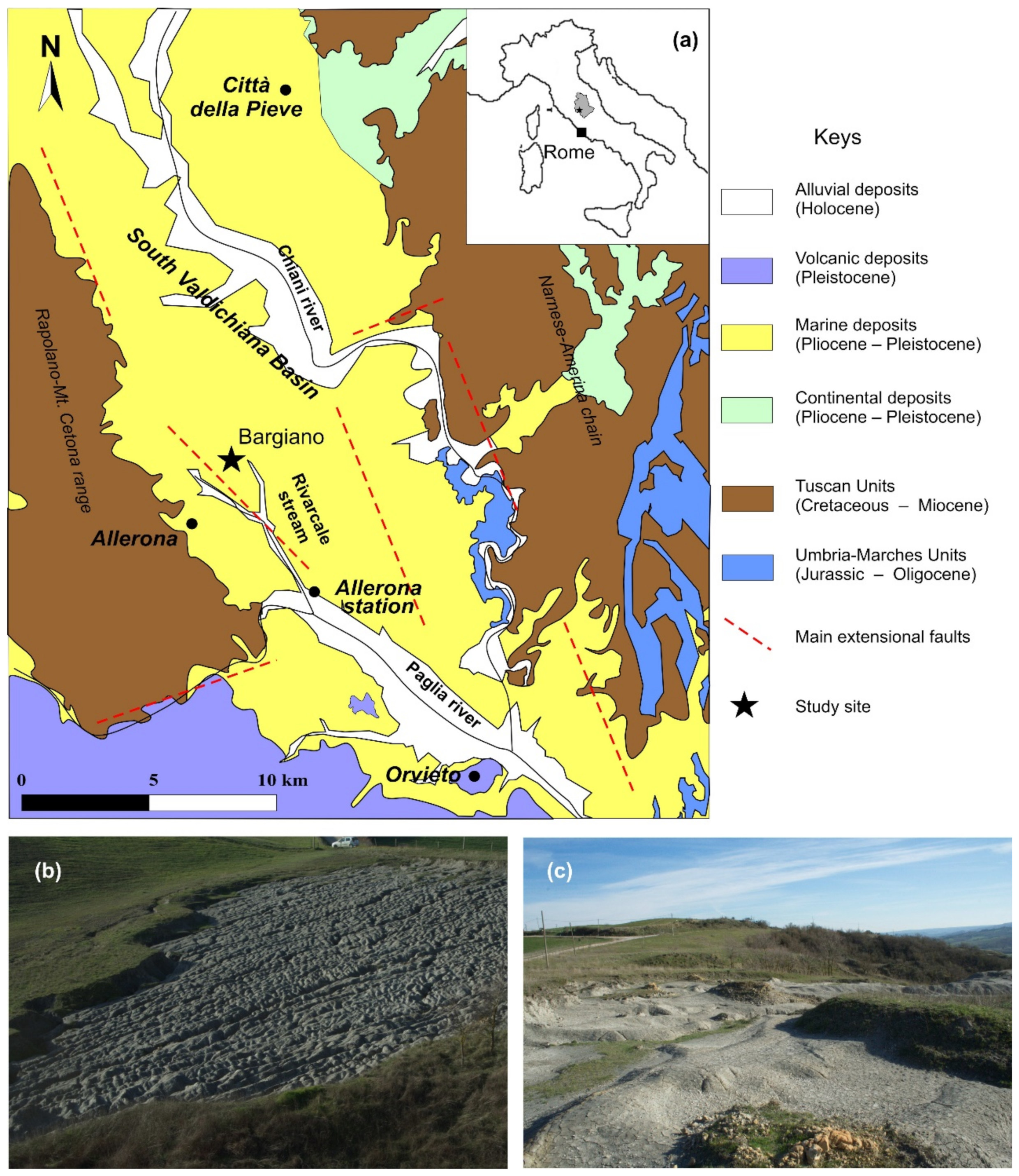
In this study, we report the results of a GPR survey carried out at the Bargiano site in central Italy. This study site is located in the vicinity of the Allerona village, in the southwestern sector of the Umbria Region (
Figure 1). Pleistocene sediments, mainly consisting of clayey/silty and clayey marine deposits, widely outcrop across the area (
Figure 1a). The site is already known in paleontological records for the exceptional first fossil report of sperm-whale cololites (
Ambergrisichnus alleronae, [
28,
29]). The Allerona area also returned, in recent years, three partially preserved whale skeletons, and the recent discovery and recovery of a fourth whale skeleton [
30]. Following the tales of the residents, which are frequently plowing and tilling the soil on the site during agricultural activities, the occurrence of such types of structures and fossils is suspected to be spread across a wider area. As for other studies, also at Bargiano, past excavations were executed mostly randomly or nearby occasional remain outcroppings after intense erosional processes. Although these fieldworks provided excellent results, they required several operators and efforts, such as staying for long working sessions excavating in the field. For these reasons, we considered a GPR survey ideal to support additional excavations and to focus the fieldwork of the paleontologists in more restricted areas. However, the Bargiano site presents severe environmental conditions for a GPR survey, due to the presence of a steep slope as well as a very irregular topographic surface. The latter is caused by pervasive gully erosion characterizing the area, which exhibits deep grooves along the maximum slope (
Figure 1b). This characteristic is strictly due to the lithology of the sedimentary deposits covering the site, mainly made by marine silty clays [
30], thus potentially representing another severe limiting factor for GPR prospecting. On the other hand, the environmental complexity of the study site was an additional motivation for the study, and the vertebrate fossil aggregates, bones fragments, as well as the occurrence of large
Ambergrisichnus biostructures represent interesting targets for a GPR investigation. We aimed to (i) test the GPR methodology in such severe conditions, by exploiting the advantages and the limits of an experimental GPR survey in a clayey soil environment; (ii) use modern GPR interpretation tools to promote an innovative approach to paleontology; (iii) report and delineate a GPR signature for the fossil remains to use in future studies; (iv) drive and optimize the paleontological field operations at the study site; and (v) contribute to the paleoenvironmental reconstruction of the studied area.
In this work, we firstly propose some results obtained from synthetic GPR simulations supporting the field operations; secondly, we report the results of experimental GPR data interpretation also accomplished using GPR attributes, thus associating GPR anomalies to unknown fossil remains and mapping their location and depth.
Geological Overview
The study site is located in western Umbria (central Italy), about 2 km NE from the Allerona village (
Figure 1). At least from early Pliocene onwards, the whole area pertains to the evolution of the South Valdichiana extensional basin, with its complex palaeogeographic scenario and the interplay between continental and marine environments [
31,
32]. During the early Pleistocene, the Allerona sector was characterized by a coastal environment (gravely to sandy beach-face deposits) and by its relatively shallow offshore, estimated to be no deeper than 100–150 m [
31].
This environment is widely dominated by massive, thinly laminated silty clay sediments at the Bargiano site [
28,
29,
30]. All these deposits are referred to as the informal Chiani-Tevere Lithostratigraphic Unit [
33,
34,
35] (Gelasian-Calabrian) or Valdichiana Cycle [
32]. Particularly, the calcareous nannoplankton and planktonic foraminifers indicate a Calabrian age for the Bargiano Section (CNPl8 Nannofossil Zone [
36]; MPle1 Foraminifer Zone [
37]).
At Bargiano, clayey silt (silt/clay ~2:1 up to 3:1) beds are weakly tilted north-eastwards (dip dir. = 20° N, dip-angle = 12° to East), and outcrop at the top of the badlands (
Figure 1b,c). Although the uppermost area is fairly plain (altitude about 363 m a.s.l.), the flanks abruptly recline southwards; furthermore, they are deeply and pervasively incised by gullies (averagely 1 m deep), which form or deepen during almost every winter season [
38]. The plain area at the top matches the main
Ambergrisichnus field [
28,
29,
30], whereas other cololites and the whale skeleton crop out at a lower altitude range (359–357 m a.s.l.) among the gullies.
Former mineralogical analyses from clay sediments in a wider area (
Table S1; [
39]) indicate the occurrence of clay minerals between 55 and 69 wt.%, with a prevalence of kaolinite (16–27 wt.%), a significant presence of chlorite and illite (both between 15 and 19 wt.%), and a minor presence of mixed phases. At Allerona and Bargiano sites, deposits are silty clay (more than 80% of fines with
Φ < 63 μm), with clay fractions between 20 and 50% (
Figure S1, [
40]). High-plasticity clays (smectite group) were never found. Quartz, feldspars, and calcite (<15 wt.%) commonly occur, while a few instances of dolomite (2 wt.%) were only locally detected. These data substantially agree with preliminary, partial data from the Allerona clay quarries near Bargiano ([
40], and from the Bargiano site itself [
29] (
Table S1, Figure S1).
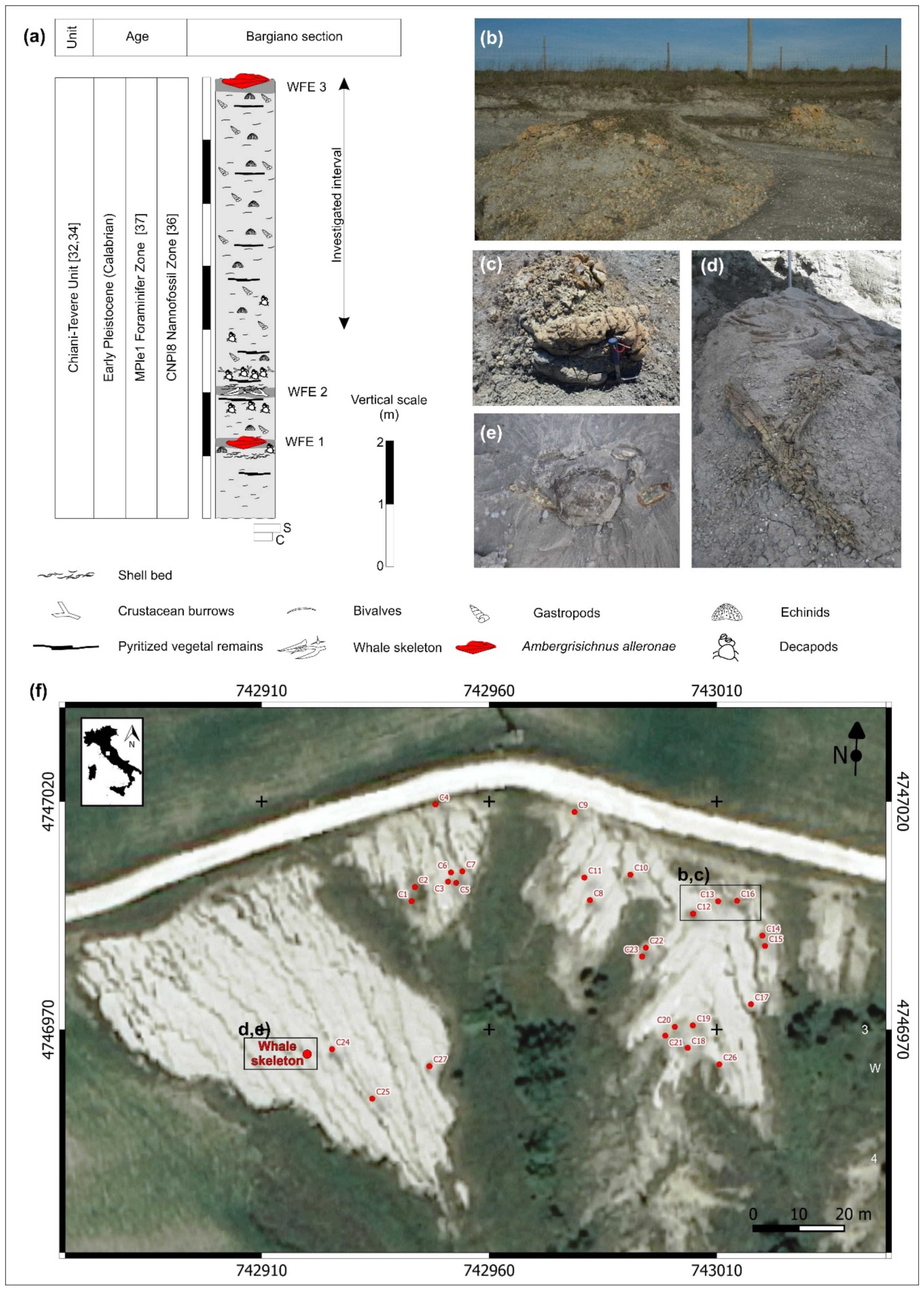
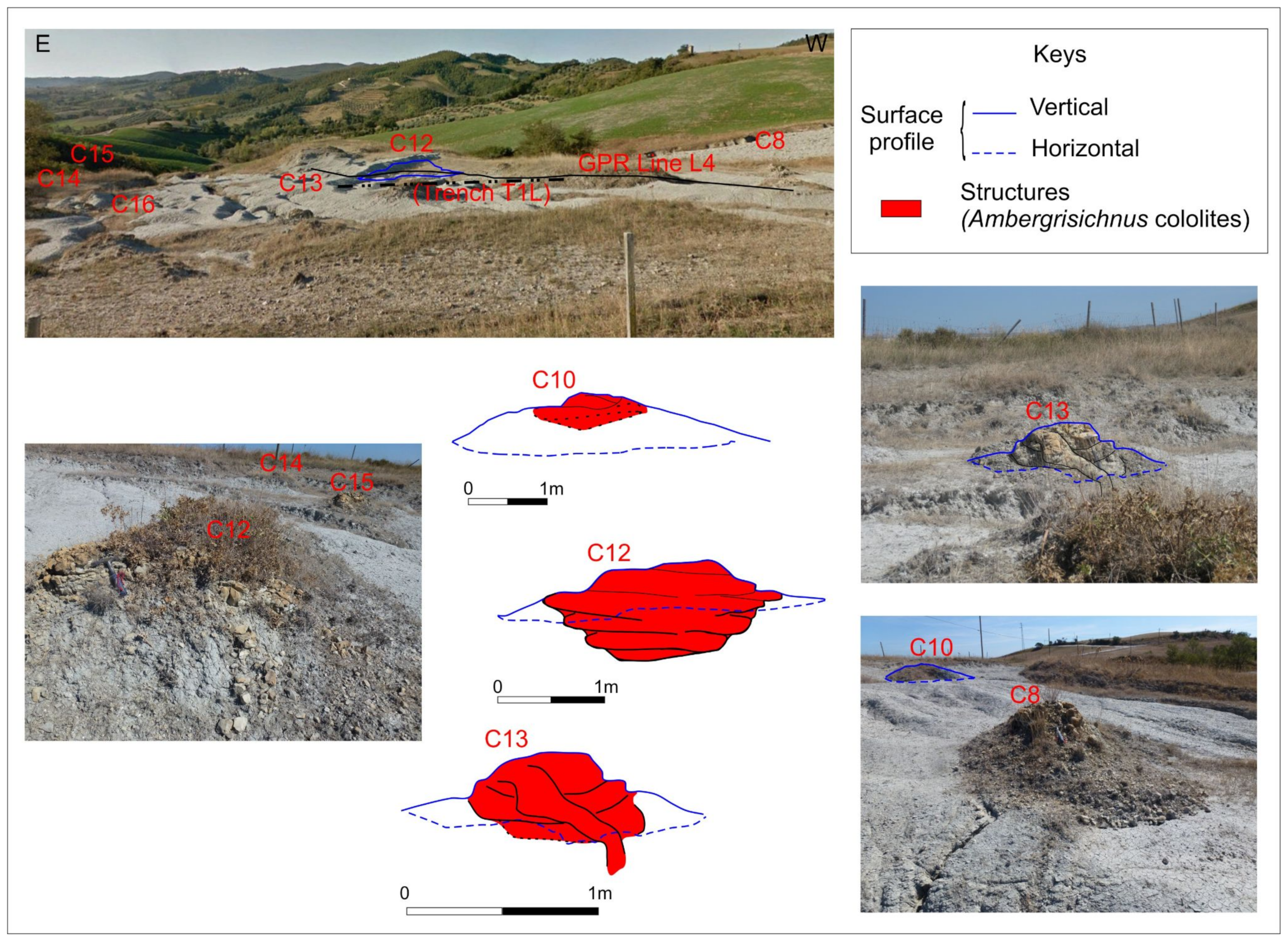
Through the years, the Bargiano site was productive from a paleontological point of view (
Figure 2). From clay sediments, bivalves, gastropods, scaphopods, echinoids, decapod crustaceans, fish remains, and shark teeth were commonly reported, along with cetacean remains or cetacean-related ichnofossils. Three Whale-Fall Events were recognized (WFE 1–3,
Figure 2a,d), with their accompanying peculiar macro- and micro-fauna (decapods, mollusks, and foraminifers, [
30,
41];
Figure 2e). As one event is associated with the presence of a baleen-whale skeleton, the other two are related to a sperm-whale and
Ambergrisichnus cololites [
30]. The larger ones are hummocky-like structures of variable dimensions, with a biconvex shape only partly protruding from the embedding clay (
Figure 2b,c), reported as complex cololites in the ichnological description [
29]. Characteristic diagnostic features of the ichnotaxon, such as striae, bulges, and concentric pattern, are often recognizable only on isolated, relatively smaller structures, or as disarticulated portions of complex structures (simple cololites: [
29]). Less frequent, almost straight cylindrical structures connect close, larger cololites below the surface. Mineralogical analyses of cololites showed a prevailing dolomitic composition (72 to 81 wt.%, [
29]), with subordinated quartz and phyllosilicates, and traces of calcite and plagioclases.
2. Methods and Field Data Acquisition
Ground Penetrating Radar (GPR) is a geophysical technique typically used for high-resolution prospecting at a shallow depth [
4]. A GPR system normally operates at a frequency range between 10 MHz and 1 GHz for geologic applications. A GPR record is based on the recording of two-way (TWT) travel-time electromagnetic pulses reflected by buried targets. These pulses are generated and recorded by transmitting (Tx) and receiving (Rx) antennae, respectively.
GPR reflections are convolved in GPR traces, which are displayed within GPR profiles, also called “radargrams”, showing trace number (or distance) vs. samples. The samples correspond to a specific TWT value, of which knowing the medium velocity can be converted to depth. After the application of a customized processing flow, the GPR data are able to provide a reliable representation of the shallow subsurface, averagely within ~10 m depth in good dielectrics. The geological interpretation process is pursued by correlating and interpreting radar reflections with outcropping formations at the surface or, when available, with direct data obtained from pits or trenches. The Em waves propagation and attenuation are governed by electrical properties of the surveyed materials, particularly the relative dielectric permittivity 𝜀
r in low loss media [
42,
43], which is linked to velocity by the formula:
where ε
r is the relative permittivity and 𝑐
0 is the velocity of Em waves in free space (~3 × 10
8 m/s). The permittivity of a material is a measure of the extent to which the charge distribution within the material is polarized in an external electric field, and it is better described by complex quantity ε
*, with the real and imaginary components representing the ‘instantaneous’ energy storage–release mechanism and the energy dissipation, respectively [
4]:
In Equation (2), the
(imaginary number) and ε″ = σ/ωε
0 describes the losses [
42] principally caused by ionic conduction, where σ = DC conductivity, ω is the angular frequency, and ε
0 is the electric constant 8.85 × 10
−12 F/m [
15,
44,
45]. Considering the operative frequency range typically used with a GPR, ε″ is often small compared to ε′ and many soils are not affected by the dispersion [
46]. A considerable increment of the measured permittivity in a porous material (e.g., sandy soils) is due to the presence of water (ε
r ~ 80), whose polar molecules are permanently polarized and oriented with the applied field [
42]. The conductivity component can usually be considered frequency independent, only related to ionic conductivity (internal fluids) or to surface charge conductivity (related to clay minerals) [
4]. Therefore, the increase of surface conductivity is often crucial as it affects the investigation depth [
47]. In lossy media, variable EM attenuation is observed, in the worst cases up to the loss of the majority of the Em energy as heat [
4].
As a consequence, the investigation depth reached by a GPR prospecting can change from 5 to 30 m in sandy units or in mixed soils with high sandy percentages [
48,
49], to less than 1 m (or even to no more than 0.25 m) with a minimal presence of humid clays [
49,
50] or in sodic terrains [
3].
The Bargiano site is characterized by clayey formation, extensively cropping out, and by a very irregular topography due to gully erosion that hampered the acquisition of a regular 2D or 3D grid of GPR profiles and also limited the antenna-ground coupling. We carried out a GPR survey at the Bargiano site (
Figure 1) using a Zond 12e Advanced GPR system (Riga, Latvia,
www.Radsys.lv, accessed on: 8 September 2021) equipped with two different antennas of 300 and 500 MHz of center frequencies, which we considered in this case the best trade-off for portability and resolution. The centimeter accuracy of GPR trace positioning was ensured by the integrated use of a survey wheel and a Global Navigation Satellite System (GNSS) receiver. The latter device is a Topcon GR-5 (Tokyo, Japan,
https://www.topconpositioning.com, accessed on: 8 September 2021) providing coordinates and elevation data through a differential correction operated in a Network Real Time Kinematic (NRTK) configuration [
51]. In addition, gullies, obstacles, and targets of interest visible at the surface were constantly annotated and mapped during the acquisition. Our entire single-fold dataset was collected using a Common Offset (CO) configuration [
52].
Table 1 reports the main acquisition parameters used during the collection of the dataset (location in
Figure 3).
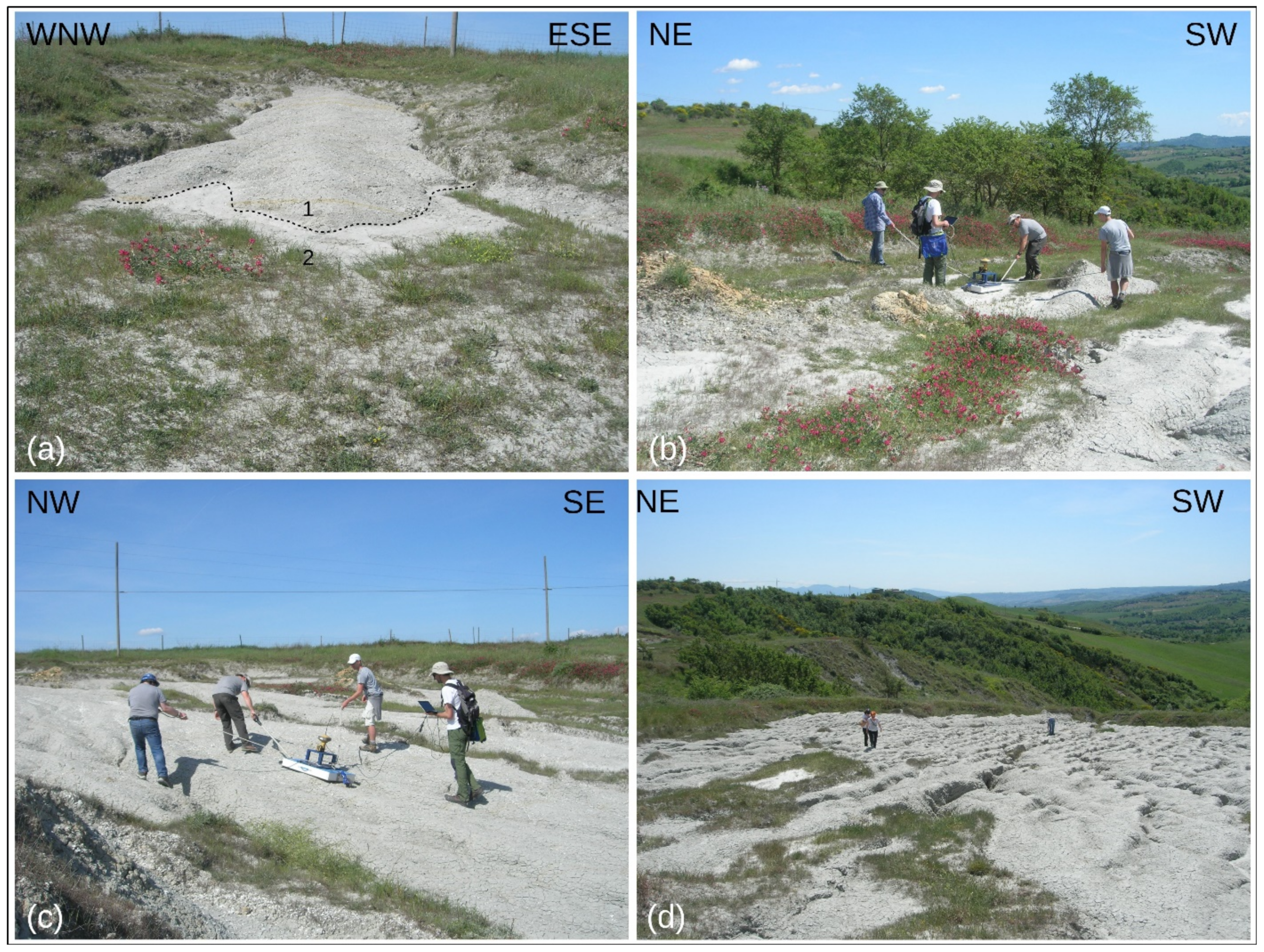
The first part of the survey was dedicated to the acquisition of some test profiles, by crossing different areas with exposed stratified clayey beds (compact, with cracks at the surface) or a cover of alternating vegetation as well as fine deposits generated by the erosion and accumulation on topographic lows. The aim was to quickly look on site at the electromagnetic response across different materials and to set up optimized acquisition parameters once the investigation depth and resolution achievable onsite were evaluated.
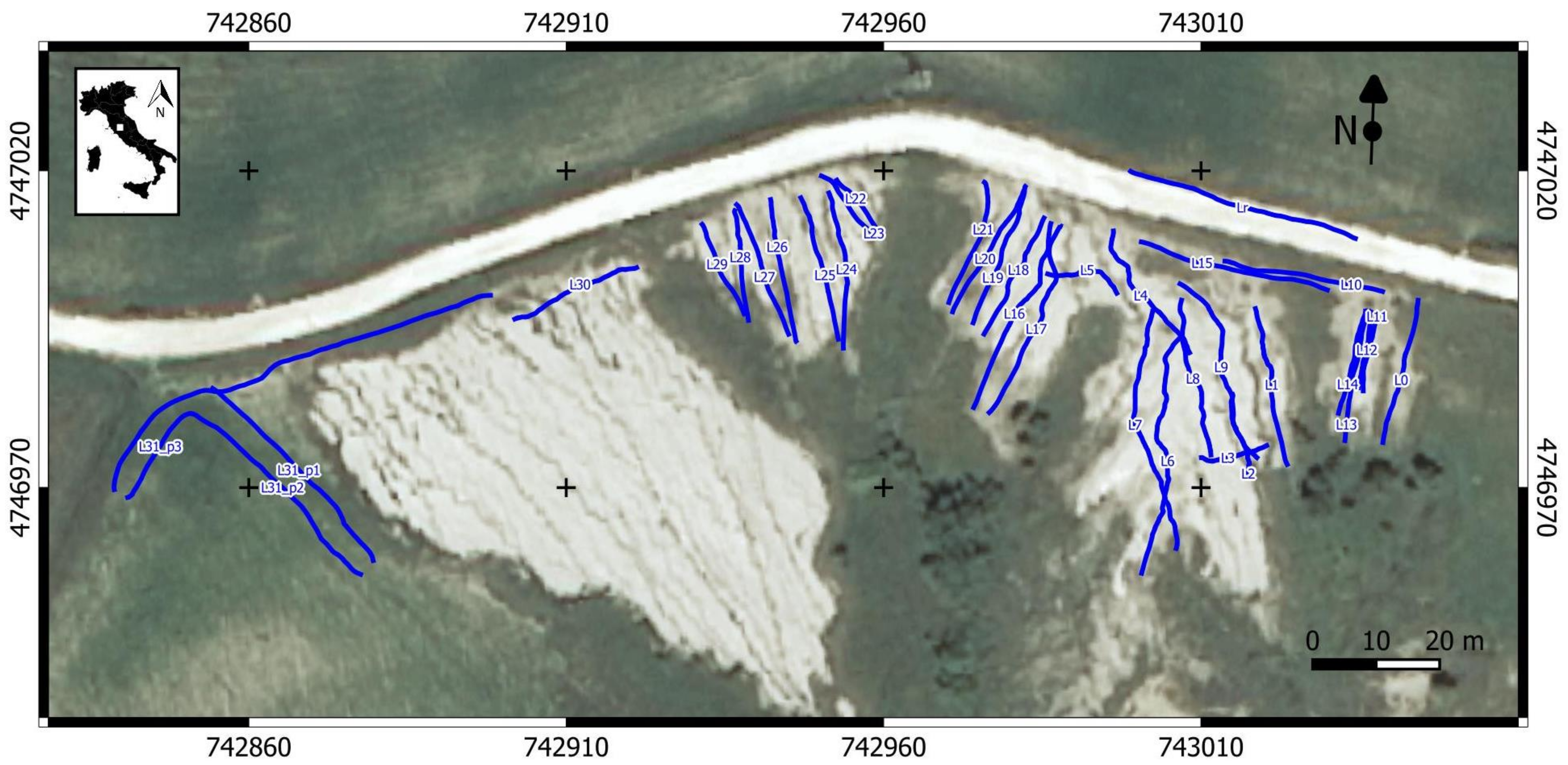
Then we recorded 33 GPR profiles mainly spreading in the central and easternmost sectors (
Figure 3 and
Figure 4a–c), whilst a zone characterized by a high density of deep channels (central-western sector, in
Figure 4d) was immediately discarded due to the high density and depth of the channels hampering GPR data collection. The rugged topographic surface prevented us from recording 2D GPR profiles using straight GPR profiles as part of a regularly spaced survey grid. For this reason, the antenna was pulled along crooked lines, where the surface was flatter and more regular, to maintain an optimal antenna/ground coupling and avoid crossing the gullies, thus reducing signal reverberations in the air. In a few cases, we passed very closely or directly across the outcropping cololites (
Figure 2,
Figure 3,
Figure 4 and
Figure 5) that were mapped and accurately measured on site during former fieldworks and successively in the laboratory [
29].
The results of GPR investigation were integrated with GPR Finite-Difference Time Domain numerical simulations (FDTD) [
53], with the aim of highlighting the cololites and fossiliferous beds buried in a relatively homogeneous clayey formation. Synthetic GPR data can provide important information during the survey planning as well as for an advanced GPR interpretation. By returning the presence and timing of complex reflection patterns, simulation aids the interpretation of subtle information embedded in field experimental data, for example to infer the electrical properties of materials, determining the geometry of reflection patterns, and distinguishing the primary reflections from multiples. Several GPR numerical modelling methods are currently available for various GPR applications [
3,
4,
54]. The Finite-difference time-domain (FDTD) method of approximation is based on Maxwell’s equations describing the behavior and effect of electromagnetism [
53,
55,
56,
57,
58]. Among the most-used commercial and open-source GPR modelling software there are Reflex-Win [
59], gprMax [
60,
61,
62], and matGPR [
63]. All these programs allow for modelling the effects of electromagnetism on a target or material, by dividing both space and time into discrete segments.
Thus, a simulation of the GPR wave propagation through subsurface materials was obtained, with boundaries and geometry of objects (i.e., representing geological structures) that are segmented into cubic cells [
64] (“
Yee cell”) to create the computational domain. These cells are relatively small in comparison to the GPR wavelength, but a staircase approximation was used to model curved boundaries. The electric fields and magnetic fields are located on the edges and on the faces of the cells, respectively. During the modelling process, different values of physical properties were assigned to each modeled object: Typically, the relative dielectric permittivity ε
r is varied as well as the conductivity σ, whilst the magnetic permeability µ is generally a unity. Thus, after the discretization of the whole area into Δx, Δy, and Δz segments, and once we defined the above-mentioned electrical properties in a mesh grid, the FDTD computation proceeded with a substitution of partial derivatives by differential quotients in Maxwell’s equations. Using the GPR response obtained by the modelling as well as by experimental profiles, we aimed to identify a characteristic GPR signature to (1) drive the operators to a pre-survey choice of optimal antennae and acquisition parameters, (2) understand what kind of GPR signature to expect within field data, thus supporting GPR interpretation across sectors without any outcrops, and (3) provide a reference GPR record for future paleontological works in such environments. Following the generation of synthetic data, we carried out a GPR attribute analysis to better inspect our data and extract additional information constraining the GPR interpretation. The attribute analysis is a relatively cheap and fast tool, commonly used for the interpretation of reflection seismic data [
65,
66,
67], which aids in emphasizing the subsurface geophysical features in complex geological sites. Like in the reflections seismic technique, a single GPR attribute or a multi-attribute integration can provide details on the subsurface physical or geometrical properties of the media. GPR attribute analysis is still not very widely used, but in recent years, it has been surely growing for different applications, such as fault and fracture characterization [
7,
10,
68,
69], archaeological studies [
23,
70], as well as in sedimentological and glaciological applications [
71,
72,
73].
GPR modelling as well as attribute analysis might represent innovative tools to improve the detection and characterization of fossiliferous layers. According to our knowledge, such techniques were very rarely used in paleontological studies [
74], and we speculate that our attempt may represent the first combined application in this field. Among the multitude of seismic attributes available, we selected and computed the instantaneous amplitude and phase, which were pioneered for the detection of the “bright spots’” [
66] in reflection seismic. The instantaneous attributes, which are based on complex trace analysis, are computed through the Hilbert transform for each sample of the seismic or GPR trace. Thus, given:
where
u(
t) is the trace,
i is a complex number, and
y(
t) is the quadrature obtained from the Hilbert transform [
7]. The instantaneous amplitude and phase are obtained from:
With these attributes, we aim to enhance high reflective bodies and signal discontinuities. The first are emphasized by the instantaneous amplitude (i.e., sensitive to the amplitude), which is related to acoustic impedance or dielectric contrasts in seismic and GPR techniques, respectively. It is independent of phase and it is often called “Reflection strength”, whose gradual lateral changes can be produced by the interference of reflections arising by lateral variations of bed thicknesses [
66]. In reflection seismic, sharp local changes may help to discriminate bright spots and possible gas accumulation. Commonly with GPR, stratigraphic boundaries, changes in the depositional environment, thin beds (tuning effects), and faulting can be highlighted, thus providing spatial correlation to lithologic variations and presence of structural discontinuities. These features are better enhanced using the instantaneous phase (i.e., sensitive to the phase), being linked to the propagation phase of the wavefronts [
7]. The phase is independent of reflection strength and the display is obtained by assigning the same color to each peak, trough, or zero-crossing of the real trace, thus allowing to follow the phase angle trace-to-trace. Weak but coherent events become clearer using the instantaneous phase, thus emphasizing the continuity (and so also the discontinuity) of reflected events [
66], which might be interpreted as faults, pinchouts, angularities, and variations of dip patterns. In this study, we propose the combined use of the instantaneous amplitude and instantaneous phase, which are physically independent and thus they may provide complementary information for detection and characterization of fossils.
2.1. GPR Finite-Difference Time-Domain Numerical Simulations (FDTD)
We created different models using Reflex-Win [
59] software (v. 9.1.3) to simulate the presence of fossils within a clay medium, thus generating synthetic GPR profiles to reproduce the complex field conditions of the study site. The FDTD was used prior to the acquisition to achieve information about the vertical resolution and investigation depth achievable in a conductive medium using 300 and 500 MHz operative frequencies (modelling parameters in
Table 2) and, thus, to arrange the survey on the field. Due to the absence of any preliminary geophysical data or dielectric measurements at the study site (
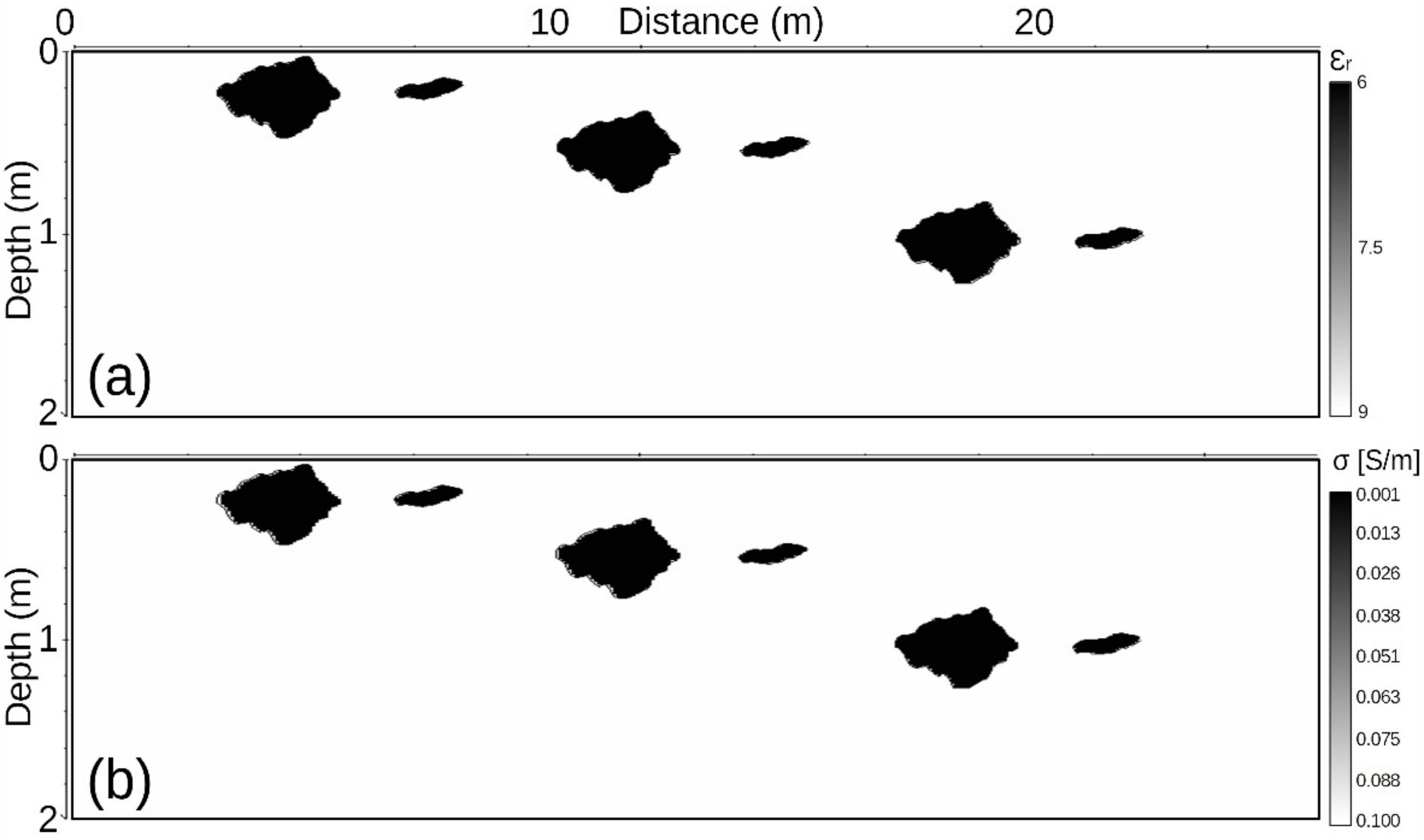
Figure 5), under some assumptions (flat topography, constant physical parameters, etc.), we have initially created a simple model (
Figure 6), thus simulating three cololites and relatively small fossil beds located at increasing depths (~0.20, 0.50, 1.0 m). We decided to use average physical parameters (dielectric permittivity ε
r and, electrical conductivity σ) for the surveyed clays and dolomite obtained from literature [
3,
4], thereby assuming a non-magnetic medium (μ
r = 1) (detail of parameters in
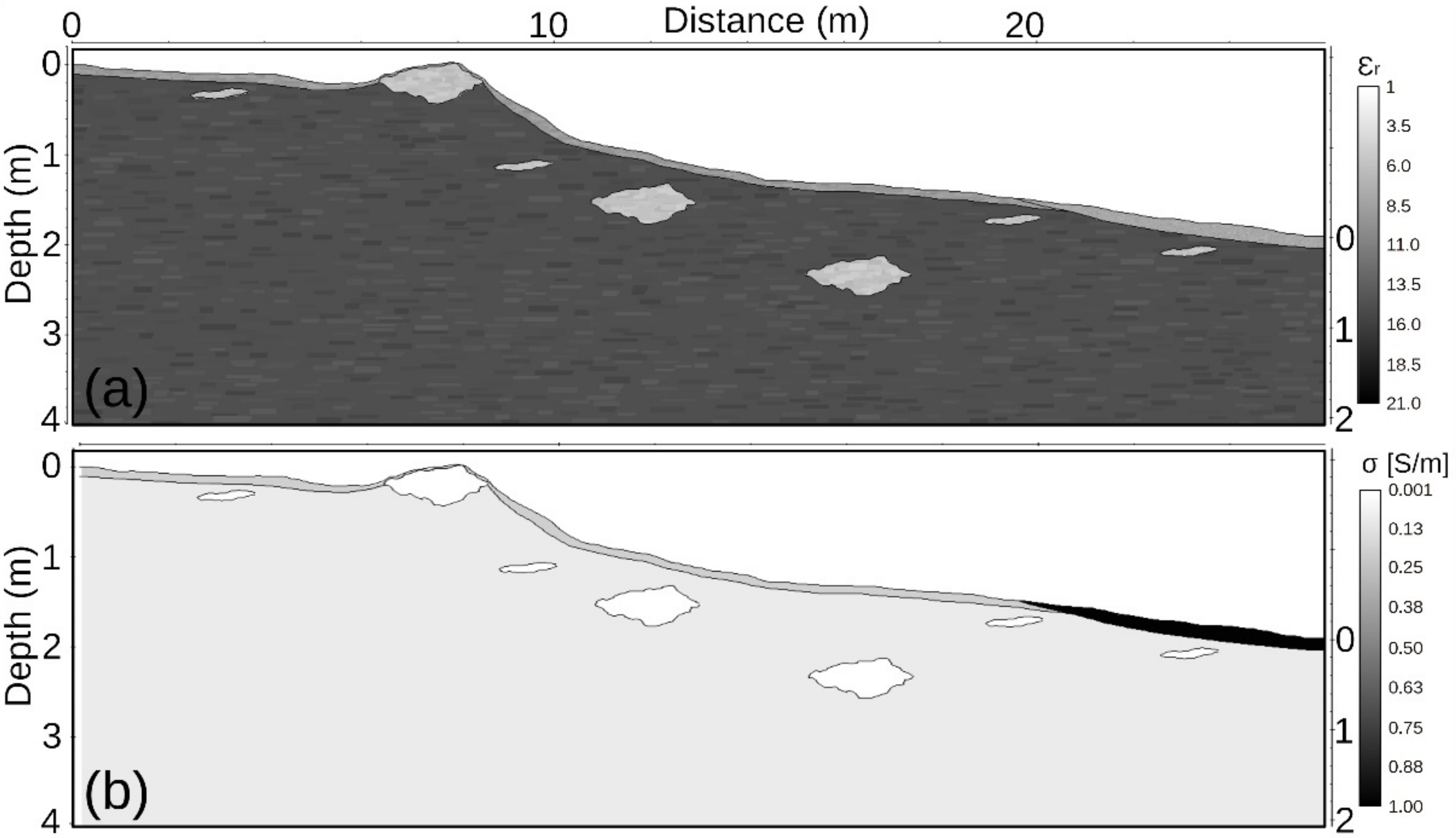
Table 3). To improve the reliability of our synthetic data, with the same purpose, we have successively produced a more complex and realistic model (
Figure 7) by simulating environmental complexities characterizing the study site (detail of parameters in
Table 4), also using the observations achieved during preliminary surveys. The preliminary fieldwork suggested a lower velocity of media in depth and a higher conductivity of shallower deposits, which produces severe GPR signal attenuation in some areas. Thus, the cololites are centered at depths of ~ 0.20, 0.50, and 1.0 m from the topographic surface and the fossils beds lay at ~0.2, 0.3, and 0.6, both located in key points in relation to the embedding media. In comparison to the first basic model, we considerably increased the average conductivity values of materials and introduced new layers with disturbances (i.e., statistical variations of the dielectric permittivity) to ensure the model displays heterogeneities; in addition, we added a realistic topographic surface, which was later refined by extracting elevation values from the GNSS recordings of experimental profile L1. The new simulated layers include a shallow ~10 cm thin polygon representing altered clays to reproduce the presence of a finer dry soil and mud cracks visible at the surface, and another polygon simulating a thicker (up to ~20 cm) altered unconsolidated clay-loamy deposit, typically observed laying at the base of the slope. For these two layers, we chose a finer texture, refining the parameters introduced for the statistical fluctuations, to simulate high conductive deposits faithful to a severe real scenario (
Table 3). White random noise (1%) with a nominal frequency of 300 and 500 MHz, respectively, was also added to raw synthetic profiles to make them closer to experimental data. Using a Dell Workstation with Intel(R) Core(TM) i7-4712HQ CPU @ 2.30 GHz and 16 Gb RAM and the reported parameters, the simulations took a time range for each profile spanning from a few seconds to a couple of minutes for the more complex models (e.g., model 2 with frequency source of 500 MHz).
To summarize, we decided to increase the permittivity of deposits in depth assuming a higher content of humidity within the clays (εr = 15), whilst a lower permittivity value (εr = 8–9) was assumed for the shallower clayey layers, due to lower compaction and higher relative presence of air. The conductivity σ was assumed to be higher (up to 1 S/m) at a shallower depth due to the alteration of clayey deposits producing the total attenuation of the radar signal observed during the GPR fieldwork.
2.2. GPR Data Processing and Computation of GPR Attributes
The GPR data processing is typically based on techniques borrowed and adapted from reflection seismic surveys [
75], well summarized by [
4]. We processed the experimental and synthetic GPR profiles using the software Prism v. 2.60 (
http://www.radsys.lv/en/index/: [
76], accessed on: 8 September 2021) and Reflex-Win v. 9.1.3 [
59], respectively, in order to improve the S/N ratio, obtain reliable target geometries, as well as to increase the data interpretability (processing parameters are summarized in
Table 5). The synthetic data obtained from the second model required the application of a basic processing flow, including amplitude recovery (correcting for energy losses), bandpass Butterworth filtering (100–400 MHz and 300–700 MHz, respectively), f-k migration, and a topographic correction. A time-to-depth conversion was finally applied using GNSS elevation of profile L1 and a V
em = 0.075 m/ns. On the experimental data, editing and quality control were performed first, by checking and fixing issues on GPR traces, GNSS coordinates, and elevation values. After several tests, we refined a processing flow (details in
Table 3) including amplitude recovery, flattening of first arrivals, and time-zero correction; following a spectral analysis, customized filters were applied to remove low- and high-frequency components and to attenuate horizontal bands locally generated by high conductivity of media and scarce antenna-ground coupling. A velocity analysis accomplished through the fitting of hyperbolic diffractions allowed us to estimate an average velocity value of 0.075 m/ns, in agreement with literature ranges available for clays [
4]. Such a velocity value was used for the f-k time-migration as well as for the topography (static) correction and the time-to-depth conversion. The processed profiles highlight several radar reflections suggesting the presence of a subsurface structure within a max depth no greater than 1.5 m. These reflections have been successively enhanced by the computation of GPR attributes, specifically the Envelope and Cosine Phases [
7,
10], which improve the display of subsurface reflectivity and provide details on the geometries of buried geological structures. In the following paragraph, we show the results of our synthetic modelling and the most representative experimental GPR profiles, including the attributes, with examples for both 300 and 500 MHz data. In the final discussion, we also provide a punctual validation of our interpretation using four trenches, excavated along the tracks of selected GPR profiles, which displayed promising subsurface reflections.
3. Results
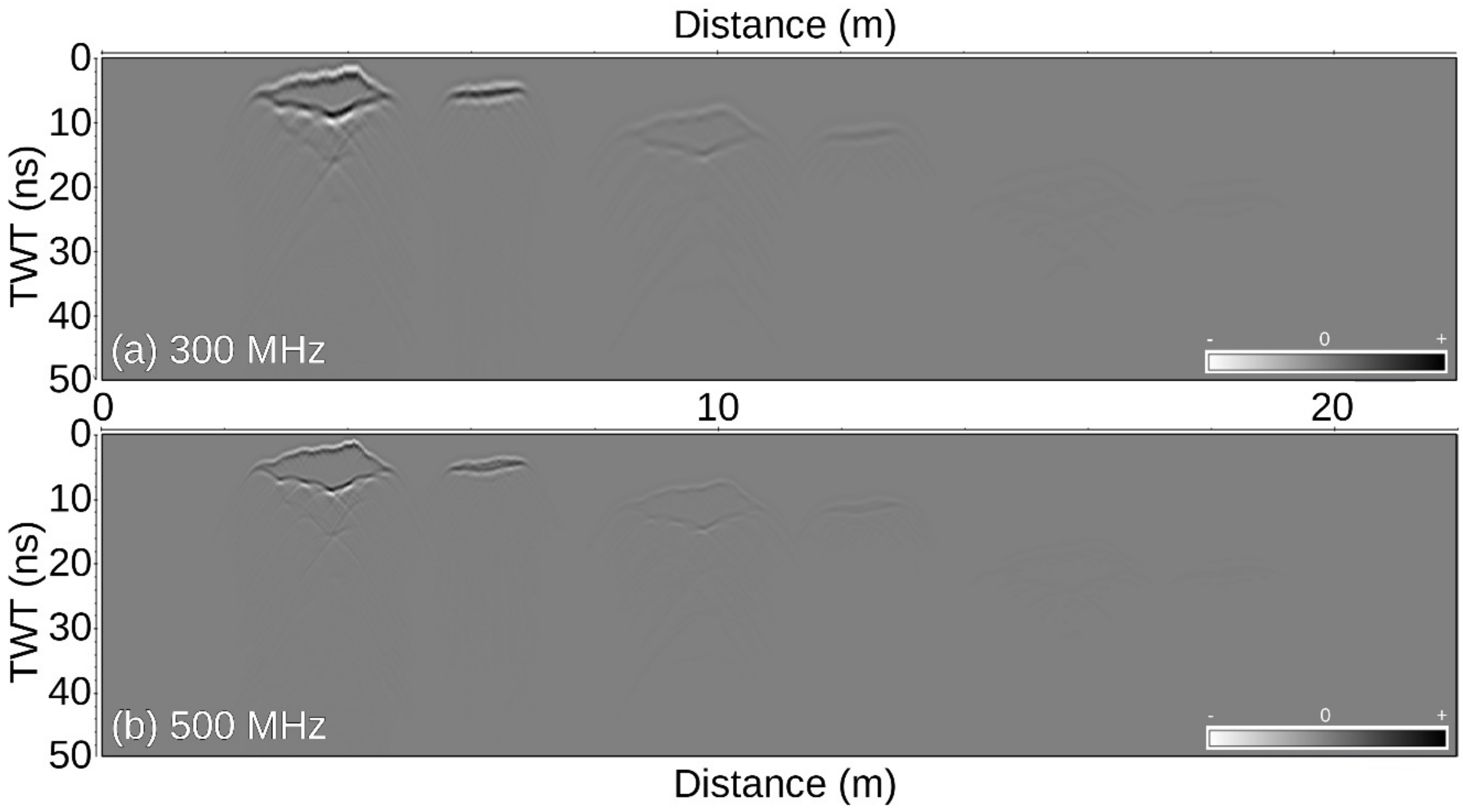
Figure 8 displays the results of a simulation obtained from model 1 of
Figure 6. Six complex reflections are located within a TWT of ~25 ns, three of them related to simulated cololites whilst the other three represent fossiliferous beds. One can easily notice the higher resolutive capability of the 500 MHz synthetic data in comparison to the 300 MHz, aiding in better distinguishing the details and geometry of the buried targets. We estimate that the vertical resolution (λ/4) for 300 and 500 MHz frequencies is ~0.08 and 0.05 m, respectively. The simulated cololites show both top and bottom reflections on raw synthetic data, whilst for the fossiliferous beds (~0.1 m thick), only the 500 MHz synthetics clearly resolve the top and bottom reflected arrivals. The interference between several hyperbolic diffractions and reflected signals creates complex simulated reflection geometry particularly on the lateral sides and bottom sides of the targets, where complex “bow-tie” arrivals are also visible [
3,
75]. Assuming a V
em = 0.075 m/ns for the clay formation, the deeper reflections are included in an estimated depth range no greater than ~1.50 m. Thus, the detectability of the deeper target is more difficult due to the high attenuation of radar signal: At a depth of ~1 m, the reflections are already very weak, particularly for the 500 MHz data, suggesting not to push the interpretation to greater depths. To summarize, the FDTD results provided by the first basic model highlight a possible maximum investigation depth no greater than 1.5 m, and also suggest that combined use of both antennae may provide complementary information to resolve and detect fossil layers of variable sizes at variable depth. Following the reproduction of reliable fossil geometries, our simulations also provided a possible characteristic signature of fossiliferous layers to be searched in the experimental data. Thus, following the results achieved from the first model, we show other synthetic profiles from a second model (
Figure 7). These synthetic profiles are illustrated in
Figure 9: The raw synthetic profiles for the two frequencies used are displayed in
Figure 9a,c, whilst the processed version is reported in
Figure 9b,d. The reflections generated by fossil structures close to the topographic surface display high to moderate amplitudes at progressively greater depths, due to signal attenuation operated by high conductivity of shallow simulated deposits.
The strong attenuation causes very weak or no reflected signals at a greater depth (already at ~1 m) in both 300 and 500 MHz synthetic profiles, with random noise also partially masking the reflections. In particular, total attenuation is visible on the right side of the synthetic profiles: It should be noted that the fossiliferous bed at a shallow depth (~20 m distance) is visible only on its left half portion. This consideration suggests that every kind of target located beneath such a high-conductive layer at shallow surface will be essentially not detectable.
Due to the amount of GPR data recorded in the field, only the GPR profiles showing the most peculiar GPR signatures and interesting reflected events are reported in this paper. The quality of a few of the 300 MHz profiles was operatively affected by the bigger size of the antenna during the fieldwork: Particularly when crossing areas characterized by rugged topography or across very irregular cololites, the antenna had a reduced coupling with the ground, generating localized reverberations (ringing). However, the related traces were annotated during the acquisition, in order to avoid further data misinterpretations. In other cases, chaotic, poorly continuous and not well-defined reflections were observed locally, due to the interference of reflections and hyperbolic diffractions with local pervasive sub-horizontal reflections.
In other points surveyed, we detected reflection patterns of good continuity, particularly close to the cololites outcropping on the compact clay formation, which we have analyzed computing the GPR attributes. More specifically, the first selection of GPR profiles is reported in
Figure 10, where raw and processed profiles L25 and L13 are illustrated.
The first crosses the cololite C3, whilst the second was recorded on the eastern area with no fossils outcropping at the surface.
Figure 10a,c displays a difference in reflectivity with a clear lateral variation due to strong attenuation of surveyed media, also affecting the ground wave arrival, which towards the end of both profiles is strongly attenuated. The processed profile L25 (
Figure 10b) shows high reflectivity within the first meter depth, with a rapid decrease down to 1.5 m depth along the profile distance range 22–12 m, in which reflections of poor lateral continuity are visible. However, within the distance range of 0-8 m, the signal penetration is practically absent or limited to a few tens of decimeters and characterized by weak reflections.
Only at about a 10 m distance, the GPR profile shows higher GPR penetration (down to ca. 1.5 m) and high reflectivity: Here, undulated (~0.5 m depth) to sub-horizontal reflections of limited lateral continuity (<~2 m long).
Figure 10d displays similar reflections for profile L13, characterized by reflections of moderate amplitude and poor lateral continuity within the interval 0–10 m, for a maximum investigation depth of ~1 m. Similar to L25, almost total attenuation is observable within the distance range 21–13 m.
A higher reflective body is visible only in the distance range 10–12 m, with a laterally limited (<~2 m long) sub-horizontal reflection pattern within the first meter depth; this package of reflections is slightly rotated and laterally bound uphill by sub-vertical discontinuities. Such considerations on the reflectivity and reflections geometry of GPR profiles L25 and L13 can be extended and confirmed more accurately after the computation of the GPR attributes. The instantaneous amplitude reported in
Figure 11a,b enhances the subsurface reflectivity, confirming it is limited to the first meter of depth for both profiles, and it is characterized by lateral variations. This attribute also confirms the almost total attenuation occurring from the base of the slopes to the end of both profiles, suggesting very high values of conductivity for these sectors. Here, possible buried targets, even if located at a shallow depth, are basically impossible to detect, confirming the results obtained in our synthetic example from model 2. This attribute confirms the presence of two reflective bodies within the center of both GPR profiles: One wider and deeper in profile L25 and another shallower and marked by sub-vertical amplitude discontinuities in profile L13. However, the continuity as well as the presence of lateral discontinuities of reflections can be better appreciated in the instantaneous phase attribute images (
Figure 11c,d). This attribute permits the interpretation of the stratigraphic boundaries and reflections geometries, as in profile L25 (
Figure 11c) in which an undulated continuous reflection is visible (range ~6–12 m), with the convex shape matching the high reflective body detected in the corresponding amplitude profiles. Another advantage of this attribute, as it is independent by amplitude, is the capability to extend the display of reflected events in depth, where the amplitude profiles are not interpretable due to attenuation. However, although some shallow undulated reflections are also visible in the profile of
Figure 11d, the deeper sector of this profile shows some migration artifacts (smiles). These features can be possibly generated by the poor level of signal and random noise contamination, or by a velocity variation in depth. However, given that our survey target is limited to a maximum of 1.5 m, our interpretation was focused on the shallower depth interval; here, undulated reflections, laterally variable in thickness with pinch-out closures, are visible. In particular, over the sector marked by strong attenuation, these reflections are also dissected by sub-vertical phase discontinuities with centimetric offsets.
In
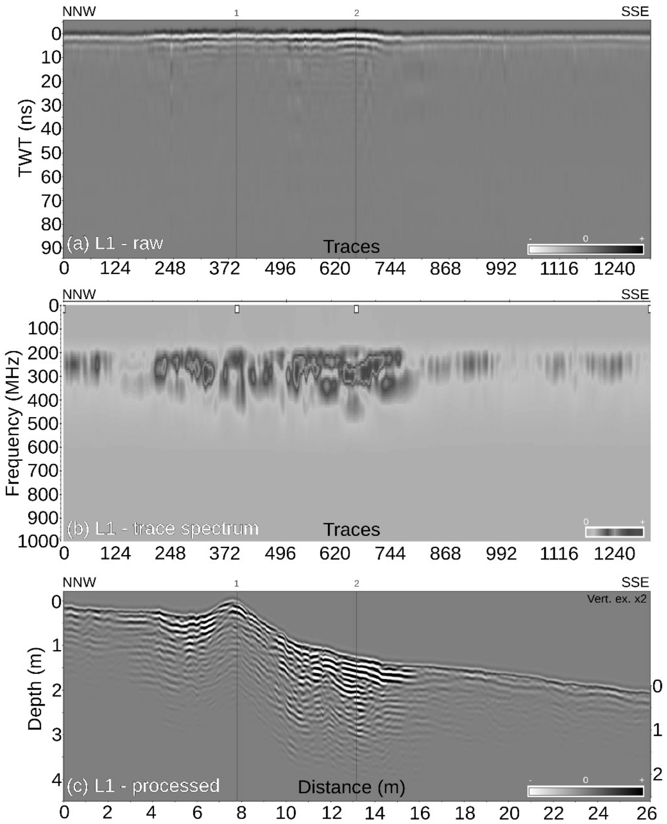
Figure 12, we report an example of a 500 MHz profile (L1), which crosses the cololite C14 outcropping just a couple of meters south-west of the cololite C15.
Figure 12a shows the raw GPR profile, which, without any amplitude recovery function applied, displays only higher reflectivity at early times, particularly in the central sector. The first vertical mark suggests the position of cololite C14, also visible due to the local topographic height at about 8 m.
With the second mark, we noted a sector in which the antenna-ground coupling was good due to outcropping clay formation, which was flat and very compact without any cover of altered deposit or grass. On the contrary, at ~16 m, a lateral decrease of reflections amplitude marks the transition to an area characterized by strong attenuation (16–26 m along the profile), similarly to previous GPR data. An amplitude trace spectrum of profile L1 is visible in
Figure 12b, displaying a bandwidth centered at about 250 MHz in the range 4–15 m along the profile, whilst the frequency content of surrounding areas is extremely poor. The corresponding lateral change in reflectivity is much more visible in the processed profile (
Figure 12c), showing the geometry and attitude of main reflections within 1.5 m depth. Interestingly, the more reflective zones surround outcropping C14, which shows, differently from the synthetic and 300 MHz data, a moderate reflection on its top portion without any reflection in the deeper sector; this behavior can be possibly due to a minor amount of energy reflected back to the antenna when crossing C14, but we noticed it is more common in the 500 MHz profiles crossing outcropping cololites.
Possible explanations can be suggested for the single or combined effects of a minor antenna-ground coupling and attenuation, caused by: (1) The irregular and steep cololite shape on its top; (2) high conductivity of cololite cover at the surface; and (3) a smoother transition to underlying clays causing a lower dielectric contrast (or/and in combination with higher conductivity) on the bottom side of the cololite itself. Looking at the area at a 12–14 m distance, a clear strong reflection is visible at a shallow depth and another one deeper at ~1 m depth, resembling the one at an intermediate depth in the synthetic profile of
Figure 9d. In
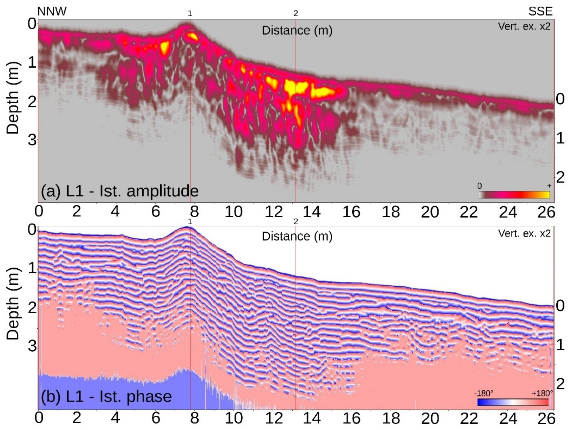
Figure 13, we analyzed the GPR profile L1 computing both instantaneous attributes.
Figure 13a illustrates the instantaneous amplitude, with a moderate-to-high reflectivity surrounding the cololite C14, which on the contrary, displays a moderate reflectivity in the first 40 cm and lower in depth, as highlighted in the conventional GPR images. High energy is visible in the central area, up to ~1.20 m depth. The GPR profile in the sector between 16–26 m displays low reflectivity and only within the first 0.30 m depth, confirming low penetration of radar signals.
Figure 13b displays the instantaneous phase, computed on the same GPR profile. In addition, in this case, it is very effective to map the geometry of reflections, independent of amplitudes, where the signal attenuation is also strong. This way, a depth extension of profile interpretability is again possible at 16–26 m distance intervals along the profile. This attribute is also very useful to emphasize the geometry of possible buried bodies, highlighting the continuity of reflections very well: It displays sub-horizontal reflections of constant thickness in the southernmost sector as well as undulated reflections with local thickening nearby the cololite.
4. Interpretation, Validation and Discussion
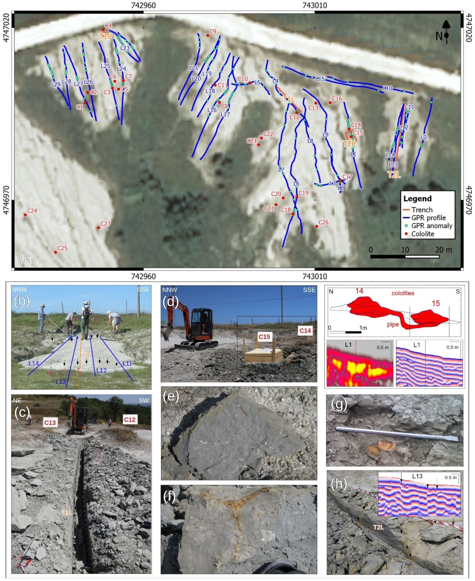
Our interpretation was accomplished for the entire dataset in order to generate a map of the GPR anomalies detected along each profile.
Figure 14 shows a mosaic image summarizing our interpretation, supported by photos of the excavation campaign. In
Figure 14a, we summarize all the GPR anomalies recognized within the processed GPR data, except the westernmost profiles Lr, L30, and L31, due to no signal penetration. In other sectors, we delimited some excavation zones combining the interpretation of conventional GPR profile reflections as well as peculiar GPR attributes signatures approximately within the first meter depth. To preserve the site as much as possible, a couple of sites were finally selected and dedicated to ground-truth the GPR reflections (e.g., site in
Figure 14b). Thus, to avoid damaging outcropping cololites, which are highly unstable as they are permanently exposed to weathering and soil erosion, we opted to use manual excavation tools and a small narrow shovel excavator (
Figure 14c,d). This choice limited the overall excavation depth averagely to within a 0.5 m depth, as deeper trenching would have required bigger mechanical excavators.
We excavated two linear trenches (T1L and T2L, location in
Figure 14a): T2L was excavated in the easternmost area along profile L13 (~20 m long, ~50 cm deep), where no fossils were visible at the surface (
Figure 14b). The T1L was located close to a sector of profile L4 (~10 m long and 30–40 cm deep) and ended up close to cololite C12 (
Figure 14c). Regarding where the other two excavations (position in
Figure 14a) were located, one was close to cololite C4 (T1P) in an area uphill of GPR profiles L25 and L23 (
Table 2), where some fragments of fossils were found at the surface, and the second (T2P) in between cololites C14 and C15 (along the track of lines L1,
Figure 14d). T1P and T2P cover an overall surface of ~3.5 m
2, reaching depths of ~50 cm and ~1.5 m, respectively. All excavations show a shallow (a few centimeters up to ~10 cm thick) dry and altered clay layer, laying above humid, dark, massive, and very stiff clay beds (
Figure 14c,g,h). This bottom layer hindered the mechanical operations of excavation, preventing the operator from reaching deeper levels. This mechanical behavior can be attributed both to the progressive compaction of the clays with increasing depth, and to the partial dissolution of shells and the circulation of fluids enriched in CaCO
3. Locally, the trenches show clays with spotted shell-enriched layers, shell lags, as well as bioturbated layers, becoming particularly hard and compact (
Figure 14e–g). Their sparse distribution typically hinders both hand-made and mechanical excavation operations, but the GPR profiles aided us to identify areas encompassing fossil layers within surrounding clays maintaining a massive appearance and the dark-grey color (
Figure 14e,f). In more detail, the ground-truthing operated close to the three analyzed profiles provides results and details revealing the nature of reflections correlated with buried stratigraphic and structural geological features (
Figure 14d,h). The excavation of trench T1L, decided once some hyperbolic diffractions were detected in the central sector of profile L4 (depth < 1 m), does not provide any evidence of fossil layers to correlate with the GPR signature. However, a combination of discontinuous layers of compact clays, enriched in shell fragments, and a set of vertical joints (
Figure 14c) are found lying above a hardened, dark clay layer at ~50 cm over a surface of >1m
2. The excavation was stopped before finding the lateral boundaries of this layer, as the operations proceeded too slowly (30 cm depth reached in over half an hour), and also to avoid damaging the outcropping cololites (C12-C13,
Figure 14c). The trench T2L does not show any buried continuous fossil layer or cololite within the 50 cm depth range, but we could find only spotted occurrences of layers locally enriched in mollusk specimens or bioturbation (
Figure 14e,f). This result confirms the observation that, although macrofossils are widespread across the study area, they tend to gather in well-defined layers particularly near bones [
30] (
Figure 14g) or cololites [
28,
29]. Both linear trenches T1L and T2L head off several sub-vertical fractures, striking between N305 and N330, which are easily recognizable by the presence of a thin brown hardened crust also at the surface (
Figure 14b, black arrows). Nonetheless, the processed GPR profile shows a reflective package and high reflectivity as well as clear phase discontinuities enhanced by GPR attributes (inset of
Figure 14h), explainable by a combination of stiff clay blocks bounded by steep fractures (
Figure 14h, black arrows). The most interesting link between GPR reflections as well as the instantaneous attributes signature with field structures is visible from the excavation done close to structures C14-C15. The trench (~1.5 m deep) was carried out according to an approximately square perimeter around the cololite C15. The operations were then completed with the insertion of a semi-rigid metal plate under C15, necessary to detach this fossil structure from the underlying clay deposits. However, such operations revealed an irregular shape of C15 at its base, suggesting that the size of this structure was bigger and deeper than expected from surface observations. In addition, we found a buried connection between emerging mounds C14 and C15~1 m long and ~20 cm in diameter with a quasi-tubular shape, which explains the high reflectivity and geometries also highlighted by GPR attributes (cololites scheme and attributes excerpt on the right side of
Figure 14d). Thus, cololite C15 was extracted (
Figure 14d) and recovered for musealization, and it is currently exhibited at the Allerona Museum.
Using field observations, trenching results, and geotechnical data available for the study area, we can thus infer a qualitative explanation for the overall moderate-to-low investigation depth and quality of the experimental dataset. As known, the presence of clay deposits is frequently not an ideal condition for a GPR investigation [
4], and even worse for highly compact beds or free water [
77,
78]. The various amounts of clay minerals, clay mineralogy, and the presence of cations from other sources (i.e., feldspar fragments, organic matter) reflect a high variable size, surface, cation exchange capacity (CEC), and capability to retain water of clay minerals, affecting the electrical properties ([
4,
77] and references therein). Differences in CEC, associated with the variation of the electrical conductivity, usually reflect different clay mineralogy, with e.g., kaolinite or illites showing values significantly lower than smectites or vermiculites [
4]. Thus, soils with a higher content of smectites or vermiculites (higher CEC) cause higher attenuation than soils with equivalent percentages of kaolinite or illites (lower CEC values) [
4,
78].
Geotechnical laboratory analysis of undisturbed samples of clays [
40] suggest a composition dominated by kaolinite and illite (
Figure S1). Such data allowed us to classify deposits in the range of “low plasticity clay”, so the presence of high plasticity clay such as montmorillonite or smectite, as well as high presence of organic matter, can be excluded. Preliminary results from mineralogical analysis of clay samples between Allerona quarries and the study site confirmed these results [
40], which are also in agreement with literature data in the region [
39]. In the latter case, the presence of kaolinite and illite in mixed clay phases was clearly highlighted, as well as the total lack of high plasticity clay, confirming that such a composition can be assumed for the clay fraction at Bargiano. Following such considerations, the clay composition, with prevailing kaolinite and illite (plus an average content of 15% CaCO
3, [
39,
40],
Table S1), ensured sufficient dielectric conditions for a successful GPR survey in a maximum, but variable, depth range of 0.5–1.5 m. This threshold represents the bottom transition to more compact clays with higher water content, and it is marked by instantaneous phase attribute, showing an undulated reflection with good continuity in the above GPR profiles. However, even if the experimental conditions for a GPR survey found in this study remain critical in humid clays, it is worth noting that the loss of GPR signal was almost complete in areas covered by a shallow layer of dry, fine, and unconsolidated clayey deposits (
Figure 14a,b, e.g., at the end of profile L13). These deposits are clearly produced by weathering, followed by re-deposition of the resulting material in the most topographically depressed zones, such as at the base of the outcropping cololites as well as downhill of areas with high slope gradients. In such areas, the field scenario is well matched with GPR simulations, which already highlighted very scarce or null targets detectable beneath high-conductive surface media. Although resistivity measurements would certainly help to better constrain the used literature values, thus improving the reliability of software-based models, in absence of dedicated laboratory analysis, we speculate the high conductivity of finer deposits caused by a selective accumulation and enrichment of conductive minerals. Such fine deposits reduce the GPR penetration so strongly, already at a shallow depth (e.g., ground wave), that the detection and interpretation of buried structures’ reflectivity are hampered in both conventional and amplitude-based attributes profiles. On the other hand, it is worth noticing the greater amount of information recovered by the instantaneous phase attribute, which independently of amplitudes, extend the interpretability of structures’ geometry in depth, providing more details of stratigraphic geometries and boundaries (e.g.,
Figure 11d,
Figure 13b, and
Figure 14d with right-side inset,h).
From the operative point of view, the complex topographic surface characterized by steep areas and high density of grooves forced us to pull the GPR antenna along crooked tracks instead of using a regularly spaced grid of straight lines. Thus, during the survey, we took particular care to maintain a slow antenna-pulling velocity, dodging the grooves to ensure high coupling. In the cases in which it was impossible to drive the GPR antenna without crossing grooves, we used GPR marks and we took accurate notes of GPR sectors characterized by amplitude-saturated spikes and reverberations. With this solution, post-processing trace killing/despiking strategies can be used during the data processing, and a simple interpretation of disturbed traces can also be considered. However, it is worth noting that the use of a single antenna for a bidimensional survey was a pro due to its limited size and maneuverability, whilst a 3D survey e.g., with multi-array antennae, would not be possible in such field conditions.
To summarize, our GPR study shows we can identify the presence of cololites or parts of them overall looking at moderate to high amplitude reflections in conventional GPR profiles (
Figure 10b and
Figure 12c), with geometries resembling the ones highlighted by simulations (
Figure 9b,d). The study show it is possible to identify with sufficient certainty structures with minimum dimensions of about 0.5–1 m, although anomalies produced by centimetric objects are detectable as diffractive patterns, particularly using high operative frequencies. Furthermore, the GPR amplitude-based attributes provide high reflectivity bodies whose geometry, in relation to the surrounding media, can be better displayed by using complementary phase-based attributes (
Figure 11a,c and
Figure 13a,b). Clearly, the possibility of false positives can occur, as in the case of the profile of
Figure 10d and
Figure 11b,d. Here, a package of reflections similar to a buried cololite is provided by the close interaction of stiff clay blocks and sets of fractures, which, moreover, are well enhanced and recognizable again using the instantaneous phase attribute.
The GPR survey was effective in restricting the possible excavation area to a more limited number of sites rather than using a random strategy. Following the results of GPR survey and excavations, as well as several mapping campaigns and studies already accomplished on the study site, we define a more complete framework of the study site. The reconstructed stratigraphic/sedimentological section on the field (
Figure 2a) clearly reveals the occurrence of several superimposed events (WFE), inside exposed or easily accessible beds, and their presence is further documented in the area [
30]. More generally, this is aligned with the paleogeographic and paleoenvironmental reconstructions, proposed through years for the study area, of a relatively deep (100–150 m) offshore marine, not far from the coastline [
28,
29,
30,
31,
32]. In this environment, marine fossils are diffuse, but the main accumulations are also associated with shallow whale-fall events [
29,
30]. As testified by the unusually high concentration of cetacean remains or cetacean-related ichnofossils in a restricted area (
Figure 1a and
Figure 2a), these events should be reasonably more frequent than revealed at the moment by outcrop evidence.


 ,
, 


