1. Introduction
The relatively new field of complex systems increasingly gains the interest of scientists working on disciplines ranging from physics and engineering to economics, biosciences, and social sciences, e.g., [
1,
2,
3,
4,
5,
6,
7,
8]. The unique characteristic of complex systems is that they may have certain quantitative features that are intriguingly similar, while their dynamics are governed by a set of universal principles [
9,
10]. Thus, complex systems from different disciplines are often analyzed within similar mathematical frameworks.
There is an apparent paradox in the abovementioned suggestion. How is it possible for a concept as multifaceted as complexity to serve as a unifying direction? When one considers a phenomenon that is “complex”, it refers to a system whose phenomenological laws, which describe the global behavior of the system, are not necessarily directly related to the “microscopic” laws that regulate the evolution of its elementary parts [
11]. This is a basic reason for our interest in complexity [
11,
12,
13,
14,
15]. There is a common factor in these seemingly diverse phenomena. The complex systems adopt a pattern of behavior almost completely determined by the collective effects. They exhibit remarkable properties of self-organization and emergence of coherent structure over many scales. The main feature of collective behavior is that an individual unit’s action is dominated by the influence of its neighbors; the unit behaves differently from the way it would behave on its own, so that, all units simultaneously alter their behavior to a common pattern. Thus, new features emerge as we move from one scale to another, and the science of complexity is about revealing the principles that govern the ways in which new properties appear [
11].
Two of the most vivid and richest examples of the dynamics of a complex system at work is that of economic systems (financial markets) [
14,
16,
17,
18,
19,
20,
21,
22,
23,
24] and Earth’s magnetosphere [
25,
26,
27,
28,
29,
30,
31,
32,
33,
34,
35]. Their richness in interactions render them characteristic examples of complex dynamics. In this paper we aim at the identification of similar features between the
time series during magnetic storms (MSs) and the stock price time series in high volatility periods. Magnetic storms occur when the accumulated input power from the solar wind to magnetosphere exceeds a certain threshold. Notice, MSs are a main element of space weather: they have severe impacts on both spaceborne and ground-based technological systems [
36]. Magnetic storm intensity is usually represented by an average of the geomagnetic perturbations measured at four mid-latitude magnetic observatories, known as the disturbance storm time (
) index [
37]. The hourly
index is used as a global index for the monitoring of Earth’s magnetosphere, which could be either in a quiet (normal) or a stormy (pathological) state. Herein, we focus on the analysis of
time series around the occurrence of MSs, pointing out that many features of
time series during these periods are similar to those of extreme stock price variations. Moreover, we discuss a possible use of the resulting information in the frame of multidisciplinary efforts for the study of geospace perturbations related to natural hazards.
This work aims at enhancing the suggestion that transferring ideas, methods, and insights from investigations in hitherto disparate areas, namely economic and geophysical systems, will cross-fertilize and lead to important new results concerning the dynamics of the corresponding extreme events, i.e., dynamics of financial crises and MSs. A question effortlessly arising is whether the aforementioned notion is groundless or not. A number of analysis methods have been mutually used to study the dynamics of financial markets, earthquakes, and magnetosphere, e.g., [
17,
32,
33,
34,
35,
38,
39,
40,
41,
42,
43,
44,
45,
46,
47,
48,
49,
50]. Several authors have suggested that earthquake dynamics and the dynamics of economic (financial) systems can be analyzed within similar mathematical frameworks, e.g., [
10] and references therein [
14,
51,
52,
53,
54]. On the other hand, authors have also suggested that earthquake dynamics and MSs dynamics can be analyzed within similar mathematical frameworks, as well, e.g., [
33,
34,
35]. Thus, the question whether these two complex systems, namely financial crises and MSs, can be analyzed within the same mathematical framework seems to be justified. This conclusion is specifically enhanced by the fact that the signature of discrete scale invariance (DSI) [
49] characterizes the earthquakes and financial crises [
49], and MS [
34], as well. It is important to stress the practical consequence of the presence of the corresponding log-periodic structures. For prediction purposes, it is much more constrained and thus reliable to fit a part of an oscillating data than a simple power law which can be quite general, especially in the presence of noise [
49].
Technical analysis, primarily employed for the empirical analysis of financial time series, is considered the oldest method for investment analysis with origins dating perhaps before the 1800s [
55]. Charles Dow, who developed the famous Dow Theory, which was later refined by S. A. Nelson, W. P. Hamilton, and R. Rhea in the early 20th century, is considered the pioneer of modern technical analysis [
56]. Nowadays, technical analysis is omnipresent in financial markets analysis. Taylor and Allen [
57], as well as Menkhoff [
58], nearly two decades later, analyzed data of 692 fund managers in five countries, including the USA, concluding that at least 90% or 87%, respectively, of the involved respondents pay enough attention to technical analysis in order to take investment decisions primarily on short-term investments. Note that technical analysis has also been used in other disciplines too, such as medicine, e.g., [
59,
60], data communications, e.g., [
61,
62], textile engineering, e.g., [
63], wireless sensor networks, e.g., [
64], and photovoltaic systems [
65]. Technical analysis uses past prices having as target the possible identification of future prices. The efficiency of technical analysis in markets which are characterized by long-term memory, as determined by the Hurst exponent, has been recently studied in fifteen of the largest global equity markets [
55].
In this paper, we investigate the use of some widely employed tools of technical analysis for the study of the temporal evolution of time series. Specifically, we study here whether the simple moving average (), the Bollinger bands, and the relative strength index () can reveal that time series during MSs present behavior similar to the one found when they are applied to financial time series during high volatility periods. Note that, to the best of our knowledge, this is the first time that such a study appears in the literature. Based on the present exploratory study’s outcomes, it is discussed the possibility that (i) technical analysis tools could in the future be combined with other time series tools, statistical or complex systems ones (e.g., log-periodic corrections), in order to study the temporal evolution of geomagnetic perturbations related to an MS, and (ii) may offer ideas in order to provide a framework of technical analysis for the study of geospace perturbations related to other natural hazards (e.g., earthquakes, tsunamis, etc.).
The remainder of this contribution is organized as follows: The necessary background information on the used technical analysis tools, as well as information about the analyzed time series, is provided in
Section 2. In
Section 3 we describe the behavior of the considered technical analysis tools when applied on
time series during the evolution of an MS, while an analysis approach for the use of the specific tools in the study of MSs is introduced as a step-by-step procedure. The analysis of different
time series including MSs is presented, and the obtained results are discussed in
Section 4. Finally, in
Section 5, the presented
analysis method and obtained results are discussed, while the conclusions are summarized.
3. A Proposed Magnetic Storm Analysis Based on Stock Market Tools
Technical analysis is the process aiming at the possible estimation of future prices by analyzing past price data [
70], using a set of empirical stock market analysis tools. Crucial factor towards achieving this goal is to identify the direction (upward, downward, or “sideways”—horizontal), duration, and strength of the price trend [
79]. In order to identify those characteristics of trend, the use and combined interpretation of different tools of technical analysis is required [
73,
79]. The application of these tools is flexible and can be adapted to any time duration (from a few minutes up to months) [
56]; however, the obtained results are considered more reliable in the case of short-term (in the scale of a few hours to a few days) analyses, compared to the ones obtained for long-term (in the scale of many months to a few years) ones [
75]. Based on this fact and given that the duration of a typical MS ranges in the order of a few hours up to a few days, while the available data are hourly
values, a short-term study of the time evolution of the phenomenon, in analogy to stock markets, seems feasible.
In this paper, we attempt to apply a combination of three technical analysis tools to hourly data variations. Specifically:
(i) The
, which has been calculated for
hours (cf. Equation (1)), is used to identify the trend of
values and offers, albeit with some lag, quite reliable signs of upcoming changes in
values. Note that “if the slope is sharp, the trend is strong, and if the slope is shallow, the trend is weak; a flat or choppy
indicates a range-bound market” [
71].
(ii) The Bollinger bands, calculated for an
of
hours and
(cf. Equations (2)–(4)), are used in order to provide a depiction of the range of variation of the
values. Observing the width of the bands and the movement of the
curve within or outside the bands, we draw conclusions for the volatility of
values as well as a rough qualitative assessment for the duration that this would have. When combined with other indicators, such as the
, the Bollinger bands become quite powerful, since
is “an excellent indicator with respect to overbought and oversold conditions” [
67].
(iii) The indicator, which has been calculated for hours and is a momentum indicator, is used to measure the speed and strength of the trend of values. When the curve falls below 30, this indicates that values have been reduced considerably in a short period of time.
Through the application of these financial analysis tools to
time series, our aim is to identify similar features among the Dst time series during MSs and the financial time series in high volatility periods and, accordingly, formulate an analysis approach that could be employed in order to closely monitor the evolution of an MS. The here-proposed analysis approach was extracted after the analysis of 24 MSs of all classes occurring from 1958 to 2015, shown in
Table 1.
In the following, we describe the behavior of the considered technical analysis tools during the evolution of an MS, thus providing a way of application of these tools for the study of the temporal evolution of
time series. Specifically, we provide a detailed description of all the
time series features, in analogy to corresponding features of financial time series, that can be found during the onset, main development, and recovery phase of an MS, focusing on the temporal sequence in which they occur. The application of the proposed analysis approach on characteristic cases of MSs is demonstrated in
Section 4.
After analyzing the
time series corresponding to all the MSs included in
Table 1, we consider that it is appropriate to classify the features, which resulted from the application of the employed technical analysis tools and can be found during the onset, main development, and recovery of an MS into “main” and “secondary”. The ones characterized as main are those which have been found to occur for all the examined cases of MSs, whereas the features characterized as secondary should be considered as features supporting the main ones, without, however, being expected to be found in all cases.
On one hand, the main features revealed during the analysis of the evolution of an MS are (M.i) the narrowing of the Bollinger bands; (M.ii) the downward crossing of the curve by the curve; (M.iii) the steep downward slope of the indicator; (M.iv) the downward crossing of the lower Bollinger band by the curve; (M.v) the retreat of the indicator in the oversold area (below 30); (M.vi) the steep downward slope of the curve; (M.vii) the reaching a zero slope in the oversold area; (M.viii) the curve moving away from the lower Bollinger band and the start of a gradual reduction in the width of Bollinger bands, as well as a local maximum at the upper Bollinger band; (M.ix) the curve moving towards the curve; (M.x) the exit of the indicator from the oversold situation; (M.xi) the upward crossing of the curve by the curve; (M.xii) the upward slope of the curve; (M.xiii) the entrance of the indicator to the overbought situation.
On the other hand, the secondary features include (S.i) the emergence of a “head fake”; (S.ii) a “divergence” between the values and the values at local maxima or minima; (S.iii) the emergence of a “failure swing”; (S.iv) chart patterns such as “head and shoulders” or “triangles”; (S.v) the curve moving outside the Bollinger bands during its downward movement; (S.vi) the decline of the indicator in oversold situation in combination with the downward crossing of the lower Bollinger band by the curve; (S.vii) the curve re-entrance within Bollinger bands when approaching the end of its downward movement; (S.viii) a local minimum of values while being outside of the Bollinger bands followed by local minimum inside the bands.
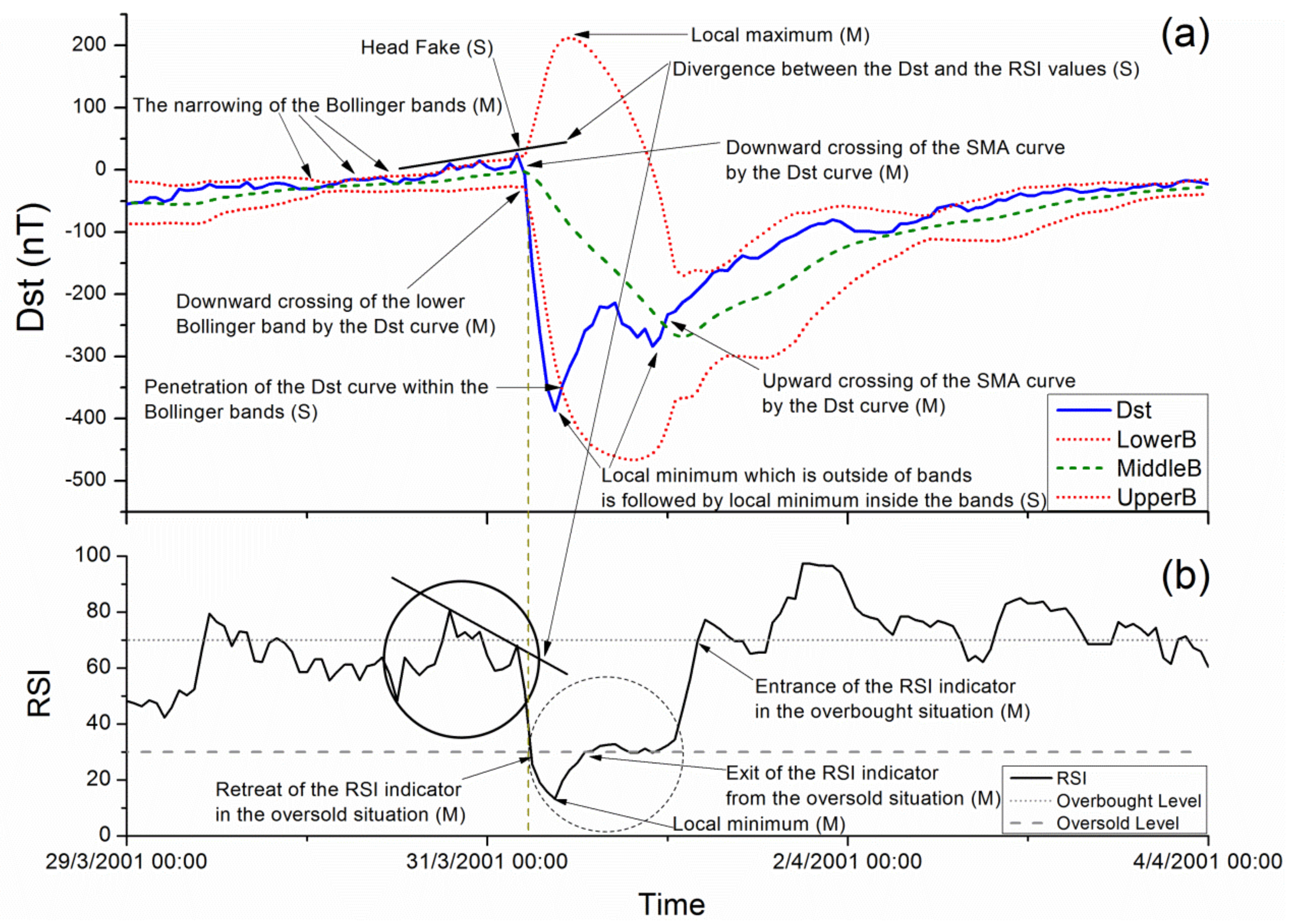
In the following, we present an analysis approach based on the time series features that can be found during the evolution, namely the onset, main development, and recovery phase, of an MS by assessing the behavior of the three considered technical analysis tools. We point out that similar features are presented on a daily basis in the financial markets in a variety of financial assets. We employ all signs, main and secondary, focusing on the temporal sequence in which they occur. The analysis approach is presented in the form of three consecutive phases, each one consisting of a set of features organized in steps according to their order of occurrence. An illustrative example of application is given in parallel using a super-storm which occurred on 31/3/2001 with a peak
value of −387 nT (see
Figure 1a, as well as line no. 13 of
Table 1).
Phase I: Preparation
(I.a) The first main feature that is presented before a possible upcoming MS is the narrowing of the Bollinger bands (M.i) (cf.
Figure 1a). The narrowing of bands indicates very low volatility of the
values preceding a volatility breakout [
73] and a corresponding extension of the bands. Immediately after the narrowing of the Bollinger bands, we assume that this will be followed by a higher volatility of
values compared to that observed during the previous period.
(I.b) In the majority of the analyzed
time series cases, it has been observed that after the narrowing of the bands and before the start of the downward movement of
, which may evolve to an MS, some secondary features are found. Although such features should only be considered as supportive of the main ones, we consider these important to mention for completeness purposes. One of them is a local maximum of
curve which exceeds the upper Bollinger band. This local maximum, often referred to as “head fake” (S.i) (cf.
Section 2.1.2), is a feature implying that the trend of the
curve in the coming hours will be downwards (see
Figure 1a). In addition, quite often, just before the beginning of the downward movement of the
curve, a “divergence” (S.ii) between the
values and the
values appears (cf.
Section 2.1.3, see
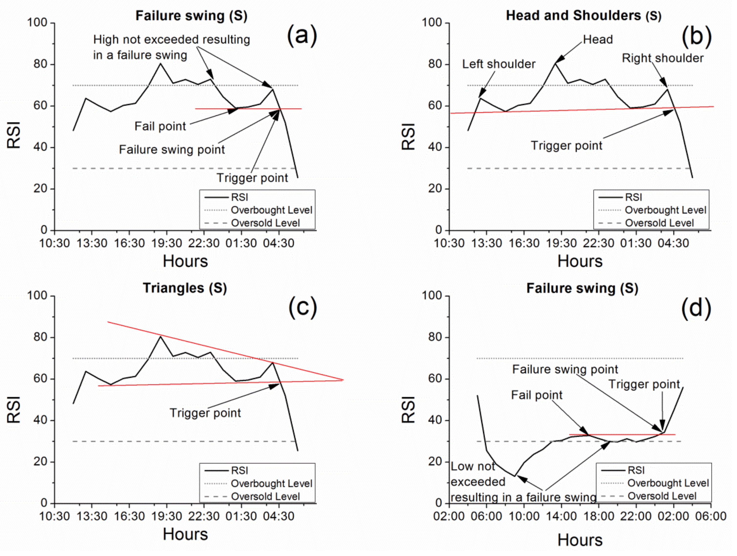
Figure 1a,b), as well as a “failure swing” (S.iii) is observed (cf.
Section 2.1.3, see solid cycle area in
Figure 1b, and enlarged in
Figure 2a), which are also features indicating a continuing downward trend of the
curve. Finally, during the same period, there have been observed, more rarely than the previous features, formulations in the
indicator known as “head and shoulders” or “triangles” (S.iv) (cf.
Section 2.1.3, see solid cycle area in
Figure 1b and enlarged in
Figure 2b,c, respectively).
Phase II: Main
(II.a) The second main feature of a possible approaching MS is a downward crossing of
curve by the
curve (M.ii), which is presented in the beginning of a downward trend of
, as shown in
Figure 1a. This is considered a very important feature, since it has been clearly identified before each one of the studied MSs. The downward movement of
usually starts a few hours earlier (cf.
Figure 1a) because, as we already mentioned, the
provides signs of trend change with a lag. Another main feature is the steep downward slope of the
indicator (M.iii) (
Figure 1b). This is indicating that
curve is moving with high speed downwards, and consequently, the MS is in full deployment. The next very important feature, of the features sequence corresponding to the main phase of an MS, is the downwards crossing of the lower Bollinger band by the
curve (M.iv) (cf.
Figure 1a, the moment of crossing is denoted by the vertical dashed line). This usually happens shortly after the downwards crossing of
; however, sometimes these two features occur simultaneously. The downwards crossing of the lower Bollinger band by the
curve is considered a main feature, since it has been identified in all the analyzed MS cases.
(II.b) In the majority of them, the
curve, after crossing the lower Bollinger band, continues to move outside the bands during the entire time period of its downward movement (S.v). This behavior, according to technical analysis literature, is a very strong indication for the evolution of the phenomenon, since it implies a continuation of the current (downward in our case) trend [
70]. However, since this is not always observed for MSs, it has been classified as a secondary feature. Note that in the differentiating cases after the downwards crossing of the lower Bollinger band by the
curve, the
curve continues moving for a while outside the bands but soon after it penetrates into the bands; however, it continues its downward movement very close, almost in parallel, to the lower Bollinger band.
(II.c) Another main feature of the deployment of the phenomenon during its main phase is the retreat of the
indicator in the oversold area (below 30) (M.v, see
Figure 1b). Note that this has, several times, been observed to occur simultaneously to the downward crossing of the lower Bollinger band by the
curve mentioned in step (II.a) (observe the vertical dashed line in
Figure 1a,b). During the same time period, we observe the downward slope of the
(M.vi); it has been observed that the steeper the slope is, the more intensive the storm is.
(II.d) The feature, which usually provides a rough, qualitative indication about the duration of the downward movement of the
curve, and, correspondingly, the duration of the MS, is the moment when the
indicator declines in the oversold situation with respect with the moment of the downward crossing of the lower Bollinger band by the
curve (S.vi) (observe the vertical dashed line in
Figure 1a,b). Specifically, as it is mentioned in technical analysis literature, “when price touches the lower Bollinger band, and
is above 30, it is an indication that the trend should continue, if price touches the lower Bollinger band and
is below 30 (possibly approaching 20), the trend may reverse itself and move upward” [
67]. This means that if we observe a simultaneous crossing (of the lower Bollinger band by the
curve and the 30 line by the
), the MS is expected to have a longer duration, while if the
drops below 30 after the crossing of the lower Bollinger band by the
curve, the storm is expected to have shorter duration. Since the expected duration of the downward movement of the
curve according to this criterion cannot be quantitatively estimated, while also in a small number of cases even a rough qualitative assessment was not possible (i.e., MSs expected, according to the specific criterion, to last long were of short duration and vice versa), the corresponding feature was classified as a secondary one. In the case presented in
Figure 1, the
drops below 30 almost simultaneously to the downward crossing of the lower Bollinger band by the
curve, which indicates that the downwards movement of the
will not last long. In this specific case, the downwards movement of the
lasted for 3 h.
Phase III: Recovery
(III.a) The first main feature which is associated with the end of the phenomenon is the curve reaching a zero slope in the oversold area (M.vii). In some cases, this feature might be found earlier than the time the curve reaches its local minimum value. However, in most analyzed cases it has been observed that the curve reaches zero slope in the oversold area concurrently with the minimum value of the curve. If the curve, after crossing the lower Bollinger band, was continuously moving outside the bands during the entire time period of its downward movement, then the re-entrance of the curve back into the bands can be taken into consideration as a secondary feature of the end of the storm (S.vii). This, along with a local minimum reached by the curve, indicates an upcoming upward move of .
(III.b) The following main feature is the curve moving away from the lower Bollinger band while a gradual reduction in the width of Bollinger bands is observed, as well as a local maximum of the upper Bollinger band (M.viii), indicating a gradual reduction of the volatility of values. At the same time, the curve is moving towards the curve (M.ix), indicating the attenuation of the phenomenon.
(III.c) Next, the exit of the
indicator from the oversold situation (M.x) is a feature associated with the upcoming ending of the phenomenon. Then, the upward crossing of the
curve by the
curve (M.xi) and the subsequent upward slope of the
curve (M.xii) are main features of the end of the MS. During the same time period, two secondary features may be observed. The first of them, which might precede the exit of the
indicator from the oversold situation, is the occurrence of two local minima of the
curve, one outside the Bollinger bands, followed by a second inside the bands forming a W-shaped curve (S.viii). The other secondary feature, which always follows the exit of the
indicator from the oversold situation, is a failure swing in the
curve, implying also the upward trend of
(S.iii) (cf.
Section 2.1.3, see dashed cycle area in
Figure 1b, and enlarged in
Figure 2d).
(III.d) The final feature found during the termination of the phenomenon is the entrance of the indicator to the overbought situation (M.xiii), which implies that the upward trend of the curve is strong before it returns to the quiet conditions.
In summary, each one of the abovementioned phases presents at least the following features, in the specific sequence per phase and step (indicating also the corresponding notation for numbering phases, phase steps, and main and secondary features):
Phase I:
Phase II:
Step (II.a): Downward crossing of the curve by the curve (M.ii).
Step (II.a): Steep downward slope of the indicator (M.iii).
Step (II.a) Downward crossing of the lower Bollinger band by the curve (M.iv).
Step (II.c): Retreat of the indicator in the oversold area (below 30) (M.v).
Step (II.c): Steep downward slope of the curve (M.vi).
Phase III:
Step (III.a): Zero slope of the curve in the oversold area (M.vii).
Step (III.b): The curve moving away from the lower Bollinger band and the start of a gradual reduction in the width of Bollinger bands, as well as a local maximum at the upper Bollinger band (M.viii).
Step (III.b): The curve moving towards the curve (M.ix).
Step (III.c): Exit of the indicator from the oversold situation (M.x).
Step (III.c): Upward crossing of the curve by the curve (M.xi).
Step (III.c): Upward slope of the curve (M.xii).
Step (III.d): Entrance of the indicator to the overbought situation (M.xiii).
It is highlighted that all of these features have been found to occur for all the examined cases of MSs.
4. Analysis Results
The applicability of the analysis approach proposed in
Section 3 for the analysis of the
time series during MSs based on stock market (technical analysis) tools is examined in detail on four characteristic cases of MSs. Moreover,
Table 1 shows which of the considered features (per phase and step) were identified for each one of the 24 analyzed MSs. The corresponding informative plots, which summarize the analyses results for each one of the MSs listed in
Table 1, are also provided as online
supplementary material.
4.1. First Case Study
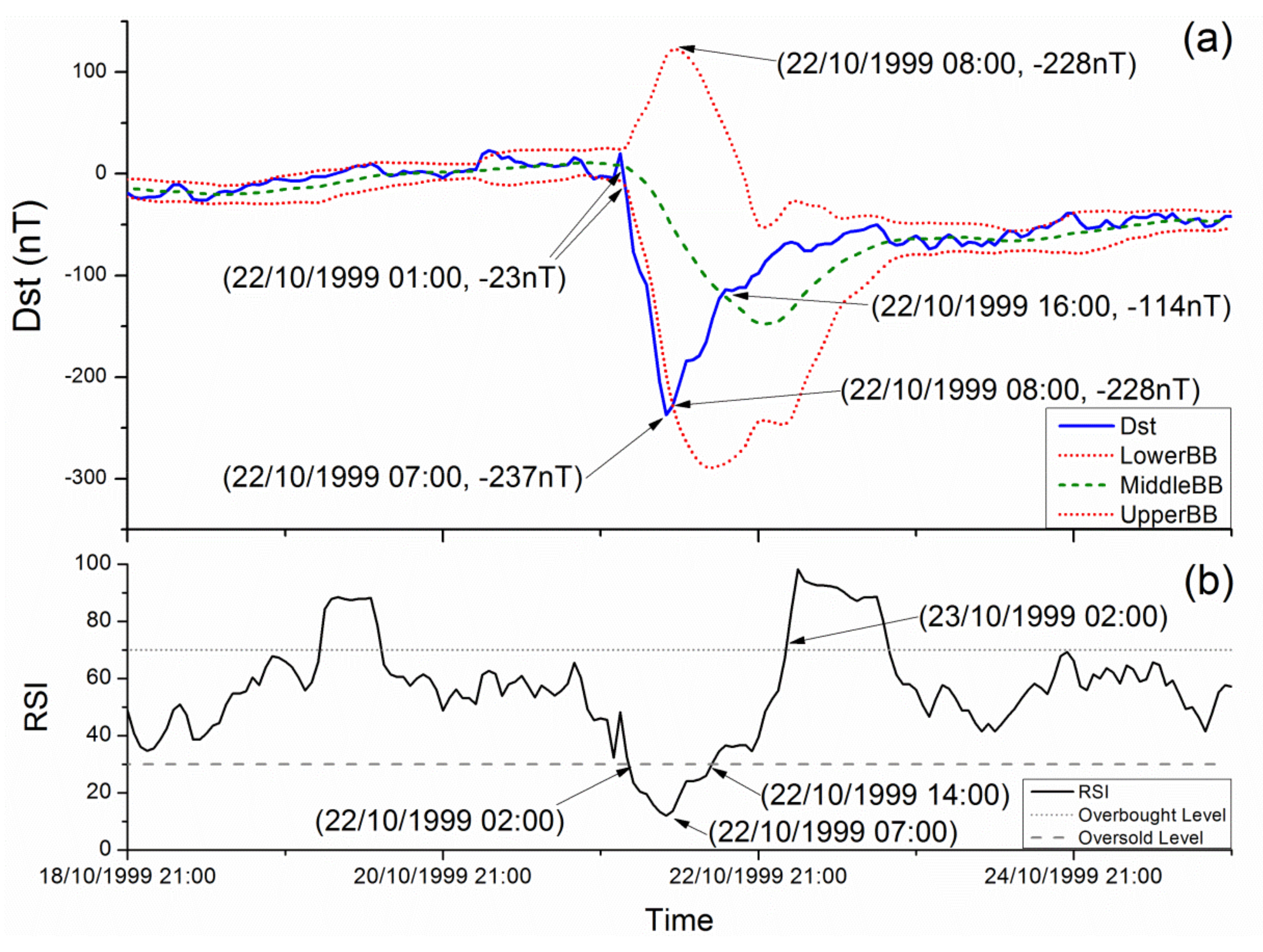
The first case we examine is that of the storm that occurred on 22 October 1999 (see line no. 10 of
Table 1); the analyses results are portrayed in
Figure 3. The evolution of the specific MS in terms of the phases and corresponding steps described in
Section 3 follows:
Phase I: Preparation
In
Figure 3, we observe a (prolonged) narrowing of Bollinger bands, from 18 October 1999 21:00 until 22 October 1999 01:00. As already mentioned in step (I.a) of
Section 3, this is a first feature for a possible upcoming MS. Note that the secondary features described in step (I.b) are not observed in the specific case.
Phase II: Main
Step (II.a): A few hours later, on 22 October 1999 01:00, we can see that two main features appear simultaneously, namely the downward crossing of the curve and the lower Bollinger band by the curve. At this point, we should mention that the indicator is also moving with a steep downward slope towards the oversold (under 30) area, indicating that the values move with high speed downwards.
Step (II.b): As long as the curve moves downward outside the Bollinger bands, a continuation of the current (downward) trend is implied.
Step (II.c): One hour later, on 22 October 1999 02:00, the indicator retreats below 30, while the value is −77 nT. During the next five hours, the downward movement of continues, while in parallel, the curve retreats with steep slope, concluding the sequence of main features related to the deployment of the MS.
Step (II.d): At this point, we should note that at the moment when the
curve downward crossed the lower Bollinger, the
indicator had not yet reached its lower threshold value of 30. This, as it has been observed in the majority of the examined MS cases (cf.,
Section 3), means that the downward movement of the
, and consequently the MS, is expected, as a rough qualitative assessment, to last for a long time, provided that the
indicator finally retreats below 30, as it indeed happens in our case.
Phase III: Recovery
Step (III.a): On 22 October 1999 07:00, concurrently with the minimum value of the curve, the curve has almost zero slope verifying the reversing of the downward trend of the curve.
Step (III.b): On 22 October 1999 08:00, while the curve starts the upward movement, it enters again into the Bollinger bands, while at the same time the upper Bollinger band presents a local maximum, enhancing the features associated with the definite completion of the downward movement of the curve. Subsequently, we observe that the curve, as it moves upwards, moves towards the curve, while at the same time moves away from the lower Bollinger band. Note that, in parallel, the width of Bollinger bands is gradually reduced, indicating a gradual reduction of the volatility of values.
Step (III.c): After that, we identify two more main features related with the ending of the phenomenon: first, the
indicator exits the oversold situation on 22 October 1999 14:00, while two hours later, the upward crossing of the
curve by the
curve happens. Note that the secondary features of step (III.c) described in
Section 3 were not observed in the specific MS case.
Step (III.d): Finally, on 23 October 1999 02:00, the indicator enters the overbought situation, signifying the conclusion of the MS.
4.2. Second Case Study
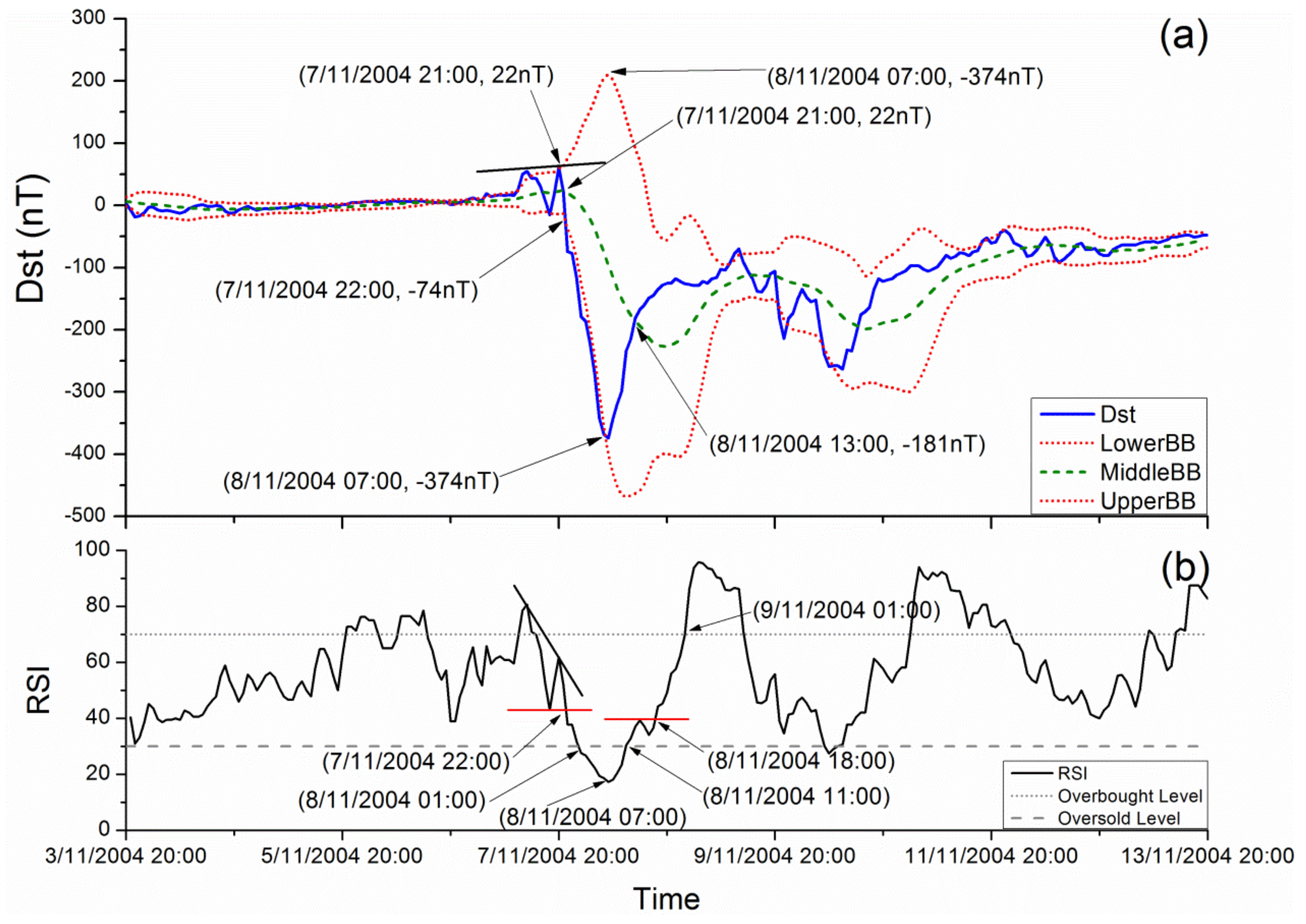
Next, we examine a storm which occurred on 8 November 2004 (see line no. 18 of
Table 1), while the corresponding analyses are shown in
Figure 4.
Phase I: Preparation
Step (I.a): First, we observe that there is a (prolonged) narrowing of the Bollinger bands from 3 November 2004 20:00 until 06 November 2004 19:00.
Step (I.b): At 21:00 of the next day, we can see two secondary features of the preparation phase, namely the head fake and the divergence between the curve and the indicator. Moreover, in parallel, the indicator curve forms a failure swing. Although these are secondary features, they enhance the evidence in favor of an upcoming MS, since they imply a continuing downward movement of .
Phase II: Main
Step (II.a): Right after this, the downward crossing of the curve by the curve is observed, while one hour later the downward movement of the curve continues and crosses the lower Bollinger band. Moreover, the indicator is moving with a steep downward slope towards the oversold (under 30) area, indicating that the values move with high speed downwards.
Step (II.b): At this point, we observe that the curve moves downward outside the Bollinger bands. As long as this is satisfied, a continuation of the current (downward) trend is implied.
Step (II.c): On 08 November 2004 01:00, the indicator curve retreats below 30. During the next six hours, the downward movement of continues, while in parallel, the curve retreats with steep slope.
Step (II.d): At this point we should take into account that the indicator reached the low threshold value of 30 later than the moment when the curve crossed downwards the lower Bollinger. In other words, the indicator had a value higher than 30 when the curve crossed downwards the lower Bollinger, indicating, as a rough qualitative assessment, that the downward movement of the is expected to last for a long time.
Phase III: Recovery
Step (III.a): On 08 November 2004 07:00, we observe three features associated with the upcoming change of the curve move to an upwards one; namely, the curve slope almost reaches zero, while at the same time, the curve reaches its local minimum value and penetrates into the Bollinger bands.
Step (III.b) At the same time, a local maximum is observed in the upper Bollinger band, indicating that the downwards trend of the curve will soon be changed to an upwards one. Indeed, one hour later the curve trend changes to upwards. From this point on, the curve moves upwards approaching the curve, departing from the lower Bollinger band, while the bands gradually narrow.
Step (III.c): Then, the indicator gradually moves upwards, leading to a feature found near the ending of the MS: the exit of the indicator from the oversold situation which occurs on 8 November 2004 11:00. Following that, the next main feature is the upward crossing of the curve by the curve, which takes place on 8 November 2004 13:00. From this point on, although with a certain delay, the curve develops an upwards slope. Five hours later, on 8 November 2004 18:00, a secondary feature, a failure swing, appears in the indicator curve, enhancing the evidence in favor of the upward trend of the curve.
Step (III.d): Finally, the upcoming definite conclusion of the MS is signified by the entrance of the indicator into the overbought situation on 9 November 2004 01:00.
It is finally noted that for the specific time period presented in
Figure 4, one can observe that ~2 days after the above-analyzed MS, and while
has not yet reached quiet levels, a second weaker MS, but still an intense event (minimum
value~−250 nT), took place. While one could identify some of the technical analysis features (presented in
Section 3) which, according to the proposed analysis approach, are found during the evolution of an MS, it is not possible to identify the complete sequence of main features. Therefore, we have to mention that in this case, the proposed analysis approach is not able to discriminate between the two sequentially appearing MSs.
4.3. Third Case Study
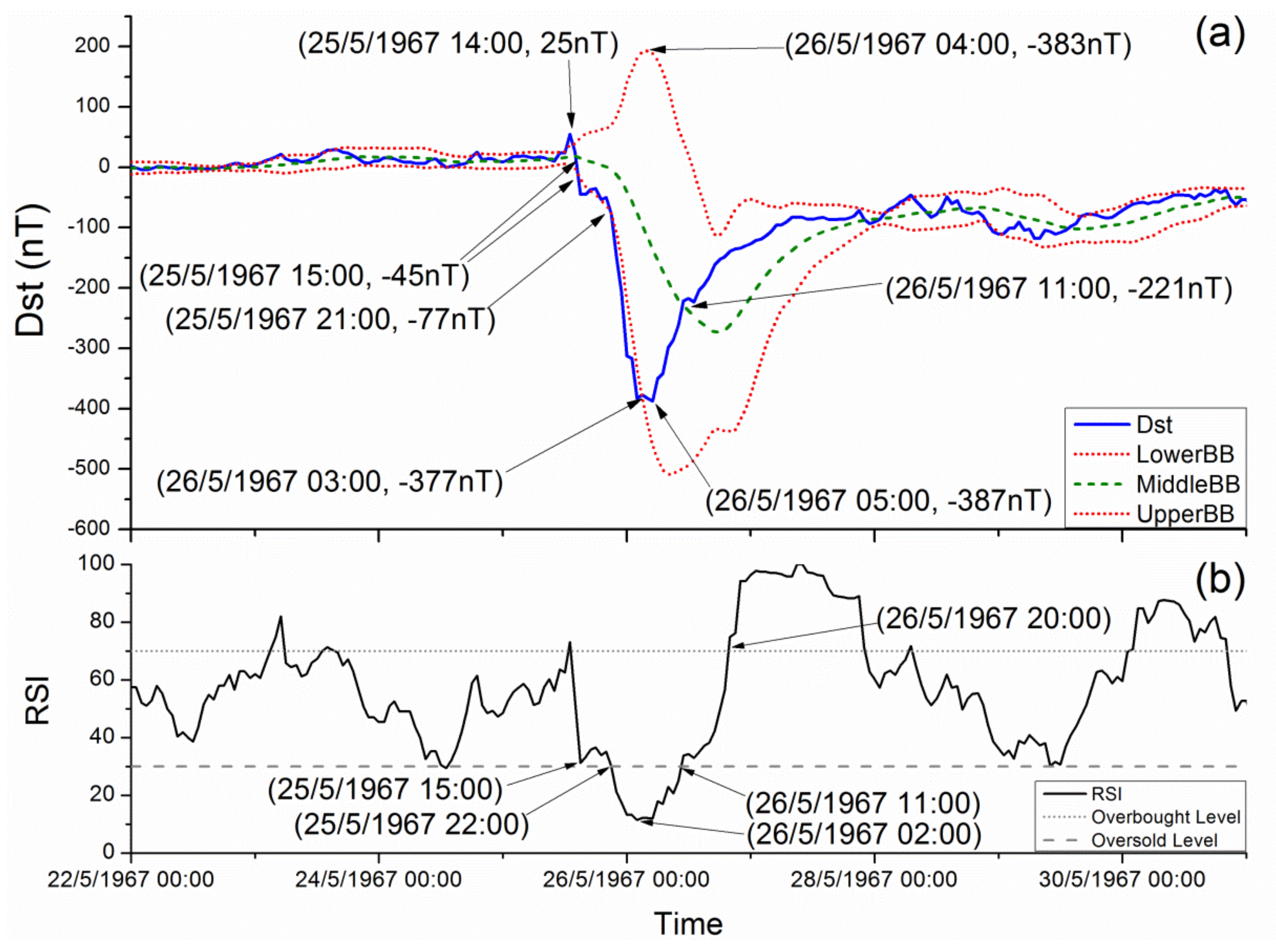
The third MS analyzed in terms of technical analysis tools is a storm which occurred on 26 May 1967 (see line no. 8 of
Table 1), while the corresponding analyses are shown in
Figure 5. For the specific MS, we can identify the following sequence of features associated with its evolution by short-term analysis.
Phase I: Preparation
Step (I.a): From 22 May 1967 00:00 up to 25 May 1967 12:00, we observe a prolonged narrowing of the Bollinger bands, the first main feature of an upcoming MS.
Step (I.b): On 25 May 1967 14:00, we observe that a head fake is formed over the upper Bollinger band, which is a secondary feature indicating an upcoming downward trend of the curve. Note that this is the only secondary feature that was identified at this step for the specific storm.
Phase II: Main
Step (II.a): The expected downward trend of the
curve indeed happened one hour later, on 25 May 1967 15:00, when the
curve simultaneously crossed downwards both the
curve and the lower Bollinger band. Both these crossings are main features of the beginning of an MS. Turning now to the
indicator, we can see that although it was moving with a steep downward slope towards the oversold situation, indicating a high downward speed for
values, it finds support at the 30 level. During the next five hours, the
curve moves inside the Bollinger bands, close to the lower band. However, the width of the bands continues to expand. On 25 May 1967 21:00 we observe that the
curve crosses once more the lower Bollinger band downwards. Note that between these two downward crossings of the lower Bollinger band, the
curve moves inside the bands, i.e., step (II.b) has not yet been observed. As already mentioned in
Section 3, this step corresponds to a secondary feature which is not always observed after a downwards crossing of the lower Bollinger band by the
curve, so we do not pay any special attention to this fact. After the second crossing of the lower Bollinger band, we also notice that the
indicator moves with a steep downward slope, which is gradually reducing.
Step (II.b): From 25 May 1967 21:00 onwards, the curve remains outside the Bollinger bands, indicating a continuation of its current (downwards) trend.
Step (II.c): The indicator again moves downwards to the oversold situation to retreat below the 30 level one hour later. At the same time, we note that the curve gradually begins to move downwards with steep slope, indicating a strong downwards trend for .
Step (II.d): Given that the curve downward crossed the lower Bollinger band before the indicator retreated below 30, we expect, as a rough qualitative assessment, that the downward movement of until it reaches its lowest value will last for a long time (in the specific case, this lasted for 6 h).
Phase III: Recovery
Step (III.a): On 26 May 1967 02:00, the curve reaches almost zero slope, indicating that the downward trend of the curve is soon expected to be reversed to an upward trend. One hour later, at 03:00, we can see that the curve penetrates inside the Bollinger bands, which is a secondary feature enhancing the possibility that the trend is soon expected to be upward.
Step (III.b): One hour later, on 25 May 1967 04:00, a local maximum of the upper Bollinger band is observed, which is a main feature also informing us about the upcoming upwards trend of the curve. Next, the curve moves towards the curve and away from the lower Bollinger band, while, in parallel, the width of the bands is gradually reducing.
Step (III.c): On 26 May 1967 11:00, two main features appear, simultaneously related to the ending of the phenomenon. Specifically, the curve upward crosses the curve, and, soon after, the develops an upwards slope, while the indicator exits the oversold situation.
Step (III.d): Finally, on 26 May 1967 20:00, we observe the indicator entering the overbought situation, which signifies the definite completion of the phenomenon.
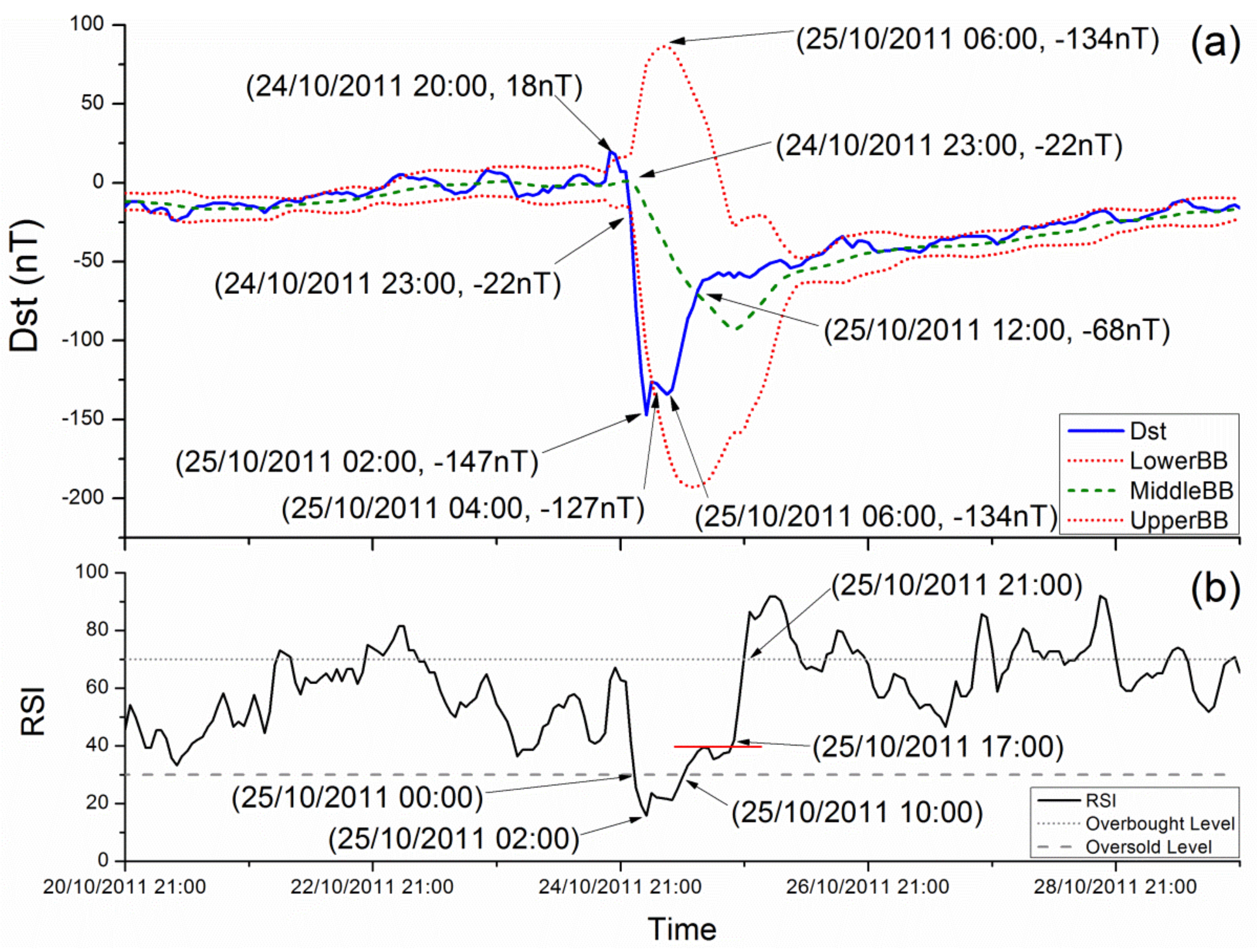
4.4. Fourth Case Study
The last MS case is an intense storm which occurred on 25 October 2011 (see line no. 23 of
Table 1); the corresponding analyses are shown in
Figure 6. The evolution of the specific MS in terms of the phases and corresponding steps described in
Section 3 follows:
Phase I: Preparation
Step (I.a): From 20 October 2011 21:00 up to 24 October 2011 19:00, we observe a prolonged narrowing of the Bollinger bands, which, as already mentioned in
Section 3, is a main feature observed before an upcoming MS.
Step (I.b): On 24 October 2011 20:00, although, until then, the
curve was moving mainly within Bollinger bands, we observe a head fake which is expected before an upcoming downtrend in the
curve. Other secondary features, of the ones corresponding to the specific step in
Section 3, were not observed for the specific MS.
Phase II: Main
Step (II.a): A few hours later, on 24 October 2011 23:00, we can see that two main features appear simultaneously, namely the downward crossing of the curve and the lower Bollinger band by the curve. We also observe that the indicator is moving with a steep downward slope towards the oversold (under 30) area, indicating that the values move with high speed downwards.
Step (II.b): After the crossing of the lower Bollinger band by the curve, the curve moves downward outside the Bollinger bands, signifying a continuation of the current (downward) trend.
Step (II.c): On 24 October 2011 00:00, the indicator enters the oversold situation, while, from this point on, the curve moves downwards with a steep slope.
Step (II.d): This specific MS is an example for which step (II.d) does not provide a correct assessment for the duration of the MS. Although the retreat of the indicator into the oversold situation was delayed with respect to the moment when the downward crossing of the lower Bollinger band by the curve occurred, the duration of the downward movement of the curve, and correspondingly the duration of the MS, was not long. Remember that the specific feature was classified as a secondary one, exactly due to the reason that there are MS cases, even though they are very few, for which it does not provide even a rough qualitative assessment for their expected duration, in addition to the fact that it is not possible to provide a quantitative assessment for the expected duration, only a rough qualitative assessment.
Phase III: Recovery
Step (III.a): On 25 October 2011 02:00, we observe that the indicator almost reaches zero slope, indicating that the curve will possibly move upwards during the following hours. The curve also reaches its local minimum value then, while, two hours later, the curve enters back into the Bollinger bands, one more feature observed when the phenomenon is led to its completion.
Step (III.b): Following that, on 25 October 2011 06:00, we observe a local maximum of the upper Bollinger band, suggesting the upcoming reduction of values’ volatility, as well as a secondary feature, usually observed later, and for this reason described as part of step (III.c), the occurrence of two local minima of the curve, one outside the Bollinger bands followed by a second inside the bands forming a W-shaped curve. During the next hours, the curve develops an upwards slope towards the curve, while at the same time, the width of the Bollinger bands is gradually reduced and the curve moves away from the lower Bollinger band, all implying a return to normal (quiet) values.
Step (III.c) On 25 October 2011 10:00, the curve exits the oversold situation, while two hours later, the curve upward crosses the curve, which then moves with an upwards slope, complementing the features related to the ending of the phenomenon. Moreover, on 25 October 2011 17:00, a failure swing is observed, which is a secondary feature.
Step (III.d): The final recovery phase feature, signifying the conclusion of the MS, occurs on 25 October 2011 21:00, when the indicator enters the overbought situation.
5. Discussion—Conclusions
In the frame of complex systems, we studied the time series of in terms of the empirical financial analysis method known as technical analysis, focusing on the temporal evolution of MSs. Specifically, we employed the combination of three very popular tools of technical analysis, the simple moving average (), the Bollinger bands, and the relative strength index (). The goal of this exploratory study was to formulate an analysis approach of time series during the evolution of MSs in analogy to asset price time series analysis in high volatility periods.
This analysis approach was developed after the analysis of more than 20 MS events, revealing all the technical analysis features (appearing in financial time series during high volatility periods, e.g., [
67,
73]) which, in specific temporal sequence of occurrence, appear associated with the onset, main development, and recovery phase of an MS. It is emphasized that, in the proposed analysis approach, the feature sequence is important in the evolution of an MS, and not merely each feature by itself. For example, a downward crossing of the
curve by the
curve, per se, without the preceding and following main features, does not imply a new MS. The applicability of the proposed analysis approach was presented in detail for four characteristic cases of MSs, while the results for the whole set of 24 analyzed MSs verify the repeatability of the proposed features’ sequences.
We focus on the fact that the results of this study enhance the view that quantitative analysis methods may successfully be transferred between finance and geophysical systems. Our results show that time series around the occurrence of MSs can be successfully analyzed by the same empirical tools applied to financial time series for investment analysis.
In general, when a new MS is developing, the sequence of features described by the proposed analysis approach is repeated. However, clearly, the presented analysis approach is not suggested as a method for the early detection of MSs. The main shortcomings for such an application are mentioned in the following. Magnetic storms are not always preceded by quiet conditions and, in such cases, the narrowing of the Bollinger bands feature before an MS may not be clearly identified or even not identified at all, while on the other hand, a narrowing of the Bollinger bands may be observed in quiet conditions without an MS to follow, and it is not possible to predict whether double or multiple storms will occur. Moreover, it is not possible to predict what the minimum value of
will be, or whether the minimum
value will exceed some specific threshold, e.g., −50 nT, −100 nT, etc.; only the short-term trend is inferred. As a result, the described sequence of features may be observed even in the case of variations that do not exceed −50 nT. Additionally, it is not possible to predict when the
minimum will occur or to provide a quantitative assessment for the duration of an MS. Characteristic examples highlighting these shortcomings are the following: the MSs no. 20–21 of
Table 1 (see also online
supplementary material) where the two MSs that happened with ~8 days distance and had minimum
values −184 nT and −122 nT, respectively, presented the same main features of the
time series. The variation of the
~2 days before the MS no. 17 of
Table 1 (see also online
supplementary material), despite the fact that it reaches a minimum value of only ~ −30 nT, presents most of the main features observed in all the analyzed MSs. The
time series of the second case study (
Figure 4) presents a second minimum of the order of −200 nT, around which the considered features are not all clearly found.
These shortcomings call for further investigation of the proposed use of the considered technical analysis tools in the study of MSs. This should primarily focus on the tuning of analysis parameters based on extensive statistics resulting from the application of the specific tools for long enough time periods, e.g., for the last two solar cycles. Note that the considered technical analysis methods were applied to time series directly adopting mutatis mutandis in terms of sampling rate scale, the parameter values usually employed for the analyses of financial time series. Specifically, the usually employed parameter values for the calculation of and Bollinger bands when applied to daily stock market share data were also used for the case of hourly data.
Moreover, after an appropriate tuning of the proposed analysis’ parameters, we consider the worth of investigating its combination with other statistical and complex systems time series analysis methods, such as different kind of entropies, Hurst exponent, fractal analysis, and log-periodic corrections. Furthermore, by incorporating solar wind data in the proposed combined multi-method analysis scheme, we may improve the diagnostics of the coupled solar wind–magnetosphere system and, consequently, the mitigation of space weather hazards. Although this is outside the scope of this specific work, it is in our near future plans to elaborate such a study.
As already clarified, the here-presented study followed the empirical way of analyzing financial time series for the analysis of time series, trying to identify features also used in financial time series, which could be associated with the temporal evolution of an MS. In a next step, one could focus on the interpretation of the observed behavior of the considered financial tools, in terms of the physics of the magnetosphere. Such a study could, on one hand, increase the effectiveness of the proposed analysis approach for the study of MSs, and, on the other hand, offer ideas in order to better understand stock market processes.
It has been established that natural hazards may result in geospace perturbations. For instance, it has been suggested that ionospheric perturbations could be attributed to earthquake events [
85,
86,
87,
88]. The promising results from the application of financial analysis tools to geomagnetic activity index time series, regarding the study of geomagnetic perturbations related to an MS, may also offer a useful framework of technical analysis for the study of geospace perturbations related to other natural hazards (e.g., earthquakes, tsunamis etc.).


